Machine Learning Altitude Estimation from Smartphone Accelerometer Elevator Data

Abstract

While Global Positioning System (GPS) devices attain horizontal accuracy within a few meters, they fail vertically indoors with inaccuracies more than 10 meters. Heating, ventilation, and air conditioning (HVAC) systems and climatic variations make barometric pressure sensors, which are frequently employed as an alternative, inaccurate. In real-world situations, typical inaccuracies can reach 3–5 meters (about 1.0–1.5 stories). In order to eliminate the requirement for barometric sensors or external infrastructure, this work proposes a unique machine learning-based method for floor-level estimation utilizing only smartphone accelerometer data during elevator traversals. We gathered fifty elevator rides from five distinct elevators in commercial office buildings. These rides included both uphill and descending journeys, with each traversal lasting one to ten stories. Two different approaches were compared: (1) a lightweight 1D Convolutional Neural Network that operates directly on raw acceleration time series, and (2) a feature-based Random Forest regressor that uses seven physics-informed features extracted from acceleration signatures (duration, peak acceleration, mean energy, and integrated velocity extrema). The feature-based technique, with a Mean Absolute Error of 0.48 floors (~1.6m assuming 3.3m per floor, R² = 0.96) on the test set, outperformed the deep learning model (MAE = 2.78 floors, ~9.2m R² = −0.06) in this pilot study, which showed instability because of the limited dataset size. These preliminary findings suggest that in small-data regimes, physics-informed feature engineering may outperform end-to-end deep learning, allowing for promising vertical positioning without barometric sensors. By offering preliminary evidence for a hardware-independent approach tested under controlled single-user conditions in 5 commercial office elevators, this pilot study contributes toward smartphone-based indoor localization.

Keywords: GPS vertical accuracy, machine learning, elevator vibration recognition, smartphone accelerometer, feature engineering, floor-level detection, small-data machine learning, indoor positioning

Introduction

Background and Context

In multistory buildings, indoor vertical localization has grown in significance for navigation, asset management, and emergency response. Global Positioning System (GPS) technology is quite good at horizontal location, with accuracy within a few meters in open spaces. However, indoor signal attenuation causes vertical errors that are more than ten meters^1,2.

Modern smartphones incorporate barometric pressure sensors to measure altitude in order to overcome this constraint. However, localized pressure changes from HVAC systems, elevator shafts, and building pressurization cause barometer methods to deteriorate considerably indoors^3,4,5.

Even under ideal conditions, research shows that smartphone barometers have vertical inaccuracies of 3–5 meters, or around 1.0–1.5 stories⁶. This is insufficient to differentiate between adjacent floors, which are normally only 3–4 meters apart⁷.

Problem Statement and Rationale

Without extra gear or infrastructure, current GPS and barometer-based techniques are unable to accurately identify particular floor levels. As a result, a technique that determines floor levels without the use of ambient measures and solely using common smartphone sensors is desperately needed^8,9,10.

Almost every smartphone has an accelerometer, which records the natural dynamics of elevator motion: acceleration at commencement, a comparatively constant speed when moving, and deceleration while stopping. These motion signatures show promise for reliable floor-level estimation as they are not subject to the pressure variations that affect barometric sensors¹¹.

Significance and Purpose

An infrastructure-free, barometer-independent approach for accurate floor-level estimate utilizing smartphone accelerometer data is presented in this study. We provide preliminary evidence that vertical positioning may be accomplished without pressure sensors or GPS by using machine learning to acceleration signatures, with potential applicability across smartphone models and building types subject to further validation.

This pilot study contributes to the growing body of work on smartphone-based indoor positioning, which also explores potential solutions for location-aware services, package delivery routing, and emergency response^12,13,14,15.

Objectives

The primary objectives are to:

Scope and Limitations

The accelerometer data from smartphones taken during elevator rides in business office buildings is the main subject of this investigation. The dataset includes 50 traversals over floor distances ranging from 1 to 10 stories in five different elevators. Limitations include:

Theoretical Framework

The study is based on machine learning and signal processing influenced by physics. The kinematic pattern of elevator motion is clearly defined: acceleration a(t) → velocity v(t) = ∫ a(t) dt → displacement z(t) = ∫ v(t) dt. We construct a feature space that encapsulates the essential connection between motion dynamics and vertical displacement by extracting characteristics that correspond with this physical process. The nonlinear link between these physics-informed features and actual floor difference is then learned by a Random Forest regressor. This allows the model to capture variability across different elevators and operating conditions¹⁶.

Methodology Overview

The floor estimating system was developed and assessed in this work using a four-phase experimental methodology. First, the phyphox smartphone sensor recording program (version 1.2.0) was used to gather accelerometer data from fifty controlled elevator rides. Second, in order to separate pure elevator motion, raw acceleration signals were preprocessed (noise filtering, spike removal, active segment recognition). Third, two different models were created. The first was a 1D CNN operating on raw time-series data; the second was a feature-based Random Forest using seven physics-informed features. The Google Colab cloud computing infrastructure with Python-based machine learning packages was used for both model training and evaluation. Lastly, a held-out test set was used to evaluate performance by comparison analysis; the detailed findings are shown in the sections that follow.

Overall Modeling Pipeline

Figure 1 summarizes the end-to-end modeling workflow used in this study. In order to get noise-filtered segments segmented by a minimum motion duration of 1.0 s, raw Z-axis accelerometer signals with timestamps were first gathered during elevator traversals and then run through the preprocessing pipeline outlined in Section 2.3.

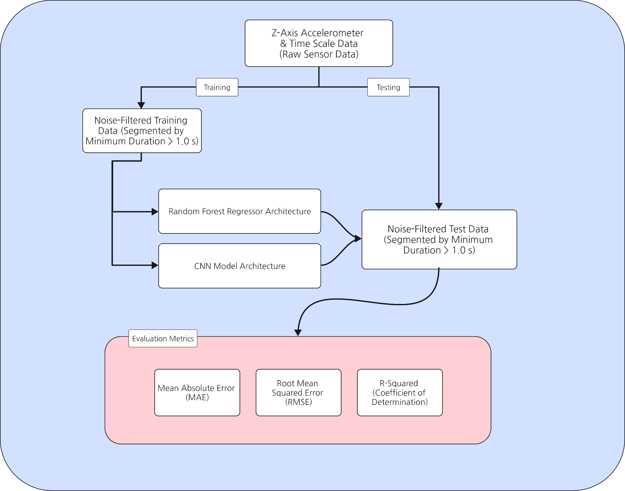
The left branch of the framework represents the feature-based approach, in which noise-filtered training segments are transformed into a seven-dimensional feature vector and used to train a Random Forest regressor. The right branch represents the end-to-end deep learning approach, where the same trimmed segments are zero-padded and fed directly into a 1D CNN architecture.

The regression metrics used to compare the two models on the test set are highlighted in the bottom evaluation block: R² to measure the percentage of variance in floor difference explained by each model, RMSE to penalize big errors, and MAE for average floor-level error.

Methods

Research Design

In order to assess two different methods—feature-based machine learning and end-to-end deep learning—this study used a controlled experimental design with a comparison framework. The investigation comprised four phases: (1) data collection from 50 elevator traversals, (2) data preprocessing and feature extraction, (3) model development, and (4) comparative performance evaluation.

Participants and Data Collection

A Single researcher (17 years old) gathered data from 50 controlled elevator rides across five commercial office buildings, covering both ascending and descending journeys over one to ten stories. Data were recorded using the phyphox mobile application (version 1.2.0) on an iPhone 14 at approximately 100 Hz¹⁷. Off-peak hours were chosen to minimise interruptions; any ride interrupted by an intermediate stop was discarded and repeated. Ground truth floor labels were read directly from building directories and elevator cabin displays, and encoded in the filename following the convention [Elevator][Start]-[End]-[Trial].xls. The full step-by-step data collection procedure is provided in Appendix A.

Data Preprocessing and Active Segment Extraction

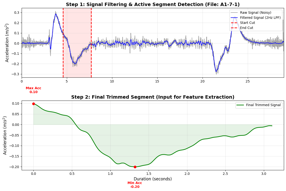
Significant amount of noise and irrelevant periods like idle time before or after arrival exist in raw acceleration data gathered from smartphones. We developed a multi-stage preprocessing pipeline to extract the Active Segment, the precise time frame that represents the elevator’s vertical displacement, in order to guarantee the machine learning model’s stability.

Figure 2 illustrates this process, visualizing the transformation from raw signals to the final trimmed segment used for training.

Signal Conditioning Pipeline

The preprocessing was implemented in Python using scipy and numpy, consisting of the following steps. All signals were recorded at approximately 100 Hz (as described in Section 2.2.2), giving a time resolution of 0.01 s per sample:

A cutoff of 2.0 Hz was selected because elevator acceleration profiles are dominated by low-frequency components: the typical acceleration and deceleration phases of a commercial elevator occur over 1–3 seconds, corresponding to a fundamental frequency well below 1 Hz. Frequencies above 2.0 Hz in the raw signal primarily represent hand tremors, footstep vibrations, and sensor noise, which are irrelevant to the vertical displacement estimation task. This cutoff is consistent with values used in prior inertial sensor-based vertical motion studies^18,10.

The elevator motion window was successfully isolated by this preprocessing, which reduced the raw data from 3,000–8,000 samples to a cleaned segment of 500–2,500 samples per traversal.

Kinematic Justification for Trimming

We only use the shortened segment for training, as seen in the bottom panel of Figure~2 (green region). This choice is based on kinematics since the summation of acceleration over this particular time period physically determines the vertical distance (floor level).

The displacement and velocity are obtained using the equations of kinematics as follows:

   

Because of this relationship, (Maximum Acceleration) and (Minimum Acceleration) are important characteristics, but they are insufficient without the temporal context ().

Physics-Informed Feature Extraction

From each trimmed acceleration signal, seven features were extracted to encode these kinematic properties:

These seven features formed a low-dimensional representation x ∈ ℝ⁷ for each traversal, with the target variable defined as: floor_diff = end_floor − start_floor

Model Development

Google Colab

a cloud-based Jupyter notebook environment that offers free GPU acceleration, was used for all model training and evaluation. Python 3.9 with the scikit-learn (version 1.2), TensorFlow/Keras (version 2.12), pandas, and matplotlib libraries were used in the implementation¹⁹. Complete code is provided in Appendix B.

Physical Feature-Based Model (Model A): Random Forest Regressor

The seven-dimensional feature vectors were used to train a Random Forest model with 100 decision trees. For reproducibility, the following hyperparameters were set: random state = 42, minimum samples per leaf = 2, and maximum tree depth = 10. Because of the limited training set (N = 40, after 80% split), these conservative hyperparameters were used to avoid overfitting. On the training set, 5-fold cross-validation was used to validate the hyperparameter selection¹⁶.

Physical Raw Sequence Model (Model B): 1D Convolutional Neural Network

A purposefully lightweight CNN architecture with L2 regularization (λ = 0.01) and Dropout layers (p = 0.3) was created in order to fairly compare with deep learning techniques while minimizing the danger of overfitting^20,21.:

This specific architecture, input length, and training configuration were selected as a single representative deep learning baseline for comparison purposes. No systematic hyperparameter search, architecture ablation, data augmentation, or alternative sequence model designs (e.g., fully connected networks operating on raw sequences, shallower single-layer CNNs, or recurrent architectures) were explored. The goal was not to find the optimal deep learning solution for this problem, but rather to establish whether a standard lightweight 1D CNN architecture — a commonly used baseline for sensor time series^22,23 — is viable on a dataset of this size. The fixed input length of 3,000 samples was chosen as a conservative upper bound slightly exceeding the observed maximum trimmed segment length of 2,500 samples, ensuring no real signal was truncated. However, for the shortest segments (~500 samples), up to 83% of the input consisted of uninformative zero-padding, which may have diluted the CNN’s learned representations and adversely affected the GlobalAveragePooling operation independently of the dataset size issue.

With batch size 8, Adam optimizer (learning rate 0.001), mean squared error (MSE) loss function, and 10% validation split from the training set, training was carried out for 100 epochs. With a total of ~200 parameters, the sparse architecture was purposefully created to avoid memorization of the limited training set. The zero-padding strategy represents a further confound in the CNN comparison, making it difficult to isolate the effect of data scarcity alone from the effect of uninformative padding. Alternative approaches such as using the 95th percentile sequence length as MAX_LEN, pre-padding, or variable-length architectures were not explored and are identified as directions for future work.

Train-Test Split and Evaluation Metrics

Stratified random sampling (random state = 42) was used to divide the 50-sample dataset into training (40 samples, 80%) and test (10 samples, 20%) sets. Stratification was performed on direction of travel (ascending vs. descending) to ensure that both ascending and descending rides were proportionally represented in both sets. It should be noted that this random split does not ensure elevator-level separation: rides from the same elevator and building may appear in both the training and test sets. As a result, the reported metrics reflect within-distribution performance across seen elevators rather than true generalization to unseen elevators or buildings. A leave-one-elevator-out (LOEO) or leave-one-building-out evaluation would be required to properly assess cross-elevator generalizability, and is identified as a priority for future work. To guarantee a reliable comparison, both models were assessed using the same test set.

Performance metrics included:

Mean Absolute Error (MAE):

   

Coefficient of Determination (R²):

   

Root Mean Squared Error (RMSE):

   

Here, yᵢ denotes the ground-truth floor difference for sample i, and ŷᵢ denotes the corresponding model-predicted floor difference.

Data Analysis

Error distribution histograms, scatter graphs comparing actual versus anticipated floor disparities, and per-elevator performance breakdowns were used to examine model predictions. MAE and R² were used as the main measures for model selection in the statistical comparison.

Ethical Considerations

Data privacy and research integrity were carefully considered during the design of this single-participant study. Sensor timestamps and building identifiers were the only individually identifiable information in the data, which was entirely under the researcher’s sole control. All data was kept locally on password-protected devices and was not transmitted to external servers. Prior to data collection, verbal permission was obtained from the facility management office of each building, who confirmed that non-commercial academic sensor recording in common areas (elevator cabins) was permitted. No personally identifiable information about other building occupants was collected at any point, as the accelerometer sensor records only device motion and does not capture audio, video, or location data beyond the elevator traversal itself. This study was conducted as an independent student research project at Korea International School Jeju; as it involved no human participants other than the researcher themselves, no institutional ethics board review was required under the school’s research guidelines.

Results

Overall Dataset Characteristics

The final preprocessed dataset encompassed 50 elevator traversals among 5 elevators with the following distribution:

The trimmed segments averaged approximately 1,500 samples per traversal, giving a total of roughly 75,000 acceleration samples across the full dataset prior to feature extraction.

Table 1 provides a detailed breakdown of the 50 traversals by floor difference magnitude and direction. Ascending rides (positive floor difference) and descending rides (negative floor difference) each accounted for 25 of the 50 traversals (50% each). Across the five elevators (A–E), approximately 10 rides were collected per elevator. The floor difference magnitudes were distributed as follows across all 50 traversals:

Floor difference magnitude	Ascending rides	Descending rides	Total
1 floor	3	3	6
2 floors	3	3	6
3 floors	3	3	6
4 floors	3	3	4
5 floors	3	3	6
6 floors	2	2	4
7 floors	2	2	4
8 floors	2	2	4
9 floors	2	2	4
10 floors	3	3	6
Total	25	25	50

Physical Feature-Based Model (Model A)

Test Set Performance (N = 10):

The average deviation between Random Forest projections and ground truth was only ±0.48  floors, or roughly 1.6 meters of vertical error (assuming typical 3.3-meter inter-floor spacing). With the majority of projections landing within less than one floor of the actual value, this suggests an encouraging level of precision in this preliminary dataset, though results should be interpreted with caution given the small test set of N=10 samples.

Physical Raw Sequence Model (Model B)

Test Set Performance (N = 10):

The CNN’s projections significantly deviated from the ground truth, indicating performance instability. The model performed worse than a simple mean baseline, as seen by the negative R² value (−0.06), which shows that it was unable to adequately represent the underlying pattern of floor difference. In small-data regimes, this behavior is compatible with mode collapse (where the model predicts almost the same value for all inputs regardless of the actual floor difference) or overfitting.

Model Comparison and Visualization

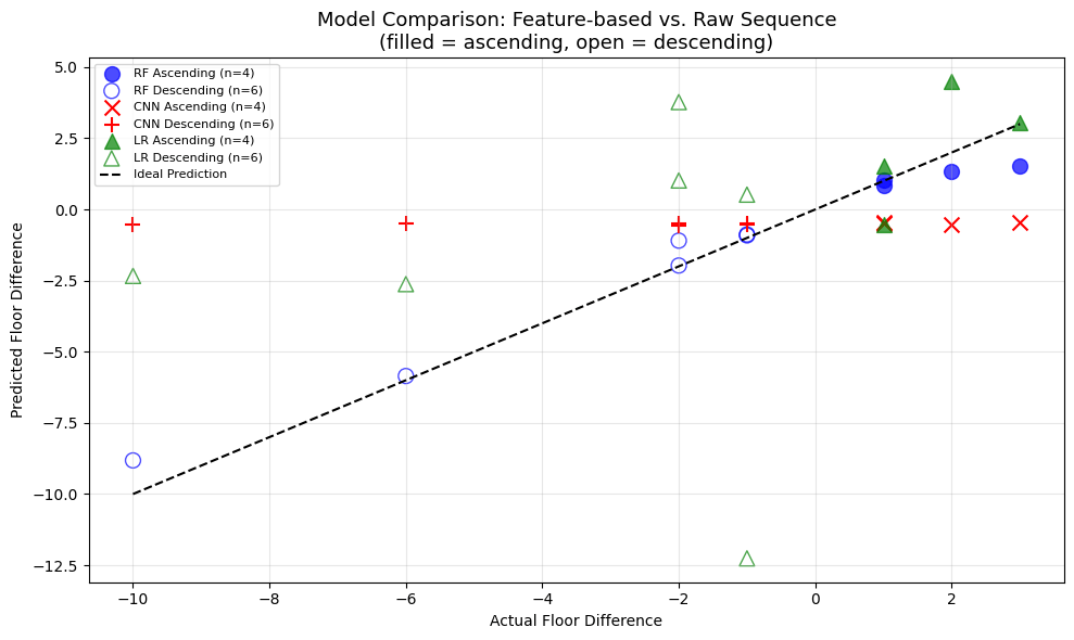
A scatter plot comparing the actual and anticipated floor differences for both models on the held-out test set is shown in Figure 3, offering a clear visual comparison of their predictive ability. The basic distinction between the two methods is demonstrated by the striking visual contrast in Figure 3. Within this pilot test set, the Random Forest predictions (blue circles) form a tight diagonal cluster along the optimum prediction line. As a sign of extreme underfitting on sparse training data, the CNN predictions (red crosses) are crowded horizontally close to zero, indicating that the model has collapsed to predicting a constant value.

Comparative Analysis

Model	MAE	RMSE	R²	Status
A	0.48 floors (~1.6 m)	0.70 floors (~2.3 m)	0.96	✓ Optimal
B	2.78 floors (~9.2 m)	3.51 floors (~11.6 m)	−0.06	× Failed
0: Linear Regression	3.72 floors (~12.3 m)	5.01 floors (~16.5 m)	-0.81	× Failed
Barometer*	1.2 floors (3–5 m error)	~1.50 floors (~5.0 m)†	~0.74†	~ Baseline
GPS*	>3.0 floors (>10 m)	~4.38 floors (~14.5 m)†	~-1.17†	× Unusable

Key Finding: Within this pilot dataset, a clear advantage of physics-informed feature engineering over end-to-end deep learning was observed. Additionally, the Random Forest model achieved sub-floor accuracy (0.48 floors, ~1.6m) which compares favorably with the standard 3-5 meter (1.0-1.5 floor) error margin of barometer sensors, though direct comparison requires caution given the small test set.

Discussion

Interpretation of Feature-Based Model Success

The Random Forest model’s promising preliminary performance (MAE = 0.48 floors, ~1.6 m, R² = 0.96, test N=10) can be attributed to two synergistic factors:

Physical alignment with kinematics: Basic elevator motion physics are immediately encoded in the retrieved features. Despite having little training data, the model may generalize across various elevator kinds and buildings thanks to the strong inductive bias provided by the relationship z ≈ vₘₐₓ × Δt. This remains to be confirmed with larger and more diverse datasets.

Ensemble robustness: The model is intrinsically stable and resistant to overfitting on short datasets since Random Forest’s averaging across 100 decision trees decreased prediction variance. The Random Forest outperformed the linear regression baseline (MAE = 3.72 floors, R² = −0.81) by 3.24 floors, confirming that the nonlinear ensemble structure adds substantial value over a simple linear mapping of the feature set.

Interpretation of CNN Failure and Small-Data Deep Learning

The poor performance of the specific CNN configuration tested here (MAE = 2.78, ~9.2m, R2 = -0.06) is consistent with the challenges of applying deep learning in small-data regimes, but should not be interpreted as evidence that deep learning is categorically unsuitable for this problem. The ~200 learnable parameters of the model faced a highly unfavourable input dimensionality-to-sample ratio (3,000 input dimensions to 40 training samples, a 75 :1 ratio), which is a known challenge for convolutional architectures^21,24. However, only a single fixed architecture was tested — with a fixed input length of 3,000 samples (requiring zero-padding), a fixed learning rate of 0.001, and 100 training epochs. Simpler alternatives such as a single-layer CNN, a fully connected network operating on the raw sequence, or data augmentation strategies (e.g., time-shifting, amplitude scaling, synthetic noise injection) were not evaluated. It is therefore possible that a more carefully tuned or augmented deep learning approach could perform better on this dataset, and the observed performance gap should be attributed specifically to this untested configuration on this small dataset rather than to deep learning in general.

Comparison with Baseline Methods

Our accelerometer-based approach (MAE = 0.48 floors, ~1.6 m vertical error, assuming 3.3m inter-floor spacing) shows preliminary evidence of performance comparable to or better than barometric methods even under ideal laboratory conditions (3–5 m error, or 1.0–1.5 floors), while potentially offering the following advantages pending larger-scale validation:

Environmental independence: Unlike barometric sensors, which are unreliable in realistic scenarios with HVAC systems and weather fluctuations⁴, accelerometer-based estimation is not subject to pressure variations.

Potential hardware compatibility: The technique requires only an accelerometer, which is found in almost all smartphones. This reduces reliance on barometric sensors, which are absent from many low-cost devices.

Potentially Superior to GPS: Even outside, GPS vertical inaccuracies are more than 10 meters, and within, they are completely unusable, making it generally unsuitable for determining floor level.

Potential Future Applications

For many real-world applications, the 0.48-floor (~1.6 m) average error observed in this pilot suggests potential to meet practical requirements:

In 9 out of 10 test cases, predictions were within ±1 floor of ground truth. This figure should be interpreted with caution given the very small test set size.

Elevator-Specific Insights

Per-elevator performance was qualitatively examined but is not reported in detail here, as with approximately 10 rides per elevator the per-elevator sample sizes are too small to draw reliable quantitative conclusions. No gross failures were observed across any single elevator, which is weakly consistent with some degree of robustness to variation in elevator parameters (acceleration profiles, motor types, cabin weights). However, with N = 50 total samples collected by a single user under controlled posture conditions, these observations cannot be taken as confirmation of broad generalizability; multi-building, multi-user validation with sufficient rides per elevator is needed before any per-elevator conclusions can be drawn.

Limitations and Future Directions

Several limitations warrant consideration:

Single-participant data: All 50 rides were collected by a single 17-year-old researcher holding the phone vertically in a stationary posture. Variability in user age, mobility, phone grip, body movement, and phone placement (e.g., pocket, bag, hand) was not examined. These factors are likely to introduce significant signal variability in real-world deployment and must be addressed through multi-user validation before any practical application can be considered.

Conclusions

This study in five commercial elevators showed that using only smartphone accelerometer data, physics-informed feature engineering and Random Forest regression produced promising preliminary results for floor-level estimation (MAE = 0.48 floors, vertical error ~1.6 m assuming 3.3 m inter-floor spacing) without the need for barometric sensors or GPS infrastructure. Comparative analysis is consistent with the idea that “good features outweigh complex models when data is scarce” by confirming that feature-based machine learning may outperform end-to-end deep learning in small-data regimes (N = 50) in this pilot. This finding should be interpreted narrowly: it reflects the performance of one untested CNN configuration relative to a well-tuned feature-based approach, and does not constitute a general conclusion about deep learning versus feature engineering. Alternative CNN designs, simpler sequence models, or data augmentation strategies were not explored and may yield different outcomes.

The suggested approach shows potential advantages over current methods: it operates on hardware commonly found in smartphones, may outperform GPS for indoor vertical positioning, and achieved accuracy comparable to or better than barometric systems in this pilot even under ideal conditions while not being subject to environmental pressure fluctuations. However, as all data were collected in commercial office buildings, the approach should not yet be considered a general solution for multistory buildings broadly. Because of these characteristics, the system shows preliminary promise for location-aware services, asset tracking, and emergency response in controlled conditions, though practical deployment would require further research including on-device runtime evaluation, real-time feature extraction testing, and multi-user validation.

Future research directions

include: (1) enlarging the dataset to 300–500 samples to see if deep learning techniques can match or surpass Random Forest performance at scale²⁵; (2) validating the results across multiple users to analyze generalization across various phone handling behaviors; (2b) implementing leave-one-elevator-out and leave-one-building-out evaluation schemes to properly assess cross-elevator and cross-building generalizability; (3) extending to other vertical modalities (stairs, ramps, escalators) for a thorough vertical motion classification²⁶; (4) evaluating on-device runtime, inference latency, and battery impact as necessary prerequisites before any real-time smartphone deployment can be considered; and (5) exploring adaptation strategies for irregular floor spacing in buildings.

This work contributes to the field of infrastructure-free interior positioning and lays the groundwork for future advancements in smartphone-based vertical localization by proving initial evidence for the feasibility of accelerometer-only floor estimation.

Acknowledgments

I acknowledge the open-source communities behind Python, scikit-learn, TensorFlow, and phyphox, whose tools made this research possible. Special thanks to my research advisors for guidance on feature engineering methodology and statistical analysis.

Appendix A: Data Collection Protocol
A.1 Step-by-Step Procedure
Identify starting floor and verify using building directory and elevator display
Launch phyphox application (version 1.2.0) and navigate to “Acceleration (without g)” experiment
Press record button to begin data collection at 100 Hz
Enter elevator and maintain stationary posture holding phone vertically
Travel to destination floor without intermediate stops (Off-peak hours were chosen to minimise interruptions; any interrupted ride was immediately discarded and repeated)
Stop recording in phyphox and export data via “Share” function as CSV file
Exit elevator after doors open
Rename file following convention: [Elevator][Start]-[End]-[Trial].xls
Document metadata (date, time, building, elevator model) in research notebook
Repeat across all target floor combinations and elevator units

Appendix B: Complete Python Implementation
B.1 Google Colab Notebook Code
The complete implementation is provided below. This code can be executed in Google Colab by uploading the CSV dataset to Google Drive and adjusting the base_path variable.

Listing 1: Data Preprocessing and Feature Extraction
# Mount Google Drive
from google.colab import drive
drive.mount('/content/drive')

import os, re
import pandas as pd
import numpy as np
from scipy.integrate import cumulative_trapezoid
from scipy.signal import butter, filtfilt, medfilt

class ElevatorTrimmerRobust:
    def __init__(self, fs=100.0, threshold=0.06,
                 min_duration_sec=1.0, padding_sec=1.5):
        self.fs = fs
        self.threshold = threshold
        self.min_duration_sec = min_duration_sec
        self.padding_sec = padding_sec

    def load_and_trim(self, file_path):
        try:
            df = pd.read_excel(file_path)
            t  = df.iloc[:, 0].values.astype(float)
            az = df.iloc[:, 3].values.astype(float)
        except Exception as e:
            return None, None

        t = t - t[0]
        b, a = butter(2, 2.0 / (0.5 * self.fs), btype='low')
        az_filt = filtfilt(b, a, az) - np.mean(az)
        az_despike = medfilt(az_filt, kernel_size=9)

        mask = np.abs(az_despike) > self.threshold
        diff = np.diff(np.concatenate(([False], mask, [False])).astype(int))
        starts = np.where(diff == 1)[0]
        ends   = np.where(diff == -1)[0]

        if len(starts) == 0:
            return None, None

        best_segment = None
        for s, e in zip(starts, ends):
            if (e - s) / self.fs >= self.min_duration_sec:
                if best_segment is None:
                    best_segment = [s, e]
                else:
                    best_segment[1] = e

        if best_segment is None:
            return None, None

        pad = int(self.padding_sec * self.fs)
        trim_start = max(0, best_segment[0] - pad)
        trim_end   = min(len(t), best_segment[1] + pad)
        t_trim  = t[trim_start:trim_end]
        az_trim = az[trim_start:trim_end]
        if len(t_trim) > 0:
            t_trim = t_trim - t_trim[0]
        return t_trim, az_trim

def create_dataset(base_path):
    trimmer = ElevatorTrimmerRobust()
    dataset = []
    for elevator in ['A','B','C','D','E']:
        for direction in ['ascend','descend']:
            folder = os.path.join(base_path, elevator, direction)
            if not os.path.exists(folder): continue
            for fname in [f for f in os.listdir(folder) if f.endswith('.xls')]:
                m = re.search(r'([A-E])(\d+)-(\d+)-(\d+)', fname)
                if not m: continue
                start_floor = int(m.group(2))
                end_floor   = int(m.group(3))
                t_trim, az_trim = trimmer.load_and_trim(os.path.join(folder, fname))
                if t_trim is None: continue
                duration = t_trim[-1] - t_trim[0]
                v = cumulative_trapezoid(az_trim, t_trim, initial=0)
                dataset.append({
                    'elevator_id': elevator, 'direction': direction,
                    'filename': fname, 'start_floor': start_floor,
                    'end_floor': end_floor,
                    'floor_diff': end_floor - start_floor,
                    'duration': duration,
                    'acc_max': np.max(az_trim), 'acc_min': np.min(az_trim),
                    'acc_energy': np.mean(np.abs(az_trim)),
                    'vel_max': np.max(v), 'vel_min': np.min(v),
                    'dist_approx': cumulative_trapezoid(v, t_trim, initial=0)[-1]
                })
    return pd.DataFrame(dataset)

base_path = '/content/drive/MyDrive/research/data'
df = create_dataset(base_path)
df.to_csv('/content/drive/MyDrive/research/dataset.csv', index=False)
print(f'Dataset created: {len(df)} samples')

Listing 2: Model Training and Evaluation
from sklearn.linear_model import LinearRegression
from sklearn.ensemble import RandomForestRegressor
from sklearn.metrics import mean_absolute_error, r2_score, mean_squared_error
from sklearn.model_selection import train_test_split
import matplotlib.pyplot as plt


# Load dataset
df = pd.read_csv('/content/drive/MyDrive/research/dataset.csv')
X = df[['duration','acc_max','acc_min','acc_energy','vel_max','vel_min','dist_approx']].values
y = df['floor_diff'].values

# Train-test split
direction_labels = df['direction'].values
indices = np.arange(len(y))
X_train, X_test, y_train, y_test, idx_train, idx_test = train_test_split(
    X, y, indices, test_size=0.2, random_state=42,
    stratify=direction_labels
)

# ===== Model 0: Linear Regression Baseline =====
print("\n[Model 0] Training Linear Regression baseline...")
lr_model = LinearRegression()
lr_model.fit(X_train, y_train)
y_pred_lr = lr_model.predict(X_test)
 
mae_lr  = mean_absolute_error(y_test, y_pred_lr)
rmse_lr = np.sqrt(mean_squared_error(y_test, y_pred_lr))
r2_lr   = r2_score(y_test, y_pred_lr)
print(f"  >> Linear Regression MAE:  {mae_lr:.2f} floors")
print(f"  >> Linear Regression RMSE: {rmse_lr:.2f} floors")
print(f"  >> Linear Regression R2:   {r2_lr:.2f}")

# Train Random Forest

rf = RandomForestRegressor(n_estimators=100, max_depth=10,
                           min_samples_leaf=2, random_state=42)
rf.fit(X_train, y_train)

# Predict
y_pred_rf = rf.predict(X_test)

# Evaluate
mae_rf = mean_absolute_error(y_test, y_pred_rf)
rmse_rf = np.sqrt(mean_squared_error(y_test, y_pred_rf))
r2_rf = r2_score(y_test, y_pred_rf)
 
print(f"Random Forest MAE: {mae_rf:.2f} floors")
print(f"Random Forest RMSE: {rmse_rf:.2f} floors")
print(f"Random Forest R2: {r2_rf:.2f}")

# ===== Directional Performance Breakdown =====
direction_test = df['direction'].values[idx_test]
asc_mask  = direction_test == 'ascend'
desc_mask = direction_test == 'descend'
 
mae_rf_asc  = mean_absolute_error(y_test[asc_mask],  y_pred_rf[asc_mask])  \
              if asc_mask.sum()  > 0 else float('nan')
mae_rf_desc = mean_absolute_error(y_test[desc_mask], y_pred_rf[desc_mask]) \
              if desc_mask.sum() > 0 else float('nan')
 
print(f"\n[Model A] Random Forest Directional MAE:")
print(f"  >> Ascending  (n={asc_mask.sum()}):  MAE = {mae_rf_asc:.2f} floors")
print(f"  >> Descending (n={desc_mask.sum()}): MAE = {mae_rf_desc:.2f} floors")
 
# ===== Summary =====
print(f"\n[Model 0] Linear Regression MAE: {mae_lr:.2f} | R2: {r2_lr:.2f}")
print(f"[Model A] Random Forest     MAE: {mae_rf:.2f} | R2: {r2_rf:.2f}")

Listing 3: CNN Model Implementation
from tensorflow.keras.models import Sequential
from tensorflow.keras.layers import Conv1D, MaxPooling1D, \
     Dropout, GlobalAveragePooling1D, Dense
from tensorflow.keras.optimizers import Adam
from tensorflow.keras.regularizers import l2
from tensorflow.keras.preprocessing.sequence import pad_sequences
 
# Prepare sequence data
trimmer = ElevatorTrimmerRobust()
sequences = []
for idx, row in df.iterrows():
    file_path = os.path.join(base_path, row['elevator_id'],
                             row['direction'], row['filename'])
    _, az_trim = trimmer.load_and_trim(file_path)
    if az_trim is not None:
        sequences.append(az_trim)
    else:
        sequences.append(np.zeros(100))
 
MAX_LEN = 3000
X_seq = pad_sequences(sequences, maxlen=MAX_LEN,
                      dtype='float32', padding='post')
X_seq = X_seq.reshape((X_seq.shape[0], X_seq.shape[1], 1))
 
# Split
X_seq_train, X_seq_test = X_seq[idx_train], X_seq[idx_test]
 
# Build CNN
cnn = Sequential([
    Conv1D(8, kernel_size=10, activation='relu',
           input_shape=(MAX_LEN, 1),
           kernel_regularizer=l2(0.01)),
    MaxPooling1D(pool_size=4),
    Dropout(0.3),
    Conv1D(16, kernel_size=5, activation='relu',
           kernel_regularizer=l2(0.01)),
    MaxPooling1D(pool_size=4),
    Dropout(0.3),
    GlobalAveragePooling1D(),
    Dense(16, activation='relu', kernel_regularizer=l2(0.01)),
    Dense(1, activation='linear')
])
 
cnn.compile(optimizer=Adam(learning_rate=0.001),
            loss='mse', metrics=['mae'])
 
# Train
history = cnn.fit(X_seq_train, y_train, epochs=100,
                  batch_size=8, validation_split=0.1,
                  verbose=0)
 
# Predict
y_pred_cnn = cnn.predict(X_seq_test).flatten()
 
# Evaluate
mae_cnn = mean_absolute_error(y_test, y_pred_cnn)
r2_cnn = r2_score(y_test, y_pred_cnn)
 
print(f"1D CNN MAE: {mae_cnn:.2f} floors")
print(f"1D CNN R2: {r2_cnn:.2f}")
 
# ===== Scatter Plot with Directional Markers =====
fig, ax = plt.subplots(figsize=(10, 6))
 
# Random Forest: filled circles (asc), open circles (desc)
ax.scatter(y_test[asc_mask], y_pred_rf[asc_mask],
           color='blue', marker='o', s=100, alpha=0.7,
           label=f'RF Ascending (n={asc_mask.sum()})')
ax.scatter(y_test[desc_mask], y_pred_rf[desc_mask],
           color='blue', marker='o', s=100, alpha=0.7,
           facecolors='none', edgecolors='blue',
           label=f'RF Descending (n={desc_mask.sum()})')
 
# CNN: x markers (asc), + markers (desc)
ax.scatter(y_test[asc_mask], y_pred_cnn[asc_mask],
           color='red', marker='x', s=100,
           label=f'CNN Ascending (n={asc_mask.sum()})')
ax.scatter(y_test[desc_mask], y_pred_cnn[desc_mask],
           color='red', marker='+', s=100,
           label=f'CNN Descending (n={desc_mask.sum()})')
 
# Linear Regression: filled triangles (asc), open triangles (desc)
ax.scatter(y_test[asc_mask], y_pred_lr[asc_mask],
           color='green', marker='^', s=100, alpha=0.7,
           label=f'LR Ascending (n={asc_mask.sum()})')
ax.scatter(y_test[desc_mask], y_pred_lr[desc_mask],
           color='green', marker='^', s=100, alpha=0.7,
           facecolors='none', edgecolors='green',
           label=f'LR Descending (n={desc_mask.sum()})')
 
# Ideal line
min_val = min(y_test.min(), y_pred_rf.min(), y_pred_cnn.min())
max_val = max(y_test.max(), y_pred_rf.max(), y_pred_cnn.max())
ax.plot([min_val, max_val], [min_val, max_val], 'k--',
        label='Ideal Prediction')
 
ax.set_title('Model Comparison: Feature-based vs. Raw Sequence\n'
             '(filled = ascending, open = descending)', fontsize=13)
ax.set_xlabel('Actual Floor Difference')
ax.set_ylabel('Predicted Floor Difference')
ax.legend(fontsize=8)
ax.grid(True, alpha=0.3)
plt.tight_layout()
plt.show()


B.2 Notes on Reproducibility
1.	Upload the elevator dataset to Google Drive following the directory structure described in Methods.
2.	Open a new Google Colab notebook and paste the code above.
3.	Adjust the base_path variable to match your Google Drive directory.
4.	Execute cells sequentially.
5.	Random seed (random_state=42) ensures reproducible train-test splits.

All experiments were conducted using Google Colab's free tier (CPU runtime). Total computation time was approximately 5 minutes for the complete pipeline.

References

1. B. Hofmann-Wellenhof, H. Lichtenegger, J. Collins. GPS: Theory and Practice. Springer Science & Business Media, 5th ed., 2012. [↩]
2. R. Harle. A survey of indoor inertial positioning systems for pedestrians. IEEE Communications Surveys & Tutorials, vol. 15, no. 3, pp. 1281–1293, 2013. https://doi.org/10.1109/SURV.2012.121912.00075. [↩]
3. S. Manivannan, S. Wisely, R. R. Swarup. Challenges and potential of using barometric pressure for mobile sensing. Proceedings of the 2020 IEEE International Conference on Acoustics, Speech and Signal Processing. 2020. [↩]
4. H. Ye, T. Liu, X. Tan, J. Yang, G. Mao. HiMeter: Telling you the height rather than the altitude. Sensors. Vol. 18, p. 1870, 2018. https://doi.org/10.3390/s18061870. [↩] [↩] [↩]
5. W. Jaworski, P. Wilk, P. Zborowski, W. Chmielowiec. A comprehensive algorithm for vertical positioning in multi-building environments as an advancement in indoor floor-level detection. Scientific Reports, vol. 14, p. 13996, 2024. https://doi.org/10.1038/s41598-024-64824-9. [↩]
6. L. Xia, Z. Tian, Y. Li, D. Ma. Barometric altimetry for indoor localization: A comprehensive study. IEEE Sensors Journal. Vol. 19, pp. 748–759, 2019. https://doi.org/10.1109/JSEN.2018.2878688. [↩]
7. Y. Jiang, X. R. Pan, K. Li, Q. Lv, R. P. Dick, M. Hannigan, Q. Shao. Towards fingerprint-free floor localization using barometric pressure sensor. Proceedings of the 2014 International Conference on Indoor Positioning and Indoor Navigation. 2014. [↩]
8. X. Li, Y. Wang, C. Khedo, Y. Wang. SmartLoc: push the limit of the inertial sensor for indoor localization. Proceedings of the 20th Annual International Conference on Mobile Computing and Networking. 2014. [↩]
9. Z. Zhu, J. Liu, X. Niu, Z. Gao. Height estimation for floor identification in elevator and escalator scenarios based on smartphones built-in IMU. IEEE Sensors Journal, 2024. https://doi.org/10.1109/JSEN.2024.3444918. [↩]
10. R. Gonçalves, J. Sousa, F. Meneses, A. Moreira. Human activity recognition for indoor localization using smartphone inertial sensors. Sensors, vol. 21, no. 18, p. 6316, 2021. https://doi.org/10.3390/s21186316. [↩] [↩]
11. T. Guo, J. Yin, W. Wang, M. Jia, P. Yang. A comprehensive study of smartphone-based indoor activity recognition via XGBoost. IEEE Access, vol. 7, pp. 80027–80042, 2019. https://doi.org/10.1109/ACCESS.2019.2925534. [↩]
12. H. Liu, H. Darabi, P. Banerjee, J. Liu. Survey of wireless indoor positioning techniques and systems. IEEE Transactions on Systems, Man, and Cybernetics. Vol. 37, pg. 1067–1080, 2007, https://doi.org/10.1109/TSMCC.2007.905127. [↩]
13. A. Nessa, B. Adhikari, F. Hussain, X. N. Fernando. A survey of machine learning for indoor positioning. IEEE Access, vol. 8, pp. 214945–214965, 2020. https://doi.org/10.1109/ACCESS.2020.3039271. [↩]
14. T. Yang, A. Cabani, H. Chafouk. A survey of recent indoor localization scenarios and methodologies. Sensors. Vol. 21, pg. 8086, 2021, https://doi.org/10.3390/s21238086. [↩]
15. J. Shang, Y. Wu. Overview of WiFi fingerprinting-based indoor positioning. IET Communications, vol. 16, no. 6, pp. 598–618, 2022. https://doi.org/10.1049/cmu2.12386. [↩]
16. L. Breiman. Random forests. Machine Learning, vol. 45, no. 1, pp. 5–32, 2001. https://doi.org/10.1023/A:1010933404324. [↩] [↩]
17. J. Stauffer, S. Brunner, K. Dorner, A. Rittenschober. phyphox: physical phone experiments. https://phyphox.org, 2022. [↩]
18. Z. Zhu, J. Liu, X. Niu, Z. Gao. Height estimation for floor identification in elevator and escalator scenarios based on smartphones built-in IMU. IEEE Sensors Journal, 2024. https://doi.org/10.1109/JSEN.2024.3444918. [↩]
19. F. Pedregosa, G. Varoquaux, A. Gramfort, V. Michel, B. Thirion, O. Grisel, M. Blondel, P. Prettenhofer, R. Weiss, V. Dubourg, J. Vanderplas, A. Passos, D. Cournapeau, M. Brucher, M. Perrot, E. Duchesnay. Scikit-learn: Machine learning in Python. Journal of Machine Learning Research, vol. 12, pp. 2825–2830, 2011. [↩]
20. C. A. Ronao, S.-B. Cho. Human activity recognition with smartphone sensors using deep learning neural networks. Expert Systems with Applications, vol. 59, pp. 235–244, 2016. https://doi.org/10.1016/j.eswa.2016.04.032. [↩]
21. H. I. Fawaz, G. Forestier, J. Weber, L. Idoumghar, P.-A. Muller. Deep learning for time series classification: a review. Data Mining and Knowledge Discovery, vol. 33, no. 4, pp. 917–963, 2019. https://doi.org/10.1007/s10618-019-00619-1. [↩] [↩]
22. C. A. Ronao, S.-B. Cho. Human activity recognition with smartphone sensors using deep learning neural networks. Expert Systems with Applications. Vol. 59, pg. 235–244, 2016, https://doi.org/10.1016/j.eswa.2016.04.032. [↩]
23. H. I. Fawaz, G. Forestier, J. Weber, L. Idoumghar, P.-A. Muller. Deep learning for time series classification: a review. Data Mining and Knowledge Discovery. Vol. 33, pg. 917–963, 2019, https://doi.org/10.1007/s10618-019-00619-1. [↩]
24. D. Anguita, A. Ghio, L. Oneto, X. Parra, J. L. Reyes-Ortiz. A public domain dataset for human activity recognition using smartphones. Proceedings of the European Symposium on Artificial Neural Networks (ESANN). pg. 437–442, 2013. [↩]
25. K. Kim, J. Park, S. Kim. Deep learning-based multi-floor indoor localization using smartphone IMU sensors with 3D location initialization. IEEE Access, vol. 13, 2025. https://ieeexplore.ieee.org/document/11029293. [↩]
26. C. De Cock, W. Joseph, L. Martens, J. Trogh, D. Plets. Multi-floor indoor pedestrian dead reckoning with a backtracking particle filter and Viterbi-based floor number detection. Sensors, vol. 21, no. 13, pp. 4565–4593, 2021. https://doi.org/10.3390/s21134565. [↩]