
Abstract
This paper investigates whether Artificial Intelligence (AI) can predict whether a sequence of swaps applied to a finite set produces a complete cycle, defined as a permutation whose disjoint cycle decomposition consists of a single  -cycle. The task is useful for testing whether neural networks can learn combinatorial structure from permutation-based sequence data. The objective of this investigation was to evaluate the effectiveness of Gated Recurrent Unit (GRU)-based models in predicting complete-cycle structure from generated swap sequences. A fully synthetic dataset of 30,000 swap sequences was created by randomly sampling permutation sizes from
 , and swap sequence lengths from
 . Each sequence was applied to the identity permutation and deterministically labelled according to whether the resulting permutation formed a complete cycle. Adam and Stochastic Gradient Descent (SGD) were compared across learning rates, and Adam with a learning rate of 0.0028 was selected for the final repeated layer-sweep experiments. Model performance was evaluated using test accuracy and F1 score. Results showed that GRU models learned meaningful structure from swap sequences, but increasing depth did not consistently improve performance. Kruskal-Wallis H tests showed that accuracy and F1 score differed significantly across layer depths, while Dunn’s post-hoc tests indicated that Layers 1-7 formed a statistically similar performance band before performance declined in deeper models. These findings suggest that increased architectural complexity does not necessarily improve performance on this task. Future research could extend the model to predict full cycle decompositions rather than only binary complete-cycle labels.
Keywords: Machine learning, stochastic gradient descent, Adam, Recurrent Neural Network, Long Short-Term Memory, feed forward, sigmoid activation function, training data, swaps, sequence.
Introduction
We aim at answering the question of: Which neural network architecture achieves the best accuracy and computationally efficient prediction of cycle structure for generated swap permutations? The cycle structure of a permutation is not an artificial target. Genome rearrangement problems can be represented as sorting a permutation by transpositions, where lower bounds on evolutionary distance are derived from cycle structures in associated representations of the permutation1. In sorting theory, the minimum number of transpositions needed to sort a permutation equals n minus its number of cycles, so counting cycles is exactly the cost of sorting by swaps. In the study of shuffling, Diaconis and Shahshahani showed how many random transpositions are needed to mix a deck2. Our task asks whether a small recurrent network can pick up this kind of algebraic structure from examples alone. This places the paper within neural algorithmic reasoning, which studies how neural networks can learn to execute algorithmic computation from data3.
It is of significance to understand how different neural network architectures compare and test for the optimal learning rate and optimization algorithm to enable effective generalization to longer swaps and larger permutations. This contributes to a broader understanding of neural network architectures as learned algorithms for combinatorial reasoning. Additionally, the research is useful in comparing how neural network architectures learn and generalize compositional, group-structured rules from sequences of swaps.
The scope of the study is limited to permutations made by applying finite sequences of paired swaps to the permutation, with the prediction task framed as a binary classification problem. The analysis considers Gated Recurrent Unit (GRU) architectures trained on synthetically generated data, and evaluates performance under fixed computational constraints, including bounded permutation size, sequence length, and training epochs.
This investigation aims to evaluate the ability of GRU-based neural networks to predict whether a generated swap sequence produces a complete cycle. A swap ( ) is a transposition operation that exchanges the elements in positions
 and
 . A sequence of swaps itself is not a permutation, instead when the swaps are applied to the identity permutation 1, 2, . . . ., n], they produce a final permutation
 . In this paper, a permutation is defined a complete cycle if its disjoint cycle decomposition consists of a single cycle of length . Repeatedly, applying the permutation from any starting position visits all positions exactly once before returning to the starting position.
For example, the permutation  is a complete cycle because repeated application cycles through all three positions before returning to the start. This notation means that position 1 maps to 2, position 2 maps to 3, and position 3 maps back to 1. The task becomes more difficult as the permutation size and swap-sequence length
 increase, because the final permutation must first be generated from the swap sequence and then checked for cycle structure. In this investigation, was randomly sampled from
 and was randomly sampled from
 .
Although previous studies address data with permutation-related characteristics, they focus on different learning problems than the prediction of cycle structure in swap=generated permutations considered in this work. Zhang & Bloom investigated neural network architectures used for modelling sequential data and found that recurrent and convolutional neural networks (RNN, CNN) were sub-optimal because of invariance to cyclic phase shifts of periodic data4. Instead, cyclical-permutation invariant networks (iTCN/iResNet) which are invariant to phase shifts in the input data, outperformed both non-invariant versions of the same network. This was achieved by representing the data in phase space, performing convolutions in polar coordinates, and global pooling over all phases. The results included approximately 93% accuracy on variable star classification.
Furthermore, a study in China by Huang et alutilized an adjacency matrix to encode neighbourhood structures and analysed permutation-sensitive GNNs with RNN aggregators, proposing PG-GNN. This model achieved 76.8-80.9% accuracy on graph-classification benchmarks from the TUDataset5. Its permutation-sensitive aggregation mechanism via permutation groups captured pairwise correlations between neighbouring nodes while maintaining linear sampling complexity.
Moreover, Kimura et al reviewed a broad range of permutation-invariant neural network architecture designed for set-structured data6. The study highlighted limitations of conventional machine-learning algorithms that assume the inputs are represented in a vector-based format. It also discussed architectures such as DeepSets and Transformers, which are designed to accommodate set inputs and enable more effective representation and processing of set structures.
These studies solve adjacent problems, and none of them classify a group-theoretic property of a composed permutation from its generating swaps. Zhang and Bloom build networks that are invariant to cyclic shifts of periodic signals; our sequences are not periodic, but their result shows that matching the architecture to a symmetry of the data pays off. Huang et al. treat permutations of graph neighborhoods, where order should not matter. Kimura et al. survey set-structured inputs, where order must not matter at all. Our task is the opposite case: the order of the swaps is the signal. We therefore use a plain sequence model and measure how much of the algebraic structure it can absorb, rather than building the structure into the architecture.
| Study | Input | Task | How this paper differs |
| Zhang and Bloom (2021) | Periodic light curves | Variable star classification | We classify an algebraic property, not a periodic signal. |
| Huang et al (2022) | Graphs | Graph classification | Our input is an ordered swap sequence, not a neighborhood set. |
| Kimura et al (2024) | Sets | Survey of permutation-invariant networks | Our target depends on order, so invariance would destroy the label. |
| This paper | Swap Sequences | Binary n-cycle classification | Controlled GRU depth comparison on a group-structured rule. |
The contribution of this paper is a controlled empirical comparison of GRU depths, optimizers, and learning rates for binary cycle classification on synthetic swap sequences. We do not claim new architecture or a new learning method. There is substantial prior work on permutation learning, including set-based networks, permutation-equivariant networks, and graph neural networks for combinatorial problems. Our study is narrower: it asks how far a plain recurrent classifier gets on one sharply defined group-theoretic property, and it reports the answer using repeated trials, standard deviations, and statistical tests. Table 2 displays the variable definitions.
| Model | Optimization | Data |
|---|---|---|
 — Weight matrix |  — Loss function | — Size of elements |
 — Layer number in a neural network |  — First moment estimate mean |  — Time steps in a sequence |
 — Sigmoid activation function |  — Second moment estimate mean | — Number of swaps in a sequence |
 — Hyperbolic tangent activation function |  — Decay rate for first moment |  — Number of training samples |
 — Bias vector |  — Decay rate for squared gradients | |
 — Hidden state |  — Updated parameter value | |
 — Cell state |  — Learning rate | |
 — Candidate memory |  — Small constant to prevent division by 0 | |
 — Forget gate |  — Gradient | |
| — Input gate | ||
 — Reset gate | ||
 — Update gate | ||
 — Candidate hidden state | ||
 — Output activation | ||
 — Output gate |
Methods
Materials
All experiments were conducted in Python using Visual Studio Code on a local CPU system. No ethical concerns arose, as no human or personal data were involved. Deep learning models were implemented in PyTorch, utilizing automatic differentiation, computation graphs7. GRU-based models, through nn.GRU, were used to process sequential swap data, with variable length handling implemented through batching, padding and packed padded sequences. Binary classification was performed using BCEWithLogitsLoss, which combines the sigmoid transformation and binary cross-entropy loss in a numerically stable form. During evaluation, logits were converted to probabilities using a sigmoid function before applying the selected threshold.
The experiment used a naturally generated dataset of 30,000 swap-sequence samples. For each sample, the permutation size was randomly selected from  , and the number of swaps was randomly selected from
 . The dataset was split into training, validation, and testing sets using a 70:15:15 ratio. Random seeds were controlled using Python’s random, NumPy, and PyTorch seed setting functions to improve reproducibility across repeated trials.
Training used gradient-based optimizers, including Adam and stochastic gradient descent, during preliminary optimizer and learning-rate testing. Based on these tests, Adam with a learning rate of 0.0028 was selected for the final repeated layer-sweep experiments. The final experiments used batch size 32, hidden size 64, embedding dimension 16, dropout 0.2, maximum 50 epochs, and early-stopping patience of 5.
Mini batch loading and shuffling were handled using DataLoader. Model performance was evaluated using precision, recall, F1 score, and confusion matrices through scikit-learn. Training dynamics and learning rate analyses were visualized using Matplotlib, with additional numerical computations performed using NumPy and SciPy.
To assess whether test accuracy and F1 score differed significantly across the ten GRU layer depths, Shapiro-Wilk tests were first used to assess normality within each layer group, and Levene’s test was used to assess homogeneity of variance across groups. Because normality was violated in several layer groups and Levene’s test indicated unequal variance for F1 score, the Kruskal-Wallis H test was used as the primary non-parametric omnibus test. A one-way ANOVA was also computed as a robustness check. Effect sizes were reported using epsilon-squared ( ) for the Kruskal-Wallis tests. Where the omnibus test was significant, Dunn’s post-hoc test with Bonferroni correction was used for pairwise comparisons across layer depths. Statistical significance was set at
 .
Neural Network Architecture:
In terms of deciding the neural network architecture, we decided to use a Gated Recurrent Unit (GRU) architecture over the Feed Forward (FF), vanilla Recurrent Neural Network (RNN) and Long Short-Term Memory (LSTM). A FF network is a multilayer perceptron in which information only flow from the input layer to the output layer, so later layers do not give any feedback to the previous layers8. Therefore, sequential data is one of the FF’s limitations, as there is no storage or memory of previous inputs.
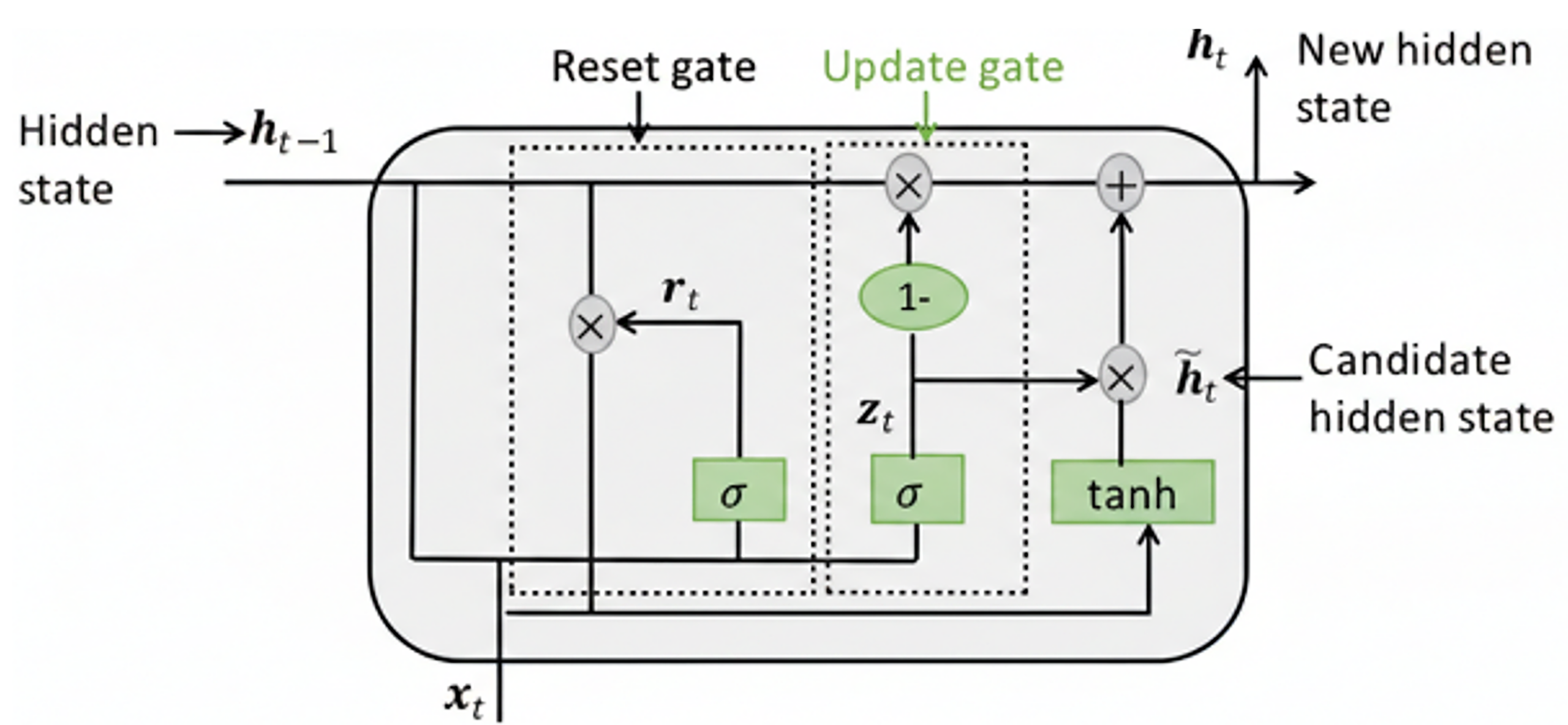
LSTMs, introduced by Hochreiter and Schmidhuber, and GRUs, introduced by Cho et al, are variants of RNN architecture and are widely used for modelling sequential data9,10,11. Like standard RNNs, LSTMs and GRUs retain information from past inputs, where the input can be in the form of sequential data. An RNN allows information to cycle between the network, and its hidden state  is updated for each time step . The GRU (Figure 3) updates its hidden state using two gates: the reset gate
 , which determines how much past information to forget, and the update gate
 which determines how much of the previous hidden state is retained. The candidate hidden state is computed using the reset-modified previous state, and the final hidden state is a weighted combination of the previous and candidate state.
Standard RNNs have difficulty learning long-term dependencies because gradient-based learning becomes increasingly challenging as dependencies span longer sequences (“the vanishing gradient problem”)12. LSTMs address this using gated memory cells but introduce additional complexity. However, GRU is another variant of RNN which has few gates, requires less memory and is much faster. GRUs address the vanishing gradient problem by being a simpler version of LSTMs, by combining the input and forget gates into a single update gate and joining the cell state and hidden state, resulting in fewer weights, parameters and higher efficiency.
The following equations present a simplified form for the GRU reset gate and update gate formulations outlined by Cho et al11,13.:
Equation 1 shows how the reset gate computes whether the previous memory is mostly ignored or if it is mostly retained, where  is the weight matrix of the reset gate. Equation 2 displays the update gate, where if
 , the unit is updated with new information, or else if
 , the old state is mostly preserved. Equation 3 and 4 explain how the candidate hidden state
 at time step is calculated and the final updated hidden state , respectively.
We chose to use a GRU neural network architecture over a LSTM neural network architecture because it has a faster training speed (due to the simplicity of architecture), as Yang et al reported that GRU model training speed was 29.29% faster than LSTM performing the same dataset14. Although both GRU and LSTM are effective sequence-modelling architectures, Chung et al found that while GRU could outperform LSTM in terms of convergence time and generalization on some datasets, the relative performance of GRU and LSTM depends on the dataset and corresponding task15. Therefore, a GRU was selected for this investigation due to its strong performance and computational efficiency.
Activation Functions
The GRU uses sigmoid activations in its reset and update gates because a gate needs an output in (0, 1): the value acts as the fraction of past state to keep. The candidate state uses tanh, which keeps values in (−1, 1) and centers them at zero, which stabilizes recurrent updates. The model outputs a raw logit. During training BCEWithLogits Loss applies the sigmoid transformation internally, while during evaluation the logit is converted to a probability using a sigmoid function before thresholding.
Loss Function
We used Binary Cross Entropy (BCE) loss as the model performs a binary classification task (complete cycle vs not). In implementation, PyTorch’s BCEWithLogitsLoss was used, which applies the sigmoid transformation internally to the model’s raw logit output. BCE penalizes incorrect high-confidence predictions more heavily than alternatives such as Mean Squared Error, making it well-suited for probabilistic outputs. The loss is derived from Bishop and is defined in the equation below16:
Where is the number of training examples in the batch,  is the true label for the
 sample.
 is the predicted probability that the sequence is a complete cycle, obtained by applying the sigmoid function to the model’s raw output logit.
Experiment Design
The full code used in the experiment can be found in the Appendix.
Complete Cycle Algorithm
For the complete cycle check, where the input is the permutation  and the output is True if is a single -cycle, the pseudo code is:
1. Set 
2. Create 
3. Set current index 
4. Repeat times
a. If 
b. Set 
c. Set 
d. Return True only if every position was visited and ; otherwise return False
In other words, starting from any position and repeatedly applying the permutation visits all positions exactly once before returning to the starting position. The labelling process used 2 main functions, apply_swaps and is_complete_cycle.
First, apply_swaps applied the generated swap sequence to the identity permutation  to produce the final permutation as a resultant mapping of positions. The swap sequence was interpreted using the standard right-to-left convention for permutation composition. Therefore, if the written sequence was
 then
 was applied first, followed by
 , until
 . Since GRUs process input sequences sequentially from the first swap to the last, the generated swap list was reversed before being passed into the GRU. This ensured that the model read the swaps in the same order used by the labelling algorithm.
Is_complete_cycle checked whether the final permutation was a single -cycle. The function does not take as a separate input but instead infers from the length of the permutation using len(perm). It starts at index 0 and repeatedly follows the mapping given by the permutation. If an index is visited twice before all positions are reached the function returns False, because the value will continue following the same path as it did when it was in that position the first time, which will be looped repeatedly. After steps, it returns True only if every position has been visited and the traversal has returned to the starting index.
The final permutation was used for labelling because it captures the net effect of the swap sequence, including repeated or cancelling swaps.
Imbalanced Classification Case
An imbalanced classification problem occurs when the training data provided to a machine learning (ML) model has a significantly uneven distribution of samples across different classes17. Because most randomly generated swap sequences do not yield complete cycles, the dataset became heavily skewed toward Class 0. As a result, the model defaulted to predicting Class 0 (False) for all test samples, which inflated accuracy while hiding its failure to learn patterns. This issue was identified with the F1 score because the number of positives identified was 0 and so the F1 score dropped to 0.
To address this issue, weighted losses were added for the positive examples during training, hence discouraging the model from defaulting to the majority class. Additionally, F1 score was selected based on validation sets, rather than using the fixed probability cutoff of 0.50 which may be too strict for a minority case.
Input Design
The permutation in the problem is given as a sequence of swaps in the format:

 …
 . In the code, the permutation will be a list containing each swap as an item in the list, following the same order from right to left.
E.g. [( ,
 ), (,
 )]
Training Data Generation
For Generating and Labelling One Sample, where the input is  ,
 ,
 and the output is GRU input sequence, label, , , the pseudo code is:
- Randomly choose from [2, 10]
- Randomly choose from [1, 20]
- Generate all valid swaps (i, j), where

- Randomly sample swaps to form the written sequence
- Apply S to from right to left to obtain final permutation
- Check whether is a single

- If is a single , assign label 1; otherwise assign label 0
- Reverse
 before GRU input so the model reads swaps in application order
- Store the GRU input sequence, label, , and
For each generated sample, a permutation size was randomly selected. This determined the starting identity permutation . Then was randomly selected, where represents the number of swaps in the sequence.
All valid swaps  were generated such that
 . From this list, swaps were randomly sampled to form the written swap sequence . The label was then produced by applying the swaps to the identity permutation using the right-to-left convention, producing a final permutation . If was a single -cycle, the sample was labelled 1, otherwise it was labelled 0.
Before being passed into the GRU, the written swap sequence was reversed so that the model processed the swaps in the same order used by the labelling algorithm. Each stored training sample therefore consisted of the GRU input sequence, its binary label, and metadata values and .
Padding and batching of the data are not performed during data generation, instead they occur during model training to ensure that all input sequences in a batch are of the same length, which is a requirement for GRU input.
The code uses PyTorch’s DataLoader to batch and shuffle the training data, applying padding dynamically through a custom function collate_fn.
A naturally generated dataset of 30,000 samples was created, which contained 18.15% complete-cycle examples and 81.85% non-complete cycle examples, giving an imbalance ratio of 4.51:1 between Class 0 and Class 1.
Correctness and Complexity
The algorithms are efficient because each generated sample is labelled without repeatedly applying the permutation many times. Apply_swaps cretes the identity permutation and applies each of the swaps once. Then, is_complete_cycle follows at most positions in the final permutation. Therefore, the labelling process grows linearly with the permutation size and the swap sequence length, giving a total time complexity of  for one sample.
The algorithm is correct because apply_swaps produces the final permutation generated by the written swap sequence under the right-to-left convention. The is_complete_cycle function then checks whether this final permutation is a single -cycle by following the orbit from one starting position. If all positions are visited exactly once before returning to the start, the permutation is a complete cycle.
Validation Testing and Early Stopping
The validation set was used for early stopping decisions and threshold tuning, not for training the model. During training, validation loss was monitored after each epoch to determine whether the model was still improving on unseen data. If it was not, then training stopped early, hence number of epochs was not fixed in advance, but was determined by the model’s improvement. However, the maximum number of epochs was set to 50 to provide the model enough time to converge, while early stopping prevented unnecessary training once validation performance stopped improving. This helped prevent both undertraining and overfitting.
Additionally, the validation set was also used to select the classification threshold, where multiple thresholds were tested and the one that achieved the highest F1 score was chosen. This was important because in the naturally imbalanced dataset, the model may be cautious and output lower probabilities for positives because the complete cycles are much rarer than non-complete cycles.
Reproducibility
Random seeds fix the starting point of the random number generator, allowing the same dataset generation, data split, model initialisation, and batch ordering to be repeated. Hence, random seeds were used to make the experiment reproducible. Different trials used different seeds so that each trial was reproducible while still testing the model across varied random conditions.
Justification for the Input Design Method
Other input formats that were considered and why they did not work:
Raw Permutation Vector (eg. [3, 1, 2, 4]): From the model’s perspective, it seems like a random list of numbers with no context on how it was formed. When this was tested while coming up with the design, the model struggled to learn any meaningful patterns and the accuracy plateaued around 50%. This is because ethe permutation alone does not encode the transformation process, which is critical to understanding the cycle structure
One-hot Encoded Permutation: It inflates the input size unnecessarily making the model heavier and prone to overfitting on position-based noise
Indexed Swap Sequences (e.g. Representing swaps by index in all_possible_swaps): The index numbers themselves carry no natural ordering or spatial meaning to the model, so it seems like random numbers, meaning there were no patterns to be learnt. Indexing adds an unnecessary abstraction layer over the actual positional swap operations
Reasons for the final choice (Raw Swap Sequences as (, ) Pairs):
This design preserves the process information, is model interpretable and sequence suitable, especially with sequence models like GRU, which can learn temporal dependencies in the swap application order.
Additionally, it is important to note that as this study involved only synthetically generated data with originally written computer code by the researchers and did not involve human participants, personal data, or animal subjects, no ethical concerns arose. All procedures adhere to standard academic research integrity and data handling guidelines.
Our Design (Highest Accuracy Model Constants)
Hyperparameters
According to Amazon Web Services, hyperparameters are external configuration variables that are used to manage machine learning and model training, which is manually set before training a model18. For our hyperparameters, a batch size of 32 was used for the naturally generated dataset of 30,000 samples, allowing the model to train on small groups of examples at a time while keeping training efficient and stable. Additionally, 64 hidden units is a good balance between model complexity and training speed, especially for GRUs which manage multiple internal gates. Moreover, we set the embedding dimension to 16 because each input swap (, ) is very simple, and 16 is enough for the model to learn useful patterns without making it too slow or too complex. It gives the model more flexibility than using raw (, ) values but keeps things efficient and balanced. Furthermore, dropout regularization was added to the GRU model to reduce overfitting19.
During training, dropout randomly disables a set fraction of neurons in a layer which prevents the network from relying too heavily on certain neurons, hence developing redundant pathways and preventing memorization or overfitting of the training data. Dropout was only applied when more than one GRU layer was used.
The maximum number of epochs was set to 50, but early stopping was used to prevent unnecessary training if the validation tests demonstrated that performance stopped improving. This reduced overfitting while still allowing sufficient time to converge.
The naturally generated dataset of 30,000 samples was split into training, validation, and testing sets using a 70:15:15 ratio. The training set was used to update model weights, the validation set was used for early stopping and threshold tuning, and the test set was for final evaluation of the model.
Optimizer
The optimizer plays a crucial role in any Machine Learning Model because it is used for minimizing the loss function and is how the model parameters (weights and biases) update to do so. For this problem, Stochastic Gradient Descent (SGD) or Adaptive Movement Estimation (Adam) should be used as the optimization methods. SGD has been shown to provide better generalization performance than adaptive optimization methods such as Adam20. While Adam has a fast convergence, works well with noisy and complex gradients and uses adaptive learning rates and built-in momentum, it can sometimes overfit or plateau early while SGD is generally preferred in state-of-the-art (SOTA) vision models. Thus, it is essential to pick the best optimization method for this task and the optimal learning rate for the method. To do so, first a learning rate algorithm will be used to identify the appropriate testing range for SGD and Adam learning rates. Then, using these ranges, experiments will be conducted to determine which optimizer performs better and to narrow down the optimal learning rate range. After that, with a much narrower range the exact optimal learning rate will be found. Though Adam is self-adjusting, it benefits form a good base learning rate, which is where it starts from. Also, the adaptations to the learning rate are multiplicative not absolute, meaning the magnitude is proportional to the base learning rate.
While comparing the learning rates and both optimization methods for the highest accuracy, the number of stacked layers was kept constant at 2. 2 layers are not too shallow and simple that favors SGD, but it also is not too complex with harder networks that favor Adam. 2 layers also make the network deep enough to show meaningful differences in convergence, generalization and sensitivity to learning rate.
Loss Function
In the implementation of BCE, BCEWithLogitsLoss was used instead of applying sigmoid separately before calculating BCE loss. This combines the sigmoid transformation and BCE into one numerically stable calculation, which is useful when using weighted loss for imbalanced data. The model’s final output was treated as a logit, or raw prediction score, and was passed directly into BCEWithLogitsLoss during training. During testing, the logit was converted into a probability using the sigmoid function before the classification threshold was applied.
Learning Rate
Learning rate controls the size of the model’s parameter updates during training and therefore affects convergence speed and stability. According to Mishra, it controls the speed at which the model learns21. Because the swap sequences varied in permutation size , sequence length , and gradient magnitude, the learning rate was tuned rather than assumed. Several possible learning rates were compared for Adam and SGD using a fixed 2 layer GRU, so that optimizer and learning-rate selection could be completed before the final layer-depth experiments.
Learning Rate Finder
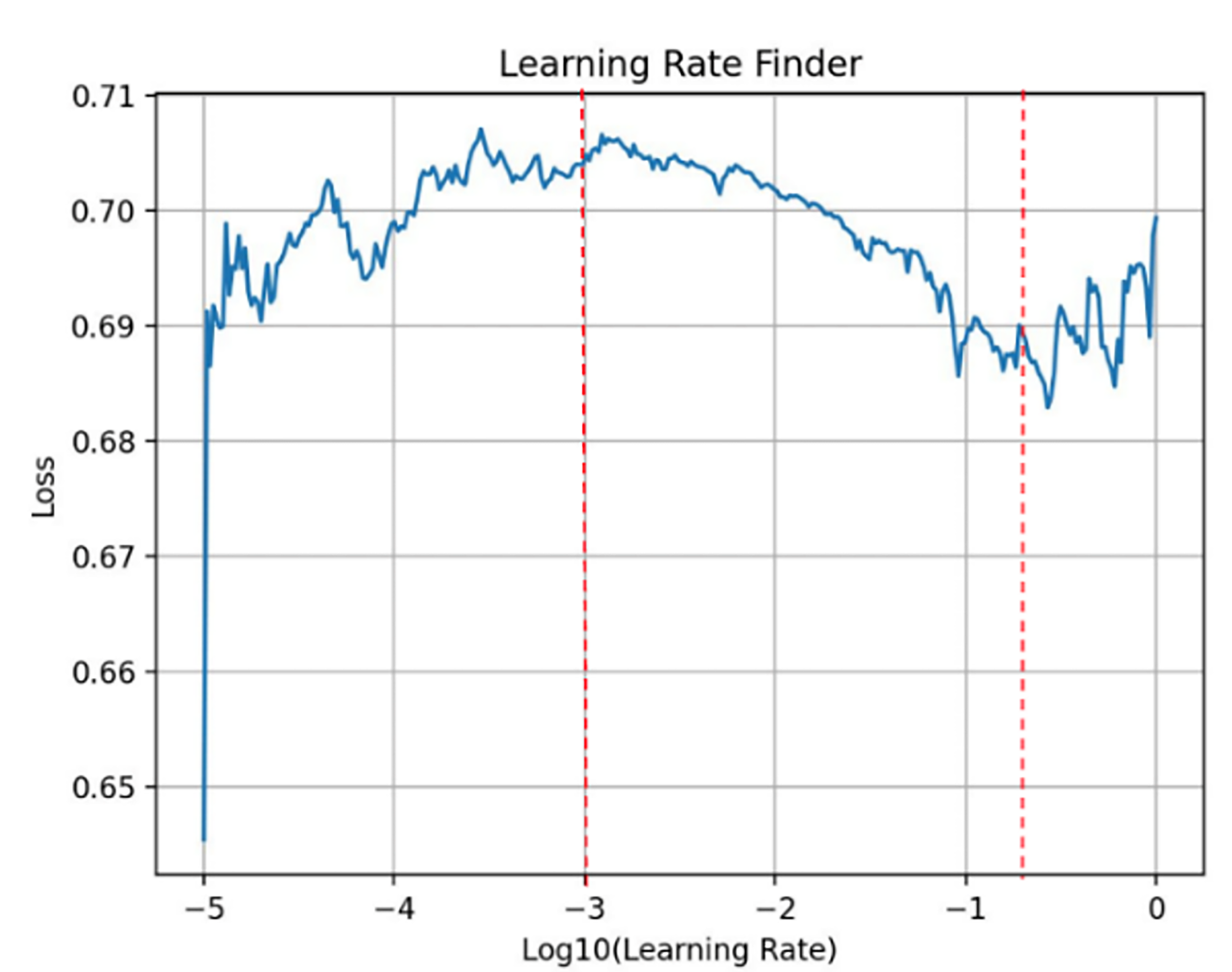
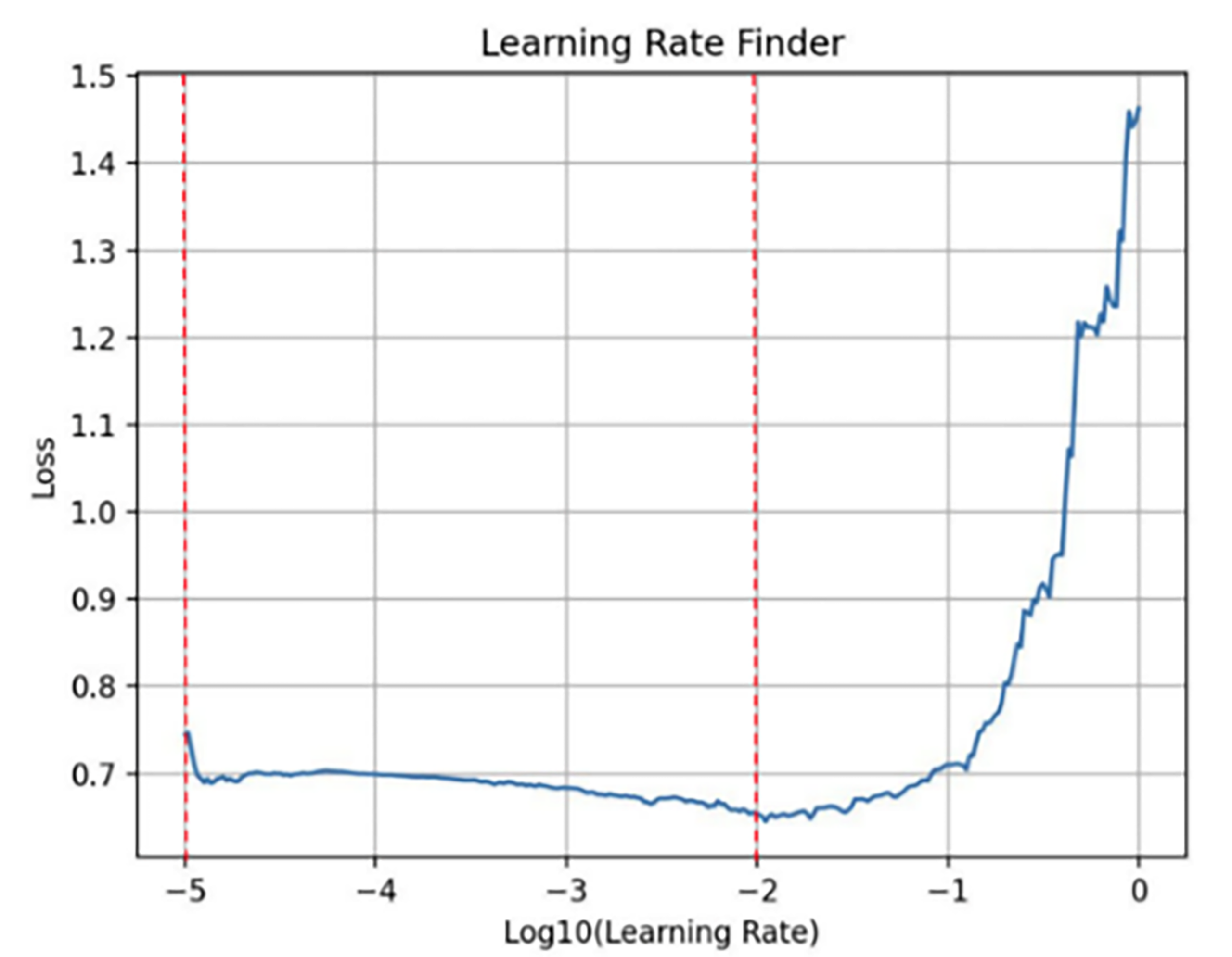
A learning rate finder was used to identify practical candidate ranges for Adam and SGD before repeated testing. In this procedure, the learning rate was gradually increased while the corresponding loss was recorded, producing a loss versus learning rate curve. The x-axis was plotted as  (Learning Rate) because the tested values were small and spanned several orders of magnitude. The resulting curves were used only to narrow the search range. The final learning rate was selected through experimental comparison of model performance.
Stochastic Gradient Descent Learning Rate Effect on Loss
ccording to Figure 2, SGD demonstrated a relatively broad candidate learning rate region, approximately between  and
 , or approximately 0.003 to 0.100. Below this range, the loss changed slowly and demonstrated unstable behavior, suggesting that learning was inefficient. Above this range, the loss began to increase, suggesting that the learning rate was too large and caused unstable updates.
Adam Learning Rate Effect on Loss
According to Figure 3, Adam demonstrated a stronger candidate learning rate region between approximately  and
 , or about 0.00001 to 0.01. Within this region, the loss decreased more effectively, while larger learning rates caused the loss to rise, indicating unstable optimization.
Experimental Testing between Adams and SGD using the Optimal Learning Rate Ranges
| Average | |||
| Learning Rate | Training Accuracy | Test Accuracy | F1 Score |
|---|---|---|---|
| 0.00001 | 0.71 | 0.68 | 0.76 |
| 0.00002 | 0.70 | 0.69 | 0.75 |
| 0.00005 | 0.72 | 0.68 | 0.73 |
| 0.00007 | 0.71 | 0.70 | 0.74 |
| 0.0001 | 0.71 | 0.73 | 0.76 |
| 0.0002 | 0.71 | 0.69 | 0.74 |
| 0.0005 | 0.70 | 0.70 | 0.76 |
| 0.001 | 0.72 | 0.71 | 0.77 |
| 0.002 | 0.71 | 0.71 | 0.76 |
| 0.003 | 0.70 | 0.71 | 0.77 |
| 0.004 | 0.73 | 0.73 | 0.77 |
| 0.005 | 0.72 | 0.71 | 0.77 |
| 0.007 | 0.70 | 0.69 | 0.75 |
| 0.009 | 0.70 | 0.69 | 0.74 |
| 0.01 | 0.69 | 0.69 | 0.74 |
| Learning Rate | Average | ||
|---|---|---|---|
| Training Accuracy | Test Accuracy | F1 Score | |
| 0.001 | 0.59 | 0.58 | 0.64 |
| 0.002 | 0.66 | 0.68 | 0.72 |
Using the code from Appendix, ranges found above by the learning rate finder, learning rates within it were experimented to determine the training accuracy, testing accuracy and F1 score provided by each. The number of hidden layers was kept constant at 2, to test for the better optimization method.
Multiple trials were conducted to reduce random errors when measuring training accuracy, test accuracy, and F1 score.
Since Adam’s optimal learning rate range was much broader (0.00001–0.01) compared to SGD’s narrower range (0.003–0.2), more learning rate values were tested for Adam during experimentation.
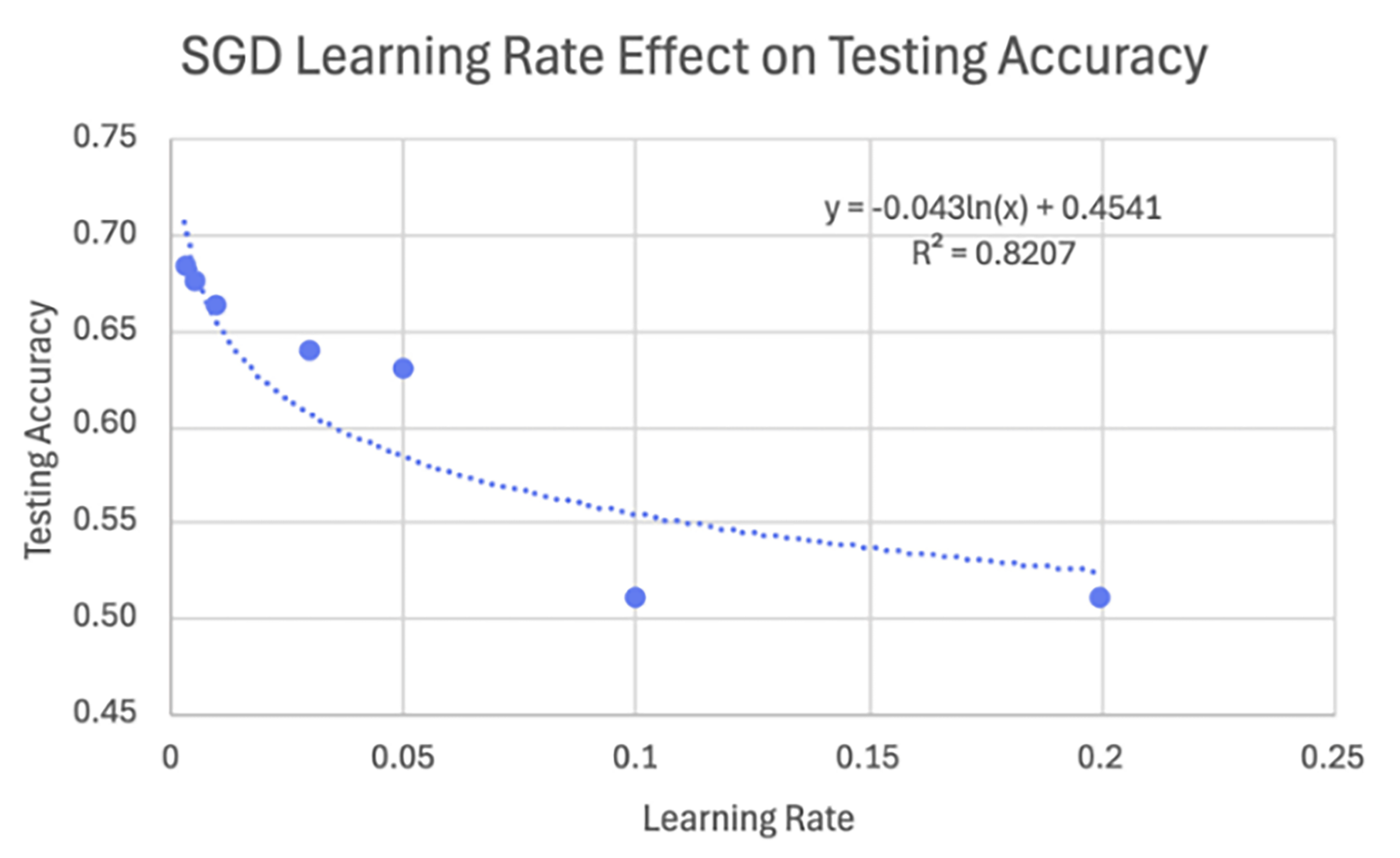
For both experiments tested below, the average results from the trials are displayed. Figure 4 displays the effect of learning rate on testing accuracy in a stochastic gradient descent model. The mathematical trend in Figure 4 displays a logarithmic relationship between the learning rate and testing accuracy, suggesting that the increase in learning rate has a diminishing effect on the test accuracy. A logarithmic regression was fitted to the experimental data, yielding:
Since the trend is logarithmic, it may seem like extrapolating the graph backwards to values lower than 0.003 will have even larger accuracies, based on the finding learning rate Figure 4, the accuracy will actually become noisier if the learning rate is decreased more, and 0.03 is the beginning of the optimal domain. However, since 0.003 was a visually fitted line, tests for 0.002 and 0.001 were conducted with the following results:
Note: The displayed results are the averages of 3 conducted trials
| Learning Rate | Average | ||
|---|---|---|---|
| Training Accuracy | Test Accuracy | F1 Score | |
| 0.003 | 0.66 | 0.68 | 0.73 |
| 0.005 | 0.67 | 0.68 | 0.72 |
| 0.01 | 0.67 | 0.66 | 0.71 |
| 0.03 | 0.67 | 0.64 | 0.69 |
| 0.05 | 0.66 | 0.63 | 0.69 |
| 0.1 | 0.51 | 0.51 | 0.21 |
| 0.2 | 0.54 | 0.51 | 0.62 |
Table 5 displays testing accuracy scores below or equal to 0.72 which was the testing accuracy score of 0.03, indicating the logarithmic trend does not continue past the optimal domain.
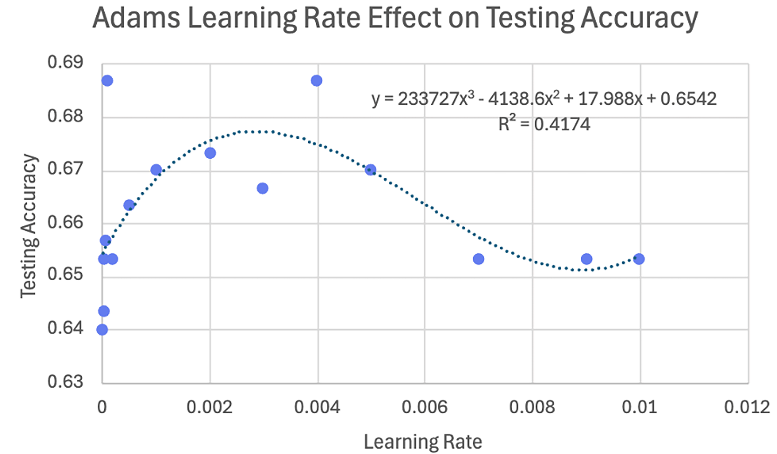
Moreover, Figure 5 illustrates the relationship between changing the learning rate on the testing accuracy of Adam model. The trend displayed in the graph is cubic trend. However, the moderate correlation of this graph is much lower compared to the SGD graph. Additionally, the R2 value is much lower than the SGD graph, indicating that there are other factors besides learning rate which significantly impacts the performance of an Adam model. Although Figure 5 displays more outliers than Figure 4, the local maximum (0.69) is higher than that of Figure 4, and the minimum value (0.64) is also higher than that of Figure 4. This suggests that the optimal learning rate for Adam would likely produce a higher testing accuracy than that of SGD. Furthermore, the cubic trend of the relationship likely represents Adam’s use of bias correction and adaptive learning rates (see equation 12). When  , the learning rate was too small, so Adam’s parameter updates were proportionally reduced, resulting in slow convergence despite adaptive moments and bias correction. Between approximately and , the loss decreased most effectively, suggesting this was the strongest candidate learning rate region. However, when
 , the loss began to increase, indicating unstable optimization cause by overly large parameter updates.
Metrics
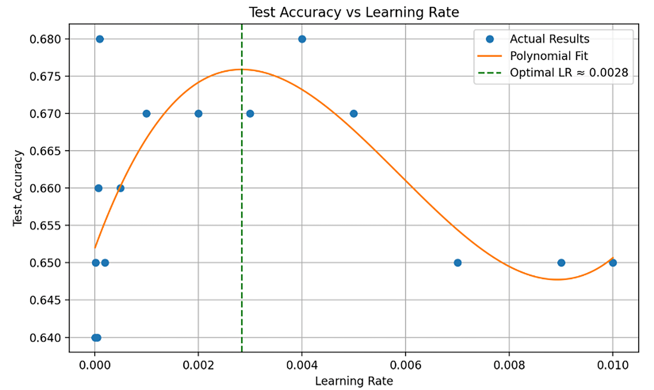
Using the test accuracy results from the Adam optimizer experiments, a cubic polynomial was fitted to model the relationship between learning rate and model performance. This smooth curve helps to visualize the general trend despite noise in the raw results. The optimal learning rate was then calculated by identifying the maximum point on this curve. As shown in the Figure 6, this optimal value was approximately 0.0028, which corresponds to the highest predicted test accuracy from the polynomial fit. This maximum was calculated using code.
Therefore, this Machine Learning Program uses Adaptive Moment Estimation (Adam) Optimization Algorithm as the optimizer because of its adaptive learning rates, suitability for noisy gradients and mini-batches, low memory requirements and being insensitive to the number of hyperparameters. This was preferred for this research question because each permutation varied in its number of swaps and of permutation size, but Adam’s adaptive updates per parameter work well with this. Adam smooths noisy gradients by using momentum so that it does not make huge jumps early in the training. Also, it converges faster than Stochastic Gradient Descent, which usually needs more epochs. Adam optimization algorithms take advantage of Momentum and RMSprop optimization algorithms22. Gradient Descent, which is the most common optimization algorithm, is much more sensitive to changes in the learning rate, has slow convergency and is difficult to navigate through noise and sparse gradients. Equations 7 to 12 follow the Adam stochastic optimization algorithm proposed by Kingma and Ba22.
Adam Algorithm:
Where is the gradient and is the loss function.
First moment estimate (mean) at time step  :
Second moment estimate (uncentered variance) at time step  :
Where is the step size for optimization, represents the decay rate for momentum and is the decay rate for squared gradients. The first momentum estimate equation (equation 8) is used to update the moving average of gradients by taking a weighted average of previous average and the current gradient. Additionally, the second moment estimate equation (equation 9) is used to update the moving average of the squared gradients.  is the Hadamard Product which is used in the second moment estimate equation for element wise multiplication. The Hadamard Product is used in the second moment estimate to allow
 to track the per-parameter variance of the gradient over time. This value is then used to scale the update step, giving each parameter its own adaptive learning rate. The use of the Hadamard Product allows the algorithm to compute the uncentered variance of each parameter’s gradient individually, rather than all together. This is significant for the algorithm to adapt its learning rate per parameter, especially in our problem where different swap sequence representations can lead to irregular and wide gradient flows.
The update of the moving average of gradients () is utilized to optimize learning in directions with consistent gradients, which is the integration of momentum. The update of the moving average of squared gradients () is the integration of RMSProp, which uses the moving average to adapt the learning rate for each parameter, scaling down updates for parameters with large gradients and up for parameters with small gradients.
The base learning rate remains constant throughout training. However, the moment estimates  and are initially biased toward zero, so they are corrected using bias-adjusted forms:
Update the model parameters using the adaptive learning rates:
Where is a small constant (around 10-8) added to the denominator to prevent the division of 0 to maintain numerical stability.  is the update parameter value at time step and is the learning rate.
Results
Table 6: Number of layers vs Testing Accuracy and F1 Score for Trials 1–5
| Layers | Trial 1 | Trial 2 | Trial 3 | Trial 4 | Trial 5 | |||||
|---|---|---|---|---|---|---|---|---|---|---|
| Test Accuracy | F1 Score | Test Accuracy | F1 Score | Test Accuracy | F1 Score | Test Accuracy | F1 Score | Test Accuracy | F1 Score | |
| 1 | 0.87 | 0.64 | 0.89 | 0.67 | 0.88 | 0.68 | 0.83 | 0.53 | 0.73 | 0.45 |
| 2 | 0.82 | 0.52 | 0.88 | 0.59 | 0.85 | 0.59 | 0.88 | 0.62 | 0.83 | 0.49 |
| 3 | 0.82 | 0.52 | 0.83 | 0.53 | 0.88 | 0.60 | 0.75 | 0.44 | 0.87 | 0.63 |
| 4 | 0.86 | 0.53 | 0.83 | 0.53 | 0.85 | 0.48 | 0.84 | 0.53 | 0.81 | 0.49 |
| 5 | 0.86 | 0.55 | 0.74 | 0.46 | 0.84 | 0.52 | 0.88 | 0.58 | 0.86 | 0.57 |
| 6 | 0.86 | 0.43 | 0.41 | 0.33 | 0.88 | 0.58 | 0.75 | 0.46 | 0.79 | 0.48 |
| 7 | 0.80 | 0.55 | 0.80 | 0.48 | 0.45 | 0.34 | 0.60 | 0.32 | 0.43 | 0.33 |
| 8 | 0.39 | 0.31 | 0.44 | 0.32 | 0.54 | 0.33 | 0.35 | 0.33 | 0.79 | 0.39 |
| 9 | 0.47 | 0.31 | 0.61 | 0.32 | 0.34 | 0.32 | 0.34 | 0.33 | 0.45 | 0.32 |
| 10 | 0.61 | 0.31 | 0.34 | 0.32 | 0.35 | 0.34 | 0.42 | 0.33 | 0.41 | 0.33 |
| Layers | Trial 6 | Trial 7 | Trial 8 | Trial 9 | Trial 10 | |||||
|---|---|---|---|---|---|---|---|---|---|---|
| Test Accuracy | F1 Score | Test Accuracy | F1 Score | Test Accuracy | F1 Score | Test Accuracy | F1 Score | Test Accuracy | F1 Score | |
| 1 | 0.78 | 0.47 | 0.85 | 0.56 | 0.89 | 0.61 | 0.87 | 0.61 | 0.84 | 0.57 |
| 2 | 0.66 | 0.40 | 0.88 | 0.61 | 0.87 | 0.64 | 0.85 | 0.53 | 0.73 | 0.49 |
| 3 | 0.71 | 0.43 | 0.89 | 0.65 | 0.89 | 0.64 | 0.84 | 0.50 | 0.88 | 0.62 |
| 4 | 0.85 | 0.58 | 0.77 | 0.47 | 0.84 | 0.54 | 0.84 | 0.53 | 0.86 | 0.51 |
| 5 | 0.89 | 0.62 | 0.81 | 0.51 | 0.84 | 0.56 | 0.86 | 0.61 | 0.67 | 0.39 |
| 6 | 0.84 | 0.54 | 0.88 | 0.57 | 0.81 | 0.53 | 0.84 | 0.55 | 0.83 | 0.53 |
| 7 | 0.81 | 0.51 | 0.74 | 0.46 | 0.83 | 0.47 | 0.84 | 0.54 | 0.87 | 0.47 |
| 8 | 0.74 | 0.43 | 0.40 | 0.32 | 0.43 | 0.33 | 0.33 | 0.33 | 0.61 | 0.32 |
| 9 | 0.61 | 0.33 | 0.35 | 0.33 | 0.42 | 0.33 | 0.34 | 0.32 | 0.33 | 0.32 |
| 10 | 0.37 | 0.33 | 0.48 | 0.33 | 0.39 | 0.36 | 0.41 | 0.33 | 0.43 | 0.32 |
| Layers | Mean | |||
|---|---|---|---|---|
| Test Accuracy | Test Accuracy Standard Dev. | F1 Score | F1 Score Standard Dev. | |
| 1 | 0.84 | 0.05 | 0.46 | 0.08 |
| 2 | 0.83 | 0.07 | 0.55 | 0.08 |
| 3 | 0.84 | 0.06 | 0.56 | 0.08 |
| 4 | 0.84 | 0.03 | 0.52 | 0.03 |
| 5 | 0.83 | 0.07 | 0.54 | 0.07 |
| 6 | 0.79 | 0.14 | 0.50 | 0.08 |
| 7 | 0.72 | 0.16 | 0.45 | 0.09 |
| 8 | 0.50 | 0.16 | 0.34 | 0.04 |
| 9 | 0.43 | 0.11 | 0.32 | 0.01 |
| 10 | 0.42 | 0.08 | 0.33 | 0.01 |
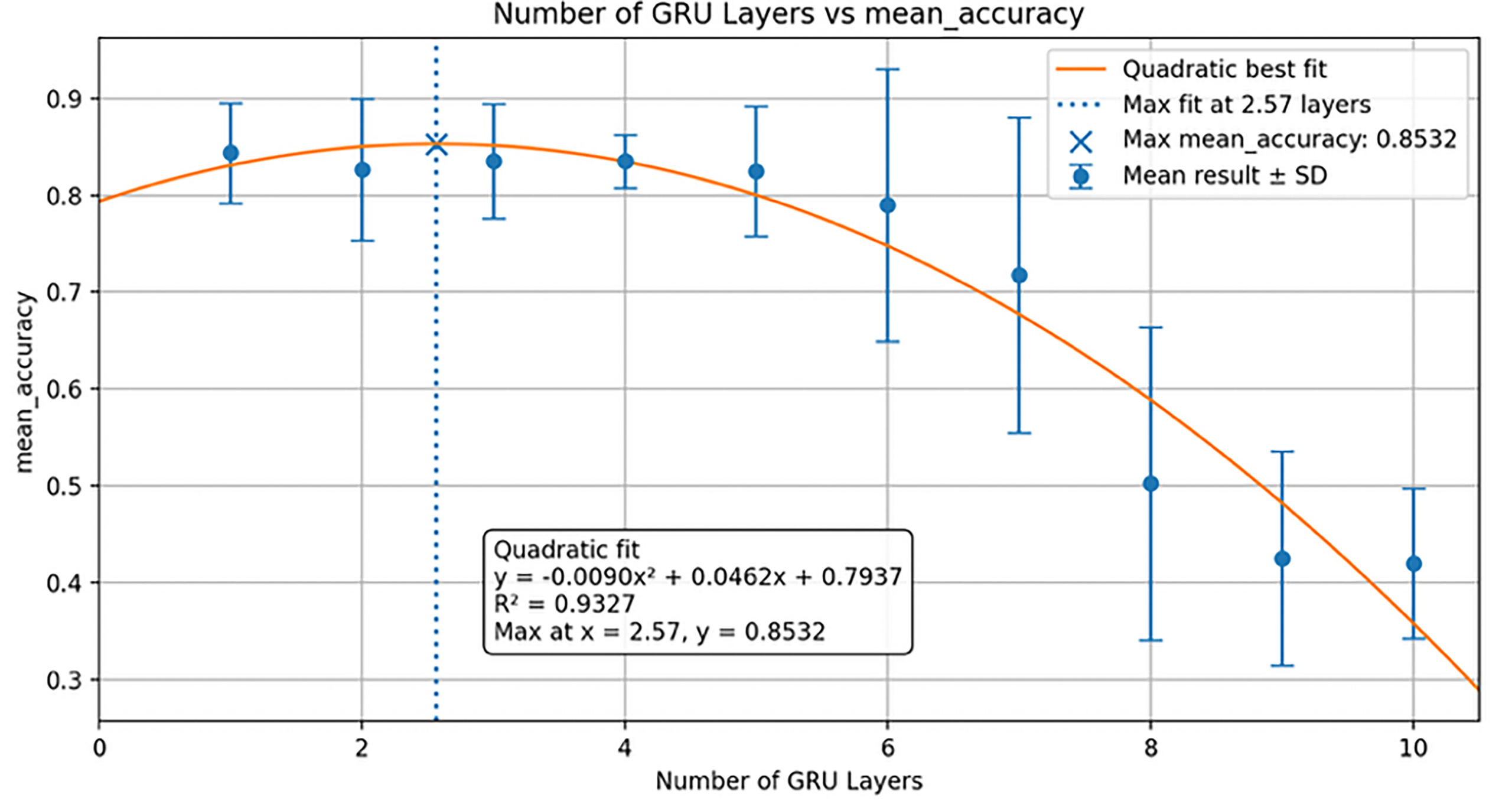
Results of Number of Layers vs the Accuracies and F1 Score of the Model, where Yellow represents outlier trials (Table 6 and 7), as determined by the Interquartile Range (IQR) Rule for when a trial’s test accuracy was below  or greater than
 :
In Figure 7, the trendline’s high  value of 0.9327 indicates a very strong correlation between the number of layers and training accuracy with a quadratic relationship. The error bars represent the test accuracy standard deviation. The trendline suggests that performance is strongest in the shallow-layer region, with the peak accuracy being 0.85 at 2.57 layers. However, because layers can only be whole numbers, the strongest observed accuracy performance occurs between 2-3 layers.
The results from Table 6, 7 and 8 demonstrate that shallow GRU configurations performed better than deeper configurations, with Layers 1, 3, and 4 achieving the highest mean test accuracy of 0.84 and Layers 2 and 5 were marginally lower with a test accuracy of 0.83. Alternatively, Layers 6 and 7 had a test accuracy of less than 0.80 and Layers 8, 9, and 10 had a test accuracy of 0.50 or lower. Additionally, F1 score is also extremely useful because the classification problem can be affected by the imbalance between complete-cycle and non-complete-cycle examples, and the F1 score was also the highest for the 3-layer model, at 0.56, followed closely by the 2-layer model at 0.55 and the 5-layer model at 0.54. Hence, suggesting that the strongest overall performance occurred around the 2–3-layer region.
Moreover, for the shallower models from 1-5 layers, the test accuracy standard deviation ranged from 0.03 to 0.07, while after 5 layers, the standard deviation increased, with the 6-layer, 7-layer, and 8-layer models having standard deviations of 0.14, 0.16, and 0.16, respectively, which are significantly greater than those of the shallow model.
| Metric | ANOVA F | df | p | η² | Kruskal-Wallis H | df | p | ε² |
| Accuracy | 29.703 | (9, 90) | <.001 | 0.748 | 61.789 | 9 | <.001 | 0.587 |
| F1 Score | 25.635 | (9, 90) | <.001 | 0.719 | 65.907 | 9 | <.001 | 0.632 |
Furthermore, 8 of the 9 outliers occurred as unusually low-test accuracy values within stronger performing layer groups. For instance, the 6-layer model had a mean test accuracy of 0.79 but Trial 2 was significantly lower at 0.41.
| L1 | L2 | L3 | L4 | L5 | L6 | L7 | L8 | L9 | L10 | |
| L1 | — | 1 | 1 | 1 | 1 | 1 | 1 | 0.003 | <.001 | <.001 |
| L2 | — | 1 | 1 | 1 | 1 | 1 | 0.015 | 0.002 | 0.002 | |
| L3 | — | 1 | 1 | 1 | 1 | 0.006 | <.001 | <.001 | ||
| L4 | — | 1 | 1 | 1 | 0.038 | 0.005 | 0.007 | |||
| L5 | — | 1 | 1 | 0.017 | 0.002 | 0.003 | ||||
| L6 | — | 1 | 0.138 | 0.022 | 0.028 | |||||
| L7 | — | 1 | 0.706 | 0.836 | ||||||
| L8 | — | 1 | 1 | |||||||
| L9 | — | 1 |
Shapiro-Wilk tests showed that the normality assumption was violated in some layer groups, especially for test accuracy, while Levene’s test indicated unequal variance for F1 score. Therefore, Kruskal-Walis H tests were used as the main statistical test to compare performance across GRU layer depths. As demonstrated in Table 9, layer depth had a statistically significant effect on both test accuracy, H(9) = 61.79, p<.001, and F1 score, H(9)=65.91, p < .001 . This indicates that model performance differed significantly across layer depths.
| L1 | L2 | L3 | L4 | L5 | L6 | L7 | L8 | L9 | L10 | |
| L1 | — | 1 | 1 | 1 | 1 | 1 | 0 | <.001 | <.001 | <.001 |
| L2 | — | 1 | 1 | 1 | 1 | 1 | 0.003 | <.001 | 0.003 | |
| L3 | — | 1 | 1 | 1 | 1 | 0.002 | <.001 | 0.002 | ||
| L4 | — | 1 | 1 | 1 | 0.042 | 0.009 | 0.048 | |||
| L5 | — | 1 | 1 | 0.006 | 0.001 | 0.007 | ||||
| L6 | — | 1 | 0.093 | 0.022 | 0.106 | |||||
| L7 | — | 1 | 0.753 | 1 | ||||||
| L8 | — | 1 | 1 | |||||||
| L9 | — | 1 |
Table 10 and 11’s Dunn’s post-hoc comparisons with Bonferroni correction demonstrated that Layers 1-7 were not statistically significantly different from one another on either test accuracy or F1 score. However, Layers 8-10 were significantly lower than most of the shallower models, especially Layers 1-6. This suggests that performance remained broadly similar across shallow-to-moderate GRU depths before declining in the deepest architectures.
Thus, the strongest performance occurred in the shallow 2–4-layer region. The 3-layer GRU achieved the highest mean F1 score, while the 4-layer GRU demonstrated the lowest standard deviation among the high accuracy models. Therefore, the results suggest that shallow GRU architectures provide the best balance between accuracy, F1 score, and stability under the tested conditions.
Discussion
Neural Network Design
The strongest observed model for learning patterns with swap-sequence data, when predicting whether the resulting permutation from a complete cycle, was a GRU-based neural network trained using the Adam optimizer with an optimized learning rate of 0.0028 and 3 hidden layers, selected for its strong and stable performance on sequential permutation data. Hence, the strongest observed GRU-based model demonstrated that sequential permutation patterns are learnable to a meaningful degree, achieving a mean test accuracy of 0.84. However, its F1 score of 0.56 indicates that prediction quality was moderate when both precision and recall where considered together, suggesting that the model captured general structure but still struggled with more complex permutation cases.
The mean F1 scores were significantly lower than the mean test accuracy scores for all layers, which was expected. This was because accuracy reflects overall correctness which can be dominated by the majority class, while F1 score is more sensitive to minority class errors through its dependence on both precision and recall23. Thus, the gap between accuracy and F1 indicates that the GRU learned the incomplete cycle class structure well, but the complete cycle class detection was weaker.
Additionally, shallow GRUs likely performed better because the task used relatively small permutations and short swap sequences, with  and
 . Hence, it may not have required the extended temporal memory that deeper recurrent architectures are designed for, because GRUs are already effective sequence models15,24. Therefore, additional recurrent layers did not provide useful extra memory for this task and instead added unnecessary parameters and optimization difficulty. Moreover, existing theory demonstrates that deeper RNNs are useful for modeling long term dependencies, implying the permutation size and swap sequence length in this experiment were not large enough for additional recurrent depth to provide a clear advantage24.
Furthermore, the GRU was compared against a majority-class baseline for a task specific context. Since 81.85% of the natural dataset consisted of non-complete cycles, a classifier that always predicted “not complete cycle” would already 81.85% accuracy, but an F1 score of 0 for complete cycles. Although, the optimal GRU’s mean test accuracy of 0.84 was only slightly higher than this baseline, it is still meaningful because the baseline accuracy was already extremely high due to the significant class imbalance. Additionally, the GRU achieved a mean F1 score of 0.56, demonstrating that it learnt a useful structure for identifying complete cycles rather than simply predicting the majority class.
Moreover, the standard deviations across layers demonstrated that performance was not equally stable across all architectures. Shallow models with fewer than 6 layers had lower standard deviations than deeper models, suggesting that increasing depth made the model less reliable. These outliers likely occur because neural network training is stochastic, with each trail involving different random initialization, data splitting, and batch ordering, which can cause occasional unusually high or low results. Deeper recurrent models may be even more sensitive to this variation because they have more parameters and are harder to optimize. Although 8 of the 9 outliers, based on IQR, occurred in models with fewer than 6 layers, this does not contradict the standard deviation trend because these shallow model outliers were isolated underperforming trails within otherwise consistently strong configurations. The remaining outlier occurred in the 10-layer model and represented an unusually high performing trial, but this was within an architecture that was already weak overall. Therefore, the outliers demonstrate that shallow GRUs rarely underperformed, but did so significantly, while deeper models were consistently less stable.
Statistical tests support the descriptive results by demonstrating that the differences among the shallow to moderate GRU models should not be overinterpreted. Although some layers had slightly higher mean accuracy or F1 scores, Layers 1-7 were not statistically distinguishable from one another. The clearer finding is that performance declined significantly in the deepest models, particularly from Layer 8 onwards. Therefore, the results suggest that increasing GRU depth did not provide reliable performance gains under the tested conditions and may have introduced optimization difficulties in deeper recurrent models.
Overall, the investigation demonstrated that GRU based neural networks can learn meaningful structure from generated swap sequences, when predicting complete-cycle structure. Descriptively, the 3-layer GRU achieved the strongest mean performance, particularly in F1 score, while the 4-layer GRU showed strong stability through its low standard deviation. However, Dunns post-hoc tests demonstrated that Layers 1-7 were not statistically distinguishable from one another. Therefore, the results do not identify a single uniquely optimal layer depth but instead suggest that shallow to moderate GRU architectures formed the strongest performance and range under the tested conditions.
This is significant because it shows that GRUs can learn useful structure from swap sequences without explicitly simulating every possible repeated application of the resulting permutation. It also suggests that increasing architectural depth does not automatically lead to better combinatorial reasoning or generalization, since performance declined from Layer 8 onward.
However, a limitation of this investigation was that the hyperparameter search was limited in scope. Although optimizer choice, learning rate, and network depth were tested, other hyperparameters such as hidden size, dropout, batch size and training schedule were not exhaustively explored. Therefore, the selected architecture should be interpreted as the strongest observed configuration within the tested settings rather than a globally optimal GRU architecture.
Future work should test whether these findings generalize to larger values of and , since longer swap sequences may require different levels of recurrent depth or memory capacity. Further research could also extend the model to predict richer structural properties, such as full cycle decompositions, rather than only binary complete-cycle labels.
Appendix
The code used during experimentation can be found on: https://github.com/Ishi17/UniMelbResearch
References
- V. Bafna, P. A. Pevzner. Sorting by Transpositions. SIAM Journal on Discrete Mathematics. Vol. 11. 1998, https://doi.org/10.1137/S089548019528280X. [↩]
- P. Diaconis, M. Shahshahani. Generating a Random Permutation with Random Transpositions. Zeitschrift fur 2 Wahrscheinlichkeitstheorie und verwandte Gebiete. Vol. 57, pg. 159 – 179. 1981, https://doi.org/10.1007/BF00535487. [↩]
- P. Velickovic, C. Blundell. Neural Algorithmic Reasoning. Patterns. Vol. 2. 2021, https://doi.org/10.1016/j.patter.2021.100273. [↩]
- K. Zhang, J. Bloom. Cyclic-permutation invariant networks for modeling periodic sequential data: application to variable star classification. In Monthly Notices of the Royal Astronomical Society. Oxford Academic. 2021, https://ml4physicalsciences.github.io/2020/files/NeurIPS_ML4PS_2020_109.pdf. [↩]
- Z. Huang, Y. Wang, C. Li, H. He. Going Deeper into Permutation-Sensitive Graph Neural Networks. International Conference on Machine Learning. 2022, https://proceedings.mlr.press/v162/huang22l/huang22l.pdf. [↩]
- M. Kimura, R. Shimizu, Y. Hirakawa, R. Goto, Y. Saito. On permutation-invariant neural networks. Arxiv. 2024, https://doi.org/10.48550/arXiv.2403.17410 [↩]
- A. Paszke, S. Gross, R. Massa, A. Lerer, J. Bradbury, G. Chanan, T. Killeen, Z. Lin, N. Gimelshein, L. Antiga, A. Demaison, A. Kopf, E. Yang, Z. DeVito, M. Raison, A. Tejani, S. Chilamkurthy, B. Steiner, L. Fang, J. Bai, S. Chintala. PyTorch: An Imperative Style, High-Performance Deep Learning Library. 33rd Conference on Neural Information Processing Systems. Vol. 32. pg. 8026 – 8037. 2019, https://dl.acm.org/doi/10.1145/3814779. [↩]
- I. Goodfellow, Y. Bengio, A. Courville. Deep Learning. The MIT Press. 2016. [↩]
- W. H. Saputra, R. Nariswari, M. Owen. On the recurrent neural network model with robust expectation-based loss function in economic data forecasting. MethodsX. Vol. 15. 2025, 10.1016/j.mex.2025.103718. [↩]
- S. Hochreiter, J. Schmidhuber. Long Short-Term Memory. Neural Computation. Vol. 9, pg: 1735-1780. 1997, 10.1162/neco.1997.9.8.1735. [↩]
- K. Cho, B. V. Merrienboer, C. Gulcehre, D. Bahdanau, F. Bougares, H. Schwenk, Y. Bengio. Learning Phrase Representations using RNN Encoder-Decoder for Statistical Machine Translation. Proceedings of the 2014 Conference on Empirical Methods in Natural Language Processing. 2014, 10.3115/v1/D14-1179. [↩] [↩]
- Y. Bengio, P. Simard, P. Frasconi. Learning long-term dependencies with gradient descent is difficult. IEEE Transactions on Neural Networks. Vol. 5, pg. 157–166. 1994, 10.1109/72.279181. [↩]
- T. Lee, V. P. Singh. Deep learning: Long short-term memory in hydrological time series. Handbook of Hydrologinformatics Impacts. Elsevier. pg. 49–67. 2023, https://doi.org/10.1016/B978-0-12- 821961-4.00022-1. [↩]
- S. Yang, X. Yu, Y. Zhou. LSTM and GRU Neural Network Performance Comparison Study: Taking Yelp Review Dataset as an Example. 2020 International Workshop on Electronic Communication and Artificial Intelligence. 2020, 10.1109/IWECAI50956.2020.00027. [↩]
- J. Chung, C. Gulcehre, K. Cho, Y. Bengio. Empirical Evaluation of Gated Recurrent Neural Networks on Sequence Modeling. NIPS 2014 Deep Learning and Representation Learning Workshop. 2014, https://doi.org/10.48550/arXiv.1412.3555. [↩] [↩]
- C. M. Bishop. Pattern Recognition and Machine Learning. Springer. 2006. [↩]
- D. Cemernek, S. Siddiqi, R. Kern. Effects of class Imbalance Countermeasures on Interpretability. IEEE Access. Vol. 12. 2024, 10.1109/ACCESS.2024.3381536. [↩]
- Amazon Web Services. What is hyperparameter tuning? – hyperparameter tuning methods explained – AWS. Amazon Web Services, Inc. 2024, https://aws.amazon.com/whatis/hyperparameter-tuning/. [↩]
- N. Srivastava, G. Hinton, A. Krizhevsky, I. Sutskever, R. Salakhutdinov. Dropout: A Simple Way to Prevent Neural Networks from Overfitting. Journal of Machine Learning Research. Vol. 15, pg. 1929–1958. 2014, https://dl.acm.org/doi/10.5555/2627435.2670313. [↩]
- A. C. Wilson, R. Roelofs, M. Stern, N. Srebro, B. Recht. The Marginal Value of Adaptive Gradient Methods in Machine Learning. Advances in Neural Information Processing Systems. 2017, https://doi.org/10.48550/arXiv.1705.08292. [↩]
- M. Mishra. The learning rate: a hyperparameter that matters. Medium. 2023, https://mohitmishra786687.medium.com/the-learning-rate-a-hyperparameter-that-mattersb2f3b68324ab. [↩]
- D. P. Kingma, B. Jimmy. Adam: A Method for Stochastic Optimization. 3rd International Conference for Learning Representations. 2017, https://doi.org/10.48550/arXiv.1412.6980. [↩] [↩]
- H. N. Gercek. Limitations of Evaluation Metrics Under Class Imbalance. Alto University. 2026, https://urn.fi/URN:NBN:fife202504262412. [↩]
- Y. Levine, O. Shashua. Benefits of Depth for Long-Term Memory of Recurrent Networks. ICLR 2018 Conference. 2018, https://openreview.net/pdf?id=HJ3d2Ax0-. [↩] [↩]