Family history, lifestyle, and the prevalence of hypertension

March 26, 2026

Abstract

Hypertension is one of the most significant risk factors contributing to cardiovascular diseases, and family history is a useful screening tool in hypertension interventions. However, systematic evaluation of the effect of family history and its interactions with lifestyle on hypertension is scarce. Using data from the 2018 Fifth Chronic Disease Monitoring Survey in Shandong Province, we estimate this effect using both propensity score matching and a standard Logistic regression model. We find consistent evidence for first-degree family history as an important risk factor for hypertension in both models, whilst the effect of second-degree family history is inconclusive. We further compare results of the two models with respect to implied assumptions, core concepts, and sample sizes. We conclude that maintaining a healthy lifestyle, especially controlling body weight, is essential for people both with and without family history. In particular, weight control can lead to a greater reduction in risk for people with more first-degree relatives with family history. We contribute to the literature by providing an elaborate analysis of the effect of family history and its interactions with lifestyle. This study can also be utilized to identify the population defined by risk factors of family history who might disproportionately benefit from lifestyle interventions, which is directly relevant to precision prevention and clinical applications.

Keywords: Family History; Lifestyle; Hypertension; Propensity Score Matching; Logistic Regression Model

Introduction

As a chronic noncommunicable disease, hypertension is one of the most preventable risk factors for cardiovascular disease and all-cause mortality¹^,². It continues to be a significant public health concern and has affected over one billion people all over the world³^,⁴. Since 1990, the number of people with hypertension has doubled worldwide⁵.

It is widely accepted that hypertension is caused by multifactorial genetic, environmental, and physiological factors⁶^,⁷^,⁸. Specifically, family history is a useful screening tool in hypertension interventions. However, systematic evaluation of first-degree versus second-degree family history, and the interactions of family history (FH) with modifiable lifestyle on hypertension is scarce. Furthermore, previous studies estimating the associations between various risk factors and the distribution of hypertension risk have primarily used the Logistic regression model⁹^,¹⁰^,¹¹, which adjusts for confounders within the statistical model. In contrast, propensity score matching (PSM) addresses the same issue by improving the comparability of groups prior to outcome analysis, offering a design-based advantage¹².

The aim of this study is to explore the role of FH with different degrees of familial relation and its possible interactions with lifestyle factors (including body mass index, central obesity, drinking, smoking, and physical exercise) in the distribution of hypertension risk. The data we use comprises 8,116 participants enrolled in the Fifth Chronic Disease Monitoring Survey in Shandong Province in 2018. The survey data contains detailed information on family history of hypertension, including paternal, maternal, sibling, grandfather, and grandmother sources, allowing us to provide an in-depth analysis of the effect of FH on hypertension prevalence.

We additionally employ propensity score matchingin this study to enhance comparability between participants with and without FH, besides the generally adopted Logistic regression model. It is important to note that neither propensity score matching nor Logistic regression model can address the omitted-variable bias caused by unobserved confounders, which should be a focus for correction in future research that utilizes more advanced causal inference techniques.

Our results indicate that the association of FH and the distribution of hypertension risk is statistically significant in both models. We find that the effect of first-degree FH is consistently significant for the prevalence of hypertension, whilst the effect of the second-degree FH is insignificant and inconclusive. We then estimate the effects of paternal/maternal/sibling sources and the number of first-degree relatives with FH, respectively and the results remain undisturbed. We further explore the interactions of first-degree FH and lifestyle, and find that weight control is more essential for individuals with more first-degree relatives with FH.

We hence contribute to the literature by providing an elaborate analysis of the effect of family history and its interactions with lifestyle, and add to the strand of literature on precision prevention as well¹³^,¹⁴. Although family history of hypertension (FH) might reflect not only genetic but lifestyle factors¹⁵^,¹⁶, it is still a very important proxy variable for genetics¹⁷. Therefore, this study also sheds light on the impact of genetics on hypertension prevalence¹⁸^,¹⁹.

Methods

Data

We obtained the data from the fifth chronic disease monitoring survey conducted by the Shandong Center for Disease Control and Prevention in 2018. The primary goal for the continuous monitoring is to analyze the prevalence of chronic noncommunicable diseases in different areas and among people across the province of Shandong, thereby providing the basic data for formulating and evaluating the related public health policies.

The monitoring points comprise 14 districts: 6 urban and 8 rural. The monitoring data include the questionnaire at both the family and individual levels, body measurements, and biochemical tests. The monitoring sample comprises 8,492 adult participants, selected using a multi-stage cluster random sampling method to ensure it is representative of the whole province. The final study sample contains 8,116 observations after excluding participants with missing values.

The monitoring variables fall into three categories: continuous, categorical, and dummy. We convert all continuous variables into categorical or dummy ones to enhance interpretability and clinical relevance. This allows findings to be directly linked to established clinical thresholds, making results actionable for risk communication and policy. This approach also facilitates the identification of nonlinear relationships and simplifies the presentation of subgroup or interaction effects. However, this comes with notable statistical trade-offs like discarding within-group variation and reducing statistical power. Despite these limitations, categorization is often a pragmatic compromise to bridge complex statistical models with real-world decision-making. Furthermore, categorization is also advantageous for propensity score matching as it is not possible to find perfect matches for continuous variables²⁰.

Hypertension and family history (FH)

Hypertension

We define a participant as suffering from hypertension when one of the three conditions is met and 0 otherwise²¹: (1) Systolic blood pressure (SBP) $\ge$ 140mmHg; (2) Diastolic blood pressure (DBP) $\ge$ 90mmHg; (3) The participant has ever been diagnosed with hypertension in the county-level hospital or higher.

Family history

Risk factors for hypertension can be divided into two categories: non-modifiable and modifiable. The former includes factors that cannot be changed, such as gender, age, and genetics, whilst the latter comprises factors that can be improved, such as lifestyle factors, diet, drinking, and smoking.In our dataset, we can observe detailed family history information that reflects each participant’s genetics and lifestyle. This information was obtained by asking participants whether their biological father, mother, siblings, grandfather, or grandmother had been diagnosed with hypertension by a doctor.

The relatives can be categorized as first- and second-degree ones. The former ones share about 50% of their genes with the participant, and they are the closest blood relatives (parents, siblings, and children). The latter share about 25% of their genes, and they are still blood relatives (grandparents, aunts & uncles, nieces & nephews, and half-siblings), but the genetic link is not as direct as the first-degree ones. The survey data allows us to identify whether the hypertension family history is classified as the first-degree FH (paternal, maternal, and sibling sources) or the second-degree FH (grandfather and grandmother sources), or both.

Figure 1 demonstrates the percentage of hypertension among different FH subgroups. Panel (A) shows that the hypertension rate is higher for participants with FH than for those without FH. Panel (B) further presents that the percentage for participants with first-degree FH is higher than with second-degree FH. We then decompose the first-degree FH into paternal, maternal, and sibling sources and the second-degree FH into grandfather and grandmother sources, respectively. The results in Panel (C) are consistent with Panel (B). As both Panel (B) and (C) indicate that the percentage of hypertension for first-degree FH is much higher than the one for second-degree FH, we plot the percentage for the number of first-degree relatives with FH among paternal, maternal, and sibling sources in Panel (D). It is clear that the percentage is increasing monotonically with the number of first-degree relatives with FH.

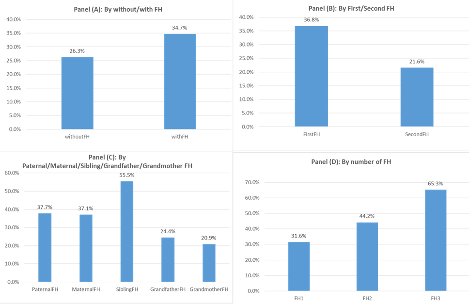
**Figure 1 | Percentage of hypertension among family history groups**
***Notes:*** This figure presents the percentage of hypertension among different family history groups. Sample are divided by with and without FH in Panel (A), by first- and second- degree FH in Panel (B), by paternal, maternal, sibling, grandfather, and grandmother sources in Panel (C), and by 1, 2, and 3 relatives with FH among paternal, maternal, and sibling sources denoted by FH1, FH2, and FH3 respectively in Panel (D).

Covariates

Individual demographic and other basic information

(1) Gender (1 for males and 0 for females).

(2) Age (three categories of Age 18-44, Age 45-59, and Age 60 and over).

(3) Nationality (1 for Han and 0 otherwise).

(4) Urban (1 for urban and 0 for rural).

(5) Insurance (1 for holding medical insurance and 0 otherwise).

(6) Education (three categories of Elementary school or lower, High school, including junior and senior, and Higher Education).

(7) Marital status (three categories of Single, Married including cohabitation, and Divorced including widowed or separated).

Lifestyle variables

(1) Body Mass Index (three categories of Normal with BMI less than 24, Overweight with BMI between [24,28), and obesity with BMI equal to or over 28). The low group with BMI less than 18.5 is merged into the Normal group for convenience.

(2) Central Obesity (equal to 1 when the waist circumference is $\ge$ 85cm for males and $\ge$ 80cm for females, and 0 otherwise)²².

(3) Drinking (three categories of never drink, drink but not every week, and drink every week during the last 12 months).

(4) Smoking (three categories of never smoke, smoke before but not anymore, and smoke now).

(5) Exercise taking (three categories of taking intensive exercise, taking moderate exercise, and never taking exercise).

Other chronic noncommunicable diseases

(1) Coronary Heart Disease (CHD, 1 for suffering and 0 otherwise).

(2) Stroke (1 for suffering and 0 otherwise).

(3) Renal Diseases (1 for suffering and 0 otherwise).

(4) Diabetes (1 for suffering and 0 otherwise).

Table 6 summarizes the covariates for participants with and without FH in columns (1) and (2), respectively. Column (3) presents the p-values from Pearson’s chi-squared tests comparing the two groups across all these covariates. It indicates that the two groups are statistically different except for nationality, urban, marital status, some lifestyle variables, and chronic diseases. This justifies employing propensity score matching to create more comparable groups for analyzing the effect of family history on hypertension.

Methods and research hypotheses

We employ both propensity score matching and a standard multivariable Logistic regression model to estimate the association between family history and hypertension. The model specifications for these two methodologies are provided in Appendix A and B, respectively. While they share a common statistical foundation as the Logistic regression model is often used to estimate the propensity score, they serve different primary purposes and provide complementary analytical strengths. The Logistic regression model provides a direct and efficient estimate of the association, expressed as an odds ratio, accounting for all specified covariates in a single model. In contrast, the primary goal of propensity score matching is to make participants with and without FH more directly comparable, thereby reducing estimation bias. Based on the existing literature and our analytical framework, this study aims to test the following hypotheses regarding the relationship between family history and hypertension prevalence.

H1: Participants with FH have a significantly higher risk of developing hypertension themselves. Specifically, participants with first-degree FH (paternal/maternal/sibling sources) will have a higher risk of hypertension than those with only a second-degree FH. Furthermore, we hypothesize that the hypertension risk will escalate progressively with the number of first-degree relatives with FH increasing.

H2: The magnitude of the odds for hypertension will escalate with the level of the underlying risk associated with the interaction between FH (first-degree) and lifestyle factors (including body mass index, central obesity, drinking, smoking, and physical exercise) increasing. Furthermore, the multiplicative interaction effect is statistically significant.

H3: The magnitude of the odds for hypertension will escalate with the level of the underlying risk associated with the interaction between the number of first-degree relatives with FH and lifestyle factors (including body mass index, central obesity, drinking, smoking, and physical exercise) increasing. Furthermore, the multiplicative interaction effect is statistically significant.

H4: Overweight and obesity increase hypertension risk within all family history groups (paternal/maternal/sibling sources and number of first-degree relatives with FH). Furthermore, compared to the reference group with normal BMI, the odds ratio for hypertension will be significantly elevated from overweight to obesity.

Results

We present the results using propensity score matching and the Logistic regression model in this section. We conduct the comparative analysis between them and estimate the odds ratios for overweight and obesity relative to normal BMI for hypertension by FH category in this section.

Results from propensity score matching

Data balancing

We adopt five matching methods of nearest-neighbor, caliper, nearest-neighbor within caliper, kernel, and local linear regression to estimate the effect of family history on the prevalence of hypertension. The rationale both for the nearest-neighbor and caliper matching is to find the “nearest neighbors” among participants without FH for each participant with FH and to calculate the arithmetic mean for hypertension. As 1:n matching can increase precision over 1:1 matching²³, and specifically 1:4 matching can minimize the mean squared error²⁴, we adopt 1:4 nearest-neighbor matching in this study. For kernel and local linear regression matching, the idea is to calculate the weighted mean²⁵ – the difference only lies in that the former uses a kernel function to calculate the weight whilst the latter employs local linear regression.

Among the five matching algorithms employed, nearest-neighbor matching within the caliper is specified as our primary analytical method. This choice is motivated by its established balance between bias reduction and efficiency. The caliper prevents poor matches by imposing a maximum allowable distance on the propensity score, thereby prioritizing the quality of covariate balance. Meanwhile, the nearest-neighbor rule within the caliper retains the maximum number of high-quality matches possible.

A prerequisite for matching is that the propensity scores for groups with and without FH have common supports as depicted in Figure A1. After deleting observations out of common support, the number of observations (N) changes from 8,116 for the unmatched sample to 8,098 for the matched sample, as shown in Table A1. Therefore, the scope of common support is large enough to allow unbiased estimation. Table A1 also presents the matched sample summary statistics for participants with and without FH in Columns (4) and (5), respectively, and the p-values based on Pearson’s chi-squared test are demonstrated in Column (6). It turns out that most variables are statistically indistinguishable between the two groups after matching. Furthermore, we depict the standardized % bias for the covariates both for the unmatched and matched samples in Figure 2. The standardized bias is defined by

$\frac{\left|\overline{c_{\text{withFH}}} - \overline{c_{\text{withoutFH}}}\right|}{\sqrt{\frac{s_{c,\text{withFH}}^2 + s_{c,\text{withoutFH}}^2}{2}}}$

where $\overline{c_{\text{withFH}}}$ and $\overline{c_{\text{withoutFH}}}$ denote the means, ${s_{c,\text{withFH}}^2$ and $s_{c,\text{withoutFH}}^2}{2}}}$ denote the variances of the groups with and without FH, respectively. It is generally accepted that a standardized bias of less than 10% for most covariates can indicate data balancing. Figure 2 shows that most standardized % biases decrease sharply after matching, and all biases in the matched sample are lower than 10%, thereby demonstrating data balancing.

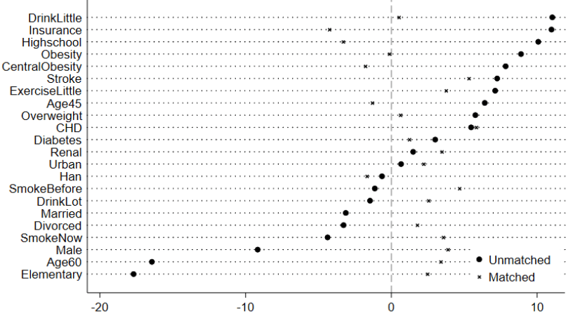
**Figure 2 | Standardized % bias across covariates before and after matching**
***Notes:*** This figure presents the standardized % bias for the covariates both in the unmatched and matched samples. The definitions of the variables are presented in the section of Methods. The 1:4 nearest-neighbor matching within the caliper (0.05) is performed.

Matching estimations

Table 1 demonstrates the estimates from the five matching methods. It shows that the mean of hypertension for the group with FH is 0.346, whilst the means for groups without FH fall in the scope of [0.242, 0.253] depending on the matching method used. According to our preferred method of nearest-neighbor within the caliper, the difference of hypertension probability between the groups with and without FH is 0.103, indicating that the probability of participants with FH suffering from hypertension is higher than that of participants without FH by 10.3%.

The other four methods serve as sensitivity analyses to confirm that our findings are not contingent on the specific algorithmic choice. All the results by these five methods confirm Hypothesis 1 that participants with FH have a significantly higher risk of developing hypertension themselves (H1).

	(1)	(2)	(3)	(4)	(5)
With FH	0.346	0.346	0.346	0.346	0.346
Without FH	0.242	0.250	0.242	0.250	0.253
Difference	0.104	0.095	0.103	0.096	0.093
T-stat	9.04	9.08	9.00	9.11	7.61
Matching approaches	NN	Caliper	NN & Caliper	Kernel	Local Linear

Table 1 | Estimations by 5 matching approaches

Notes: The matching methods listed from Column (1) to Column (5) refer to the nearest-neighbor (1:4), caliper (0.05), the 1:4 nearest-neighbor within the caliper (0.05), kernel, and local linear regression, respectively. Specifically, the caliper is calculated as 0.0996, and the algorithm can be found in Appendix A. We prioritize match precision over sample size by lowering the scope of the calculated caliper to 0.05. That means we match observations that differ within the 5% range of the propensity score. We also re-estimate with a caliper of 0.0996, and the results do not change fundamentally.

Results from Logistic regression model

Baseline estimations

We demonstrate the odds ratios and the corresponding confidence intervals for FH categories in 4 models after adjusting for individual basic information, lifestyle, and other chronic diseases in Table 2. Model 1 indicates that the odds ratio for participants with FH is 1.733 (95% CI: 1.552, 1.935) relative to participants without FH. We then decompose FH into first- and second-degree sources in Model 2 and further into paternal, maternal, siblings, grandfather, and grandmother sources in Model 3. The odds ratios for participants with first- and second-degree FH are 1.707 (95% CI: 1.531, 1.902) and 1.045 (95% CI: 0.848, 1.286), respectively as shown in Model 2. Model 3 confirms the results.

As both Model 2 and Model 3 demonstrate that the odds ratio of first-degree FH is significant, whilst the second-degree FH is not, we now particularly explore the odds ratios of the number of first-degree relatives with FH in Model 4. This indicates that the odds ratio increases from 1.453 (95% CI: 1.286, 1.642) to 3.985 (95% CI: 2.847, 5.576) as the number of first-degree FH relatives increases from 1 to 3 among paternal, maternal, and sibling sources. Therefore, Hypothesis 1 is confirmed by all four models in Table 2. Furthermore, we utilize both the Pseudo-R²and the percentage correctly predicted to measure the goodness-of-fit of different models. Table 2 indicates that the Pseudo-R²ranges from 0.178 to 0.183, and the percentage correctly predicted ranges from 74.21% to 74.95%. The goodness-of-fit of Model 4 is the highest among the four models for both measures.

	(1)	(2)	(3)	(4)	(5)	(6)	(7)	(8)
	Model 1		Model 2		Model 3		Model 4
	OR	CI	OR	CI	OR	CI	OR	CI
Without FH	1.00
With FH	1.733	[1.552,1.935]
Without FH			1.00
First-degree FH			1.707	[1.531,1.902]
Second-degree FH			1.045	[0.848,1.286]
Without FH					1.00
Paternal FH					1.49	[1.283,1.731]
Maternal FH					1.466	[1.282,1.678]
Sibling FH					1.621	[1.331,1.974]
Grandfather FH					0.955	[0.698,1.305]
Grandmother FH					0.949	[0.712,1.265]
Without First-degree FH							1.00
Number = 1							1.453	[1.286,1.642]
Number = 2							2.214	[1.836,2.670]
Number = 3							3.985	[2.847,5.576]
Covariates	Yes		Yes		Yes		Yes
Pseudo-R²	0.178		0.179		0.179		0.183
Correctly predicted	74.37%		74.21%		74.87%		74.95%

Table 2 | Effects of FH on hypertension

Notes: This table presents the odds ratios and corresponding confidence intervals for FH categories across 4 models, adjusted by the covariates, including the participants’ basic information, lifestyle, and chronic diseases listed in the section of Methods. The odd columns report the odds ratios, whilst the even columns give the confidence intervals associated with each odds ratio.

Multiplicative interactions of FH and lifestyle

In this section we interact first-degree FH with lifestyle including the BMI (Normal, Overweight, and Obesity), Drinking (Drink never, Drink not each week, and Drink each week), Smoking (Smoke never, Smoke before, and Smoke now), and exercise taking (Intensive, Moderate, and Never) to explore the multiplicative interactions for hypertension in Panels (A)’ (B)’ (C), and (D) of Table 3, respectively.

As hypothesized by H2, the odds ratio is increasing monotonically with the risk factors for the interactions of the first-degree FH with BMI categories in Panel (A). Relative to the participants with the lowest risk of without first-degree FH and with normal BMI, the odds ratio is 4.932 (95% CI: 3.925,6.198) for the riskiest group of participants with both first-degree FH and obesity. In contrast, for the other lifestyle of drinking, smoking, and exercise taking, there does not exist such a monotonously increasing trend.

We then perform a likelihood ratio test (LRT) to inspect whether the multiplicative interactions are statistically significant, with the test statistics reported in Column (5) and the corresponding p-values in Column (6). As all p-values are greater than 0.05, we cannot reject the null hypothesis that the full model specification with interactions provides statistically insignificant results compared with the reduced model without interactions. That is, our data do not support the existence of multiplicative interaction effects for first-degree FH and the lifestyle hypothesized by H2 at the conventional 5% significance level.

	(1)	(2)	(3)	(4)	(5)	(6)
	Without first-degree FH		With first-degree FH		LRT	p-value
	OR	CI	OR	CI	LRT	p-value
	Panel (A)
Normal_BMI	1.00		1.633	[1.336,1.996]	3.12	0.210
Overweight	1.479	[1.227,1.783]	2.818	[2.321,3.420]
Obesity	3.223	[2.596,4.000]	4.932	[3.925,6.198]
	Panel (B)
Drink Never	1.00		1.789	[1.556,2.056]	1.07	0.586
Drink not each week	0.991	[0.800,1.227]	1.539	[1.556,2.056]
Drink each week	1.358	[1.128,1.636]	2.223	[1.807,2.734]
	Panel (C)
Smoke Never	1.00		1.797	[1.579,2.044]	5.02	0.081
Smoke Before	1.183	[0.905,1.547]	1.351	[0.982,1.858]
Smoke Now	1.04	[0.861,1.256]	1.744	[1.406,2.164]
	Panel (D)
Intensive Exercise	1.00		1.955	[1.225,3.120]	1.47	0.480
Moderate Exercise	1.002	[0.693,1.449]	1.918	[1.320,2.785]
No Exercise	1.149	[0.820,1.608]	1.891	[1.346,2.658]

Table 3 | Multiplicative interactions of first-degree FH and lifestyle

Notes: This table presents the multiplicative interactions of the first-degree FH with lifestyle of BMI, Drinking, Smoking, and Exercise taking in Panels (A)’ (B)’ (C), and (D), respectively. Columns (1) and (3) provide the odds ratios, and the corresponding confidence intervals are given in Columns (2) and (4). All regressions across the four panels are adjusted for covariates, including participants’ basic information, lifestyle, and chronic diseases listed in the section of Methods. Columns (5) and (6) give the likelyhood-ratio test statistics and their corresponding p-values, respectively.

We further interact the number of first-degree relatives with FH among paternal, maternal, and sibling sources with the lifestyle (BMI, Drinking, Smoking, and Exercise taking) in Table 4. The results confirm hypothesis H3 by demonstrating that the ratio escalates with the level of the underlying risk associated with the interaction between the number of first-degree relatives with FH and BMI categories. Specifically, the odds ratio for participants with obesity and 3 first-degree relatives with FH (serious family history) is 8.587 (95% CI: 4.565,16.151) relative to participants without first-degree FH and with normal BMI. Again, the monotonously escalating trend is not salient for the interaction of the number of first-degree relatives with FH with the other lifestyle factors of drinking, smoking, and exercise taking. Furthermore, all LRT test statistics are statistically insignificant as shown by the p-values in Table 4.

	(1)	(2)	(3)	(4)	(5)	(6)	(7)	(8)	(9)	(10)
	Number = 0		Number = 1		Number = 2		Number = 3		LRT	p-value
	OR	CI	OR	CI	OR	CI	OR	CI	LRT	p-value
	Panel (A)
Normal_BMI	1		1.42	[1.127,1.789]	2.118	[1.482,3.029]	2.986	[1.594,5.594]	8.54	0.2009
Overweight	1.506	[1.248,1.817]	2.355	[1.902,2.914]	4.02	[2.981,5.422]	9.551	[5.555,16.423]
Obesity	3.247	[2.612,4.037]	4.356	[3.383,5.609]	5.778	[4.071,8.201]	8.587	[4.565,16.151]
	Panel (B)
Drink Never	1		1.512	[1.290,1.771]	2.329	[1.837,2.954]	4.647	[2.982,7.240]	4.37	0.6263
Drink not each week	0.989	[0.798,1.225]	1.359	[1.045,1.769]	1.562	[1.004,2.430]	2.561	[1.214,5.402]
Drink each week	1.342	[1.113,1.618]	1.834	[1.443,2.330]	3.279	[2.262,4.754]	5.161	[2.477,10.752]
	Panel (C)
Smoke Never	1		1.562	[1.350,1.807]	2.189	[1.759,2.725]	4.515	[3.028,6.730]	8.65	0.1943
Smoke Before	1.143	[0.872,1.499]	1.21	[0.827,1.771]	1.531	[0.835,2.808]	3.246	[0.903,11.668]
Smoke Now	1.032	[0.854,1.247]	1.343	[1.044,1.728]	3.015	[2.015,4.511]	3.125	[1.497,6.528]
	Panel (D)
Intensive Exercise	1		1.532	[0.890,2.637]	3.175	[1.563,6.451]	5.643	[1.353,23.534]	6.15	0.4065
Moderate Exercise	1.016	[0.702,1.471]	1.575	[1.060,2.342]	3.045	[1.833,5.056]	2.628	[1.190,5.801]
No Exercise	1.158	[0.826,1.623]	1.656	[1.170,2.343]	2.314	[1.576,3.397]	5.182	[3.099,8.663]

Table 4 | Multiplicative interactions of number and lifestyle

Notes: This table presents the multiplicative interactions of the number of first-degree relatives with FH among paternal, maternal, and sibling sources with the lifestyle of BMI, Drinking, Smoking, and Exercise in Panels (A)’ (B)’ (C), and (D), respectively. Columns (1)’ (3)’ (5), and (7) provide the odds ratios and the corresponding confidence intervals are given in Columns (2)’ (4)’ (6), and (8). All regressions across the four panels are adjusted for covariates, including participants’ basic information, lifestyle, and chronic diseases listed in the section of Methods. Columns (9) and (10) give the likelyhood-ratio test statistics and their corresponding p-values. Number denotes the number of first-degree relatives with FH among paternal, maternal, and sibling sources.

Comparative analysis between PSM and Logistic regression results

Both the PSM and Logistic regression model demonstrate that FH is a statistically significant risk factor for the prevalence of hypertension. Column (3) of Table 1 shows that the odds ratio of FH can be calculated as 1.429 (0.346/0.242) by the approach of nearest-neighbor matching within the caliper. This is even less than the lower bound (1.552) of the 95% confidence interval by Logistic regression estimation in Column (1) of Table 2. We attribute this difference to the following three reasons.

First and foremost, the PSM and Logistic regression model require different assumptions for consistency²⁶. On the one hand, Logistic regression model relies heavily on correct model specification, and estimates will be biased if the functional form is misspecified. In contrast, the PSM is independent of the outcome model. On the other hand, Logistic regression model can be utilized to predict probabilities for new observations and make extrapolations. In contrast, the primary objective of PSM is to make statistical inference on the average treatment effect on the treated, and it cannot be used for extrapolation.

Second, PSM and Logistic regression model utilize different sample sizes in that the former requires the matched sample within the common support, whilst the latter employs the whole sample. In fact the core assumption for PSM to be successfully performed is that the propensity scores of the treated and control groups fall into the common support. Moreover, the common support should be as large as possible, as statistical inference based on a limited common support may be biased.

Third, the ideas implied by the PSM and Logistic regression model are completely different. For PSM, the average treatment effect on the treated (ATT) is obtained by calculating the arithmetic mean or the weighted mean²⁷. In contrast, Logistic regression model is essentially a regression method based on a maximum likelihood estimation approach, in which the log-likelihood function is first constructed and then numerical optimization is employed to maximize it. Therefore, parameter estimates and their corresponding standard errors can be obtained to support statistical inference.

All in all, compared with the standard regression approach, PSM approach seems more attractive as it can account for the nonrandom treatment assignment including a set of covariates²⁶. We regard the estimation from PSM as a lower bound for the effect of FH on hypertension prevalence .

Odds ratio of overweight and obesity by FH category

In this subsection, we combine PSM and Logistic regression model by first using the 1:4 nearest-neighbor matching within a caliper of 0.05 to obtain a matched sample and then using it to make statistical inference in the framework of Logistic regression model. Specifically, we divide the matched sample within common support by FH category to explore the association between lifestyle and hypertension prevalence across all FH categories.

Results in Table 5 consistently demonstrate that the odds ratios for overweight and obesity are statistically significant across all FH categories, confirming Hypothesis 4. For example, the odds ratios for overweight and obesity are 1.554 (95% CI: 1.267,1.905) and 3.405 (95% CI: 2.671,4.340) for the group without first-degree FH in Column (1). Columns (2)’ (3), and (4) provide the odds ratios in the groups with paternal, maternal, and sibling sources FH, respectively, whilst Columns (5)’ (6), and (7) present the results in the groups with 1, 2, and 3 first-degree relatives with FH, respectively.

The odds ratios for overweight and obesity peak in the group with 3 first-degree relatives with FH, indicating that healthy lifestyle promotion—especially weight control—is especially critical for this high-risk population and should be a focus of targeted interventions. However, it is worth noting that the sample size is much smaller for this subgroup in Column (7), which reduces the statistical power in some degree.

	(1)	(2)	(3)	(4)	(5)	(6)	(7)
	Number = 0	Paternal FH	Maternal FH	Sibling FH	Number = 1	Number = 2	Number = 3
Normal	1.000	1.000	1.000	1.000	1.000	1.000	1.000
Overweight	1.554	1.944	1.769	1.656	1.517	1.976	4.029
Overweight	[1.267,1.905]	[1.389,2.721]	[1.299,2.409]	[1.086,2.526]	[1.133,2.031]	[1.217,3.211]	[1.312,12.374]
Obesity	3.405	2.861	3.466	1.911	2.762	2.618	4.216
Obesity	[2.671,4.340]	[1.907,4.294]	[2.393,5.020]	[1.129,3.235]	[1.946,3.922]	[1.456,4.709]	[1.040,17.083]
N	5161	1618	1991	793	2289	681	189
Pseudo-R²	0.173	0.2	0.193	0.103	0.181	0.153	0.25

Table 5 | Odds ratios for overweight and obesity by FH category

Notes: This table presents odds ratios for overweight and obesity, with their corresponding 95% confidence intervals in square brackets, by FH category, adjusted for covariates, including participants’ basic information, other lifestyle variables, and other chronic diseases listed in the section of Methods. Number denotes the number of first-degree relatives with FH among paternal, maternal, and sibling sources.

Discussion

This study underscores the importance of family history in understanding hypertension prevalence, predicting it, and quantifying risk. Although, in theory, multiple generations may contribute to the association between family history and hypertension prevalence, the results demonstrate that only the effect of first-degree FH is statistically significant, whilst that of second-degree FH is not.

In addition to the commonly used Logistic regression model, we also utilize the propensity score matching approach to perform statistical inference based on the matched sample within the common support. We further make a comparison between these two techniques in terms of implied assumptions, sample size, and basic idea. We consider the propensity score matching estimate a lower bound on the effect of family history on hypertension.

We also explore the multiplicative interactions between family history and lifestyle. Although the interaction effect is statistically insignificant, we find that maintaining a normal BMI is meaningful for control and prevention of hypertension, both for people with family history and without. Further research is necessary to explore the mechanism underlying the family history (hence the genetics) and the lifestyle to maximize the benefits of hypertension intervention for the whole society.

We also demonstrate that weight control is especially essential for individuals with more first-degree relatives with FH, thereby providing a clear roadmap for precision prevention. That means weight management interventions targeting this high-risk subgroup would yield the greatest health gain and cost-effectiveness. Consequently, public health strategy should evolve beyond a one-size-fits-all approach to embrace risk-stratified, targeted interventions.

In practice, this translates to integrating serious family history as a key risk identifier within clinical screening and community health programs. For individuals with this marker, initiated, structured weight management support, including regular monitoring, nutritional counseling, and physical activity guidance, should be prioritized as part of standard chronic disease risk mitigation. This strategy of prioritizing resources based on family history predisposition not only promises a more efficient reduction of the population hypertension burden but also aligns with the core principle of precision public health.

Acknowledgement

I wish to express my sincere gratitude to my supervisors, Teacher Xiaopeng Cui and Prof. Bingqiang Liu, for their instructive guidance and patient teaching. They have guided me on this paper patiently, and I highly appreciate their unselfish support.

Appendix

A. Model specification for propensity score matching

Although family history appears exogenous to each participant, the possibility of nonrandom assignment still exists, as it can interact with family-level lifestyle to make it endogenous among participants. Therefore, we employ propensity score matching to estimate the effect of family history on hypertension prevalence.

In this study, the sample can be described as $(hyper_1, hyper_0, FH, c)$ , where $c$ is a vector of $K\times1$ , containing all the information relevant to estimating the effect; $FH$ is an indicator variable for family history; and the outcome hypertension is denoted by $hyper$ . We can observe $hyper$ , $FH$ , and $c$ . It is plausible to assume that the sample of participants is an independent, identically distributed one, ruling out cases where the family history of one participant might affect the outcome of another. We then construct a counterfactual framework to estimate the effect of family history on hypertension, as we can only observe the outcome of hypertension for each participant either with or without family history. Obviously, $E(hyper_1i-hyper_0i)$ measures the effect of family history on hypertension for participant $i$ . Specifically, $ATT=E(hyper_{1i}-hyper_{0i} |FH_i=1)$ provides the effect on $i$ .

The propensity score is defined by the probability of family history in Equation (1):

(1) $p(c) \equiv P(\text{FH} = 1 \mid c)$

It is difficult to control for differences in the $K$ variables in the vector of c, especially when the treated and control groups differ across dimensions of these covariates²⁸. Propensity score matching first uses a Logistic regression model to reduce the K dimensions to a single propensity score. As a control function, the propensity score is unidimensional and falls in the range of [0, 1].

As the survey data contains a rich set of covariates, including the demographic variables, the lifestyle variables, and other chronic disease variables, we assume the ignorability of family history conditional on this set of covariates. The assumption implies that if the information contained in $c$ is enough to determine family history, then $(hyper_0, hyper_1)$ would be mean independent of FH as shown by Equation (2).

(2) $\begin{aligned}E(\text{hyper}_0 \mid c, \text{FH}) &= E(\text{hyper}_0 \mid c) && \text{(a)}\\E(\text{hyper}_1 \mid c, \text{FH}) &= E(\text{hyper}_1 \mid c) && \text{(b)}\end{aligned}$

Participants with similar propensity scores form matching pairs. Estimators can be obtained by estimating the probability differences for each pair and then averaging over all pairs. When it is unlikely to obtain identical predicted probabilities, pairs would be grouped into cells to obtain local averages. The estimation for the effect on the treated, $A\hat{T}T$ , is given by Equation (3) as follows:

(3) $\hat{ATT} = \frac{1}{N_{FH}} = \sum_{i: FH_i = 1} (hyper_i - \hat{hyper}_{0i})$

Where $N_{FH}$ is the number of FH observations. $\sum_{( i: FH_i=1)}$ means only the FH observations totaled up to calculate the average effect on the treated. We adopt five matching estimators to ensure robust results.

$k$ -nearest neighbor matching. We adopt $1{:}4$ nearest neighbor matching in this study.
caliper matching. We limit the absolute distance of the propensity score of the matched pair $(i,j)$ to $|p_i - p_j| \le \varepsilon \; (\varepsilon \le 0.25\,\hat{\sigma}_{pscore})$ where $\hat{\sigma}_{pscore}$ is the standard deviation of the estimated propensity score. Then the caliper in this study is calculated as $0.25\times0.3985 = 0.0996$ . We prioritize match precision over sample size by lowering the scope of the caliper to $0.05$ . That means we match observations that differ within the $5\%$ scope of the propensity score.
nearest-neighbor matching within a caliper. We combine the above two methods to perform $1{:}4$ matching within a caliper of $0.05$ .
kernel matching. According to one literature²⁹, the estimate for $\hat{hyp}er_{0i}$ is given by:

(4) $\hat{hyper}_{0i} = \sum{j: FH_j = 0} w(i,j)\, hyper_j$

Where $\omega(i,j)$ denotes the weight given to $(i,j)$ as follows.

(5) $\omega(i,j)=\frac{K\left[\frac{c_j-c_i}{h}\right]}{\sum_{(k: FH_k=0)} K\left[\frac{c_k-c_i}{h}\right]}$

Where $K(\cdot)$ is the kernel function, and $h$ denotes the bandwidth (We employ the default value of $0.06$ as the bandwidth).

5. local linear regression. In this method, we employ local linear regression to estimate $\omega(i,j)$ , instead of the kernel function used in the kernel matching method.

B. Logistic regression model specification

Although both Probit and Logistic regression models are appropriate for the response variable of hypertension (hyper), the Logistic regression model is preferred over the Probit model because the former allows for odds-ratio interpretation of coefficients³⁰. The odds ratio for a given dummy variable is the odds when the dummy is 1 divided by the odds when it is 0. In this section, we construct the Logistic regression model under its assumptions and then provide the estimations based on it.

The probability of having hypertension ( $hyper$ ) is $p(x)$ , for various variables of $x$ , including age, gender, education, marital status, and other factors that might affect the probability for an individual to have hypertension, listed in the section of Methods. Among $x$ , two factors of family history (FH) and lifestyle (LS) are crucial for our analysis. Equation~(6) gives the probability of hypertension as follows.

(6) $p(x) \equiv P(hyper = 1 \mid x) = P(hyper = 1 \mid FH, LS, \dots)$

Where the binary indicator, $hyper$ , equals 1 if a participant suffers from hypertension and 0 otherwise. This model arises from the following latent variable model:

(7) $y^* = x' \beta + \varepsilon$

Where $y^*$ is a latent variable. The inclination of a participant to have hypertension is decided by Equation~(8) as follows:

(8) $hyper =\begin{cases}1, & \text{if } y^* > 0 \0, & \text{if } y^* \le 0\end{cases}$

Then

(9) $P(hyper = 1 \mid x) = P(y^* > 0 \mid x) = P(x' \beta + \varepsilon > 0 \mid x) = P(\varepsilon > - x' \beta \mid x)$

and

(10) $P(hyper = 1 \mid x) = P(\varepsilon > -x' \beta \mid x) = P(\varepsilon < x' \beta) = F_\varepsilon(x' \beta)$

Where $F(\cdot)$ is the cumulative distribution function of $\varepsilon$ .

If $\varepsilon$ is assumed to be a standard logistic distribution, the Logistic regression model can be constructed as follows:

(11) $p(x) \equiv P(hyper = 1) = F(x, \beta) = \Lambda(x' \beta) = \frac{\exp(x' \beta)}{1 + \exp(x' \beta)}$

For each participant $i$ , the density of $hyper_i$ , given $x_i$ (including family history and lifestyle) is

(12) $f(hyper_i \mid x_i, \beta) =\begin{cases}\Lambda(x_i' \beta), & \text{if } hyper_i = 1 \\1 - \Lambda(x_i' \beta), & \text{if } hyper_i = 0\end{cases}$

Or it can be written as

(13) $f(hyper_i \mid x_i, \beta) = \big[\Lambda(x_i' \beta)\big]^{hyper_i} \, \big[1 - \Lambda(x_i' \beta)\big]^{1 - hyper_i}$

The log-likelihood for $i$ is

(14) $\ln f(hyper_i \mid x_i, \beta) = hyper_i \, \ln\big[\Lambda(x_i' \beta)\big] + (1 - hyper_i) \, \ln\big[1 - \Lambda(x_i' \beta)\big]$

If the $N$ observations are assumed to be independent and identically distributed, the log-likelihood function for the whole sample can be given by Equation~(15).

(15) $\ln L(\beta \mid hyper, x) = \sum_{i=1}^{N} hyper_i \, \ln\big[\Lambda(x_i' \beta)\big] + \sum_{i=1}^{N} (1 - hyper_i) \, \ln\big[1 - \Lambda(x_i' \beta)\big]$

Maximum likelihood estimation can be used to obtain the Logistic regression estimators for $\hat{\beta}$ . However, $\hat{\beta}$ cannot be directly interpreted as marginal effects. Instead, we calculate $\exp(\hat{\beta})$ to get the odds ratios to obtain the probability of having hypertension relative to the reference group (the least risky group in general) when one of the risk factors, say, family history or lifestyle, changes from zero to one, holding all other variables fixed.

Furthermore, we further add the interactions between family history and lifestyle, including the BMI, drinking, smoking, and exercise taking in the Logistic regression model to explore the multiplicative interactions between family history and the lifestyle factors. The following two indicators can be utilized to measure the goodness-of-fit of the Logistic regression model:

Pseudo-R²

In a linear model, the Total Sum of Squares can be decomposed into the Sum of Squares due to regression and the Error Sum of Squares. The goodness-of-fit of the model, $R^2$ , can be calculated based on this decomposition.

However, for the non-linear Logistic regression model in this study, there is no decomposition formula for the Sum of Squares. Therefore, it is impossible to obtain the same goodness-of-fit measure. Instead, Pseudo- $R^2$ is calculated to measure the goodness-of-fit of the Logistic regression model³¹.

(16) $\text{Pseudo-}R^2 = \frac{\ln L_0 - \ln L_{\max}}{\ln L_0}$

Where $L_{\max}$ is the maximum value of the log-likelihood function of $\ln L(\beta \mid hyper, x)$ , and $L_0$ presents the maximum value of the log-likelihood function of $\ln L(\beta_0 \mid hyper, x_0)$ in which the constant term is the only explanatory variable.

Percentage correctly predicted

Another measurement for the goodness-of-fit of the Logistic regression model is the percentage correctly predicted. If the predicted probability of hypertension $\hat{f}(hyper) \ge 0.5$ , then $f(hyper) = 1$ , and $0$ otherwise. The percentage of correctly predicted is obtained by comparing the predicted values with the actual values.

	(1)	(2)	(3)	(4)	(5)	(6)
	Before Matching			After Matching
	With FH	Without FH	p-value	With FH	Without FH	p-value
N	3639	4477		3634	4464
Male	0.451	0.497	<0.001	0.451	0.432	0.097
Age 18-44	0.420	0.379	<0.001	0.420	0.429	0.464
Age 45-59	0.361	0.330	0.004	0.360	0.367	0.581
Age >=60	0.219	0.290	<0.001	0.219	0.205	0.124
Han	0.997	0.997	0.77	0.997	0.998	0.452
Urban	0.432	0.428	0.77	0.432	0.421	0.344
Insurance	0.980	0.962	<0.001	0.980	0.987	0.016
Elementary School	0.290	0.373	<0.001	0.290	0.278	0.272
High School	0.575	0.525	<0.001	0.575	0.592	0.156
Higher Education	0.135	0.102	<0.001	0.135	0.130	0.546
Single	0.072	0.057	0.009	0.072	0.066	0.309
Married	0.904	0.913	0.16	0.904	0.913	0.188
Divorced	0.024	0.029	0.14	0.024	0.021	0.411
Normal BMI	0.406	0.377	<0.001	0.334	0.399	0.114
Overweight	0.261	0.222	0.010	0.405	0.379	0.444
Obesity	0.334	0.400	<0.001	0.260	0.223	0.034
Central Obesity	0.606	0.567	<0.001	0.067	0.060	0.211
Drink Never	0.595	0.631	0.001	0.596	0.608	0.279
Drink not each week	0.210	0.216	0.51	0.211	0.200	0.269
Drink each week	0.195	0.153	<0.001	0.194	0.192	0.831
Smoke Never	0.736	0.716	0.039	0.736	0.762	0.010
Smoke Before	0.064	0.067	0.61	0.064	0.052	0.035
Smoke Now	0.200	0.218	0.050	0.200	0.186	0.118
Intensive Exercise	0.737	0.773	0.11	0.405	0.402	0.822
Moderate Exercise	0.196	0.168	0.001	0.260	0.261	0.957
No Exercise	0.067	0.059	<0.001	0.334	0.337	0.792
CHD	0.038	0.028	0.014	0.037	0.026	0.011
Stroke	0.038	0.026	0.001	0.037	0.028	0.025
Renal Disease	0.021	0.019	0.50	0.020	0.015	0.120
Diabetes	0.140	0.129	0.18	0.139	0.134	0.601

Table A1 | Summary statistics for participants with and without FH

Notes: This table presents the summary statistics for the study sample before and after matching. The definitions of the variables are presented in the section of Methods. The p-values in Columns (3) and (6) are calculated based on Pearson’s chi-squared test.

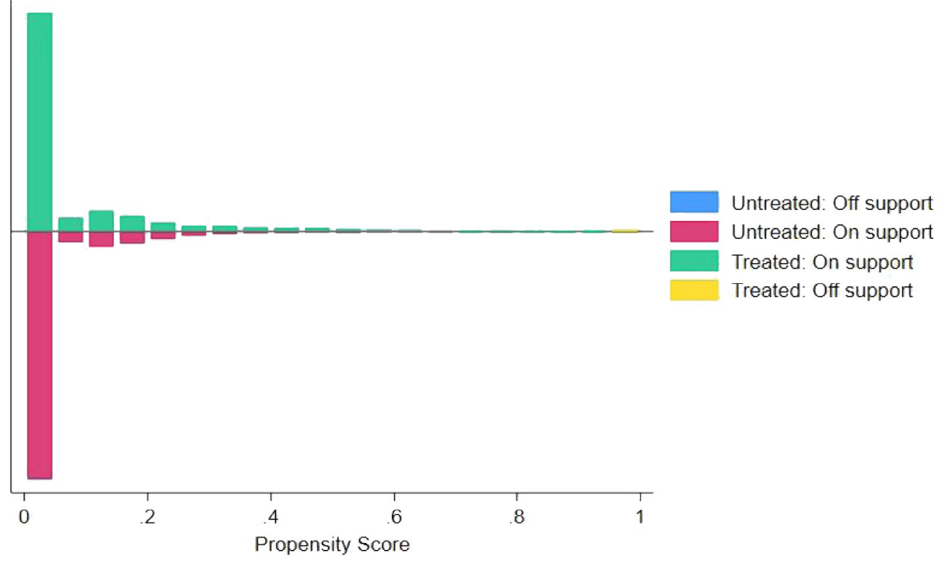
**Figure A1 | Common support of propensity score**
***Notes:*** This figure presents the common support of the propensity score for the groups with and without FH. The 1:4 nearest-neighbor matching within the caliper (0.05) is performed.

References

F. J. Rios, A. C. Montezano, L. L. Camargo, R. M. Touyz. Impact of environmental factors on hypertension and associated cardiovascular disease. Canadian Journal of Cardiology. Vol. 39, pg. 1229-1243, (2023). [↩]
Deepshikha, P. Mathur, Monika, V. Jhawat, S. Shekhar, R. Dutt, R. P. Singh. An overview of hypertension: pathophysiology, risk factors, and modern management. Current Hypertension Reviews. Vol. 21, pg. 64-81, (2025). [↩]
L. Yang, Z. Zhang, C. Du, L. Tang, X. Liu. Risk factor control and adherence to recommended Lifestyle among US hypertension patients. BMC Public Health. Vol. 24, pg. 2853, (2024). [↩]
K. Kario, A. Okura, S. Hoshide, M. Mogi. The WHO Global report 2023 on hypertension warning the emerging hypertension burden in globe and its treatment strategy. Hypertension Research. Vol. 47, pg. 1099-1102, (2024). [↩]
B. Zhou, R. M. Carrillo-Larco, G. Danaei, L. M. Riley, C. J. Paciorek, G. A. Stevens, J. Breckenkamp. Worldwide trends in hypertension prevalence and progress in treatment and control from 1990 to 2019: a pooled analysis of 1201 population-representative studies with 104 million participants. The Lancet. Vol. 398, pg. 957-980, (2021). [↩]
Y. Kokubo, S. Padmanabhan, Y. Iwashima, K. Yamagishi, A. Goto. Gene and environmental interactions according to the components of lifestyle modifications in hypertension guidelines. Environmental Health and Preventive Medicine. Vol. 24, pg. 19, (2019). [↩]
F. H. Messerli, B. Williams, E. Ritz. Essential hypertension. The Lancet. Vol. 370, pg. 591-603, (2007). [↩]
M. Slama, D. Susic, E. D. Frohlich. Prevention of hypertension. Current Opinion in Cardiology. Vol. 17, pg. 531-536, (2002). [↩]
O. M. Akpa, F. Made, A. Ojo, B. Ovbiagele, D. Adu, A. A. Motala, members of the CVD Working Group of the H3Africa Consortium. Regional patterns and association between obesity and hypertension in Africa: evidence from the H3Africa CHAIR study. Hypertension. Vol. 75, pg. 1167-1178, (2020). [↩]
G. O. Boateng, I. N. Luginaah, M. M. Taabazuing. Examining the risk factors associated with hypertension among the elderly in Ghana. Journal of Aging and Health. Vol. 27, pg. 1147-1169, (2015). [↩]
C. E. Margerison, J. Catov, C. Holzman. Pregnancy as a window to racial disparities in hypertension. Journal of Women’s Health. Vol. 28, pg. 152-161, (2019). [↩]
P. R. Rosenbaum, D. B. Rubin. The central role of the propensity score in observational studies for causal effects. Biometrika. Vol. 70, pg. 41-55, (1983). [↩]
C. J. Dzau, C. P. Hodgkinson. Precision hypertension. Hypertension. Vol. 81, pg. 702-708, (2024). [↩]
M. J. Samakosky, S. A. Norris. Alleviating the public health burden of hypertension: Debating precision prevention as a possible solution. Global Health Action. Vol. 17, pg. 2422169, (2024). [↩]
S. Goorani, S. Zangene, J. D. Imig. Hypertension: a continuing public healthcare issue. International Journal of Molecular Sciences. Vol. 26, pg. 123, (2024). [↩]
M. Takase, T. Hirata, N. Nakaya, M. Kogure, R. Hatanaka, K. Nakaya, ToMMo investigators. Associations of family history of hypertension, genetic, and lifestyle risks with incident hypertension. Hypertension Research. Vol. 48, pg. 2606-2617, (2025). [↩]
M. Ding, S. Ahmad, L. Qi, Y. Hu, S. N. Bhupathiraju, M. Guasch-Ferré, P. Kraft. Additive and multiplicative interactions between genetic risk score and family history and lifestyle in relation to risk of type 2 diabetes. American Journal of Epidemiology. Vol. 189, pg. 445-460, (2020). [↩]
B. Hezekiah, R. Pazoki. Physical Activity and favorable adiposity genetic liability reduce the risk of hypertension among high body mass individuals. Journal of the American Heart Association. Vol. 14, pg. e040701, (2025). [↩]
M. Niu, L. Zhang, Y. Wang, R. Tu, X. Liu, C. Wang, R. Bie. Lifestyle score and genetic factors with hypertension and blood pressure among adults in rural China. Frontiers in Public Health. Vol. 9, pg. 687174, (2021). [↩]
A. Abadie, G. W. Imbens. Large sample properties of matching estimators for average treatment effects. Econometrica. Vol. 74, pg. 235-267, (2006). [↩]
M. Mirzaei, M. Mirzaei, B. Bagheri, A. Dehghani. Awareness, treatment, and control of hypertension and related factors in adult Iranian population. BMC Public Health. Vol. 20, pg. 667, (2020). [↩]
Y. Chen, P. Hu, Y. He, H. Qin, L. Hu, R. Yang. Association of TyG index and central obesity with hypertension in middle-aged and elderly Chinese adults: a prospective cohort study. Scientific Reports. Vol. 14, pg. 2235, (2024). [↩]
J. A. Rassen, A. A. Shelat, J. Myers, R. J. Glynn, K. J. Rothman, S. Schneeweiss. One‐to‐many propensity score matching in cohort studies. Pharmacoepidemiology and Drug Safety. Vol. 21, pg. 69-80, (2012). [↩]
A. Abadie, D. Drukker, J. L. Herr, G. W. Imbens. Implementing matching estimators for average treatment effects in Stata. The Stata Journal. Vol. 4, pg. 290-311, (2004). [↩]
J. A. Smith, P. E. Todd. Reconciling conflicting evidence on the performance of propensity-score matching methods. American Economic Review. Vol. 91, pg. 112-118, (2001). [↩]
J. M. Wooldridge. Econometric Analysis of Cross Section and Panel Data. MIT Press, Cambridge, MA, (2002). [↩] [↩]
M. Frölich. Finite-sample properties of propensity-score matching and weighting estimators. Review of Economics and Statistics. Vol. 86, pg. 77-90, (2004). [↩]
R. H. Dehejia, S. Wahba. Causal effects in nonexperimental studies: Reevaluating the evaluation of training programs. Journal of the American Statistical Association. Vol. 94, pg. 1053-1062, 1999. [↩]
J. J. Heckman, H. Ichimura, P. E. Todd. Matching as an econometric evaluation estimator: Evidence from evaluating a job training programme. The Review of Economic Studies. Vol. 64, pg. 605-654, 1997. [↩]
E. C. Norton, H. Wang, C. Ai. Computing interaction effects and standard errors in Logistic regression and probit models. The Stata Journal. Vol. 4, pg. 154-167, 2004. [↩]
D. McFadden. Conditional [SH1] Logistic regression analysis of qualitative choice behavior. In Frontiers of Econometrics, P. Zarembka (Ed.), Academic Press, New York, 1974. [SH1] [↩]

Family history, lifestyle, and the prevalence of hypertension

Abstract

Introduction

Methods