Evaluating PPI as a Leading Indicator of U.S. CPI Inflation: Evidence from Lagged Regression Models, 1947-2025

Abstract

This study investigates whether the Producer Price Index (PPI) provides useful predictive information for Consumer Price Index (CPI) beyond the information contained in past CPI. Using the U.S. PPI and CPI data between 1947 and 2025, I constructed lagged regression models of year-over-year (YoY) inflation in Python and evaluated them on a chronologically held-out 2010 – 2025 test period. The combined model, which uses lagged PPI together with lagged CPI, predicts CPI YoY inflation accurately out-of-sample (R² ≈ 0.97; RMSE ≈ 0.32 pp). However, a baseline comparison shows that most of this accuracy comes from the persistence of inflation itself. Adding lagged PPI to a CPI only autoregressive baseline reduces out-of-sample RMSE by about 2%, but a Diebold-Mariano test cannot distinguish this improvement from zero under either squared-error (p = 0.53) or absolute-error loss (p = 0.86), and the same result holds under expanding window validation. While lagged PPI terms are statistically significant in-sample, the gain in out-of-sample forecast accuracy from adding PPI to what past CPI already reveals is not statistically distinguishable from zero. This pattern holds across lag lengths of 1-12 months. Forecast accuracy is also not uniform over time with RMSE rising by roughly 26% during the COVID-19 disruption of 2020-2021 relative to the pre-COVID test years. The hypothesis that PPI leads CPI at a measurable lag is therefore supported only in a limited sense in that lagged PPI contains statistically detectable in-sample information about CPI inflation, but this does not translate into a statistically detectable improvement in out-of-sample forecasting.

Keywords: CPI, PPI, inflation, regression, modeling, lagged.

Introduction

Inflation is an increase in the price of goods and services over time and is an important measure of economic stability. Federal Reserve policymakers study changes in inflation by monitoring several key price indexes^1,2. The Bureau of Labor Statistics (BLS) measures labor market activity, working conditions, price changes, and productivity in the U.S. economy to support public and private decision making. Inflation affects the purchasing power of money, the value of investments, and the cost of goods and services for consumers and businesses. Economists track inflation through several indices, the most notable being the Producer Price Index (PPI) and the Consumer Price Index (CPI).

The first is the Producer Price Index (PPI). PPI measures the average change over time in the selling prices received by domestic producers for their output. PPI tracks prices at the wholesale/production level (before goods reach consumers). BLS publishes PPI monthly.

The second is the Consumer Price Index (CPI), which measures the average change over time in the prices paid by consumers for goods and services. CPI can be used to index the real value of wages, salaries, and pensions, to regulate prices, and to deflate monetary magnitudes to show changes in real values. In most countries, CPI is one of the most important national economic statistics and macroeconomic variables.

Firms normally pass on their production costs to consumers, so changes in producer level prices will typically be seen before changes in consumer level prices. In other words, increasing production costs for a company should cause an increase in consumer prices. Research has been conducted to support this premise and indicates that the PPI represents a leading indicator for the CPI with a delay of a few months. Depending upon the economic environment, the strength and consistency of this lead lag relationship may vary across geographies, industries, and time periods.

Since it is assumed that the change in costs associated with the producer will be transferred to the consumer, it follows that the PPI would predict the CPI. Therefore, when costs for producers rise, the price to consumers should also eventually rise. Many studies have examined this relationship indicating that producer prices lead to consumer prices by several months.

This paper adds on to this pool of research by testing whether PPI serves as a reliable predictor of CPI using historical U.S. inflation data between 1947 and 2025. By using a lagged time index of PPI and regression modeling, this study evaluates the strength of this predictive relationship.

Therefore, this paper seeks to evaluate the following hypothesis – PPI is a leading predictor of CPI accounting for a measurable time lag.

Related Work and Literature Review

Various researchers have studied the relationship between CPI and PPI.³ found that there is a long-term stable relationship between the CPI and the PPI. They also found that CPI is influenced by its own past values, with both short-term fluctuations and long-term effects contributing to its movement.⁴ analyzed the relationship between CPI and PPI for Mexico from 1981 to 2009 and found a bi-directional relationship between CPI and PPI where CPI is leading PPI in short periods (1 to 7 months), while for longer periods (8 to 32 months), PPI was found as the leading variable.⁵ studied the relationship between PPI, enterprise commodity price index, M2, and CPI through the Granger causality test and cointegration theory and indirectly confirmed that PPI is one-way causality of CPI.⁶ used China’s CPI and PPI data from January 2001 to August 2008 to conduct empirical research. The Granger causality test showed that there was one-way transmission from CPI to PPI and CPI Granger causes the change in PPI with the latter reacting to the former with a time lag of 1-3 months.⁷ used the same data as⁶ to find the Granger reason for each other in the short and long term. They concluded that CPI and PPI are complex nonlinear causality.

The international evidence on the PPI-CPI lead lag relationship is decidedly mixed.⁸ found a robust long-run relationship between producer and consumer prices in Pakistan using the auto-regressive distributive model (ARDL) and found that the feedback influence from PPI to CPI is stronger or dominating as compared to feedback from CPI to PPI. In contrast with earlier international evidence,⁹ found that PPI has a significant predictive content for the subsequent development of CPI inflation forecasts in Mexico.¹⁰ found bi-directional causality between producer and consumer prices in both Turkey and the United Kingdom. Working in the frequency domain,¹¹ found that in Australia producer prices do not Granger-cause consumer prices at any frequency and consumer prices instead lead producer prices.

In China,¹² applied a rolling-window bootstrap causality test and found that the direction of causality between PPI and CPI shifts over time rather than remaining fixed. At the sectoral level,¹³ found no causal link from producer prices to consumer prices for South African beef, with causality for other meats running from consumer to producer prices.

Taken together, these studies show that the direction, strength, and timing of price transmission vary substantially across countries, sectors, periods, and methods thereby motivating a careful, baseline-controlled test of PPI’s predictive content for the United States.

One of the first studies that analyzed the relationship between producer and consumer prices was “Do Producer Prices Lead Consumer Prices?”¹⁴, published in the Economic Review of the Federal Reserve Bank of Kansas City in 1995. Clark studied whether increases in PPI cause correlating increases in future CPI. Clark used forecasting models such as vector autoregressions (VAR’s) and focused on the data between 1958 and early 1995 and found that empirical evidence shows that the production chain only weakly links consumer prices to producer prices. In addition, he found that PPI changes sometimes help predict CPI changes but fail to do so systematically.  Clark’s conclusion has since been corroborated in the peer-reviewed literature.¹⁵ find unidirectional causality from producer to consumer prices across the G7,¹⁶ report the same direction for Malaysia, and¹⁷ finds it in Finland and France but bidirectional causality in Germany and none in the Netherlands or Sweden thereby reinforcing Clark’s central point that any lead is real but neither uniform nor systematic.

Another study that explores inflation prediction using economic indicators is “Using economic indicators to create an empirical model of inflation” by¹⁸. This research study also looks to forecast inflation (using CPI), through historical economic data. They analyzed correlations between CPI and 50 economic indicators and found that variables such as average gasoline prices, the U.S. import price index, and five-year market expected inflation displayed the strongest relationships with CPI. They found that a linear regression consisting of the average gasoline price, average import price, and 5-year treasury inflation protected securities (TIPS) could predict CPI one month ahead within 0.107 units of the expected CPI. Kasera also found one limitation of the model is its inaccuracy in predicting inflation during highly chaotic economic times such as the 2008 financial crisis and COVID. The broader peer-reviewed literature on indicator-based inflation forecasting reaches a similar conclusion –¹⁹ show that although individual activity indicators can forecast US inflation, their advantage over simple univariate benchmarks is unstable across periods, which anticipates the pattern found here.

A related literature applies machine learning to inflation forecasting.²⁰ showed that machine learning methods with large sets of predictors such as random forests can improve U.S. inflation forecasts by as much as 30% in squared-error terms relative to the standard benchmarks.²¹ compared regression-based and machine learning approaches for predicting the U.S. CPI from macro financial inputs, and²² found that long short-term memory (LSTM) recurrent neural networks outperform linear autoregressive and random-walk benchmarks for monthly U.S. inflation, while cautioning that such models are prone to overfitting on short, persistent macroeconomic series. These methods improve accuracy at a cost in transparency, which motivates the simple, interpretable regression design used here.

This paper contributes to the US PPI-CPI relationship in four specific ways. First, rather than testing in-sample Granger causality, which is the dominant approach in the country studied above, this research paper evaluates PPI’s predictive content out-of-sample, on a strictly chronological 2010-2025 hold-out period, using one of the longest samples in this literature with U.S. data spanning 1947-2025. Second, it measures PPI’s incremental value against an autoregressive CPI baseline, so that the persistence of inflation itself is not mistakenly credited to PPI, a comparison many prior studies omit. Third, it does so with a transparent, fully specified linear model whose lag structure is selected by information criteria computed on the training data alone, and whose forecasts are evaluated both at a fixed 2010 origin and by expanding-window validation in which the model is refit every month. Time-aware cross-validation is used only to choose the ridge penalty within the training window and not to evaluate the forecasts themselves. Together these provide an interpretable complement to the black-box machine learning approaches surveyed above. Fourth, the incremental contribution of PPI is assessed with a formal test of equal predictive accuracy rather than by comparing error metrics informally.

Methodology and Data Analysis

To evaluate whether lagged changes in the Producer Price Index (PPI) predict changes in the Consumer Price Index (CPI), I utilized PPI and CPI data from FRED^1,2 between 1947 and 2025.

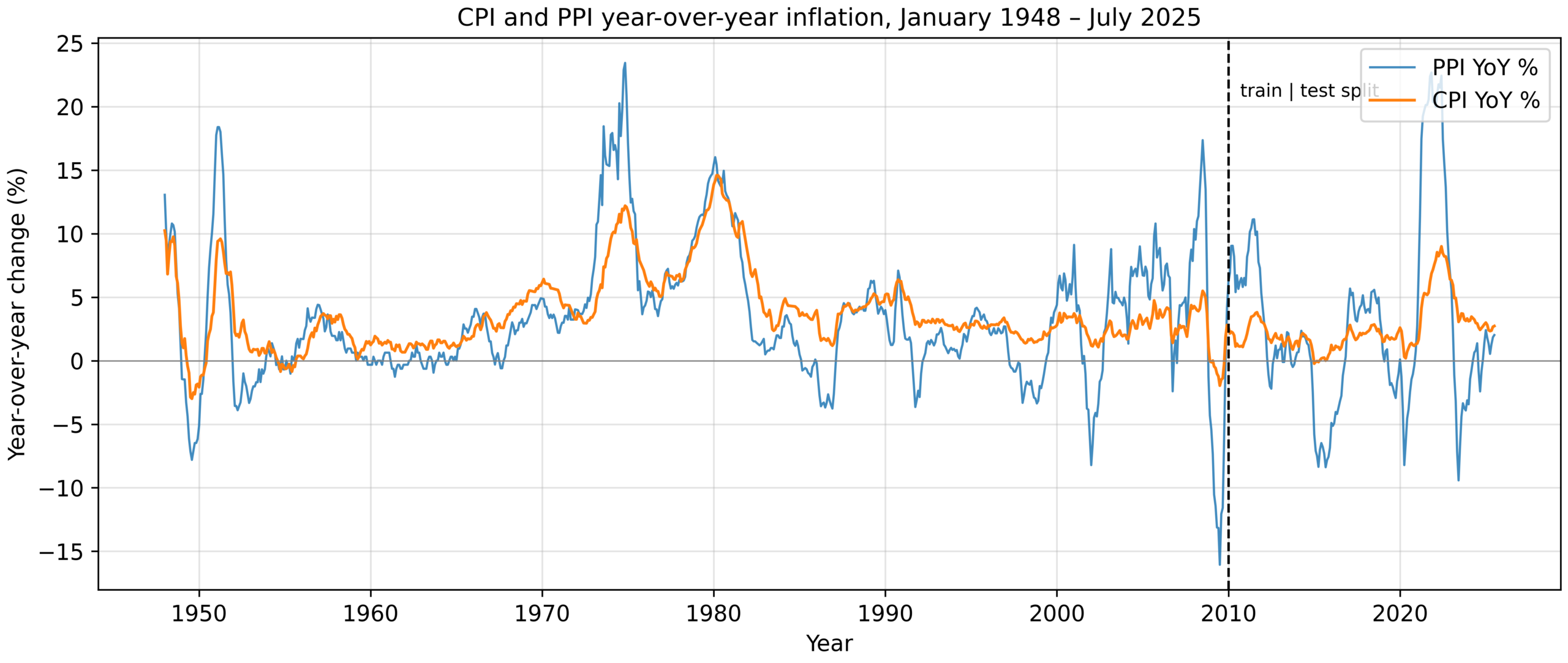
The underlying CPI and PPI index data run from January 1947 to July 2025. Because the analysis uses year-over-year changes, each observation is a comparison with the same month one year earlier, so the first year of index data is consumed in constructing the first inflation observation and the year-over-year series therefore begins in January 1948. Figure 1 plots the two series in year-over-year terms over the full sample, together with the point at which the data are split into training and test periods. After the additional lagged predictors are constructed, the estimation sample begins in December 1948.

First, I used pandas for data analysis and manipulation. Monthly CPI and PPI data were imported from the CSV files and placed in one data set using a time index (observation_date). Pandas were also used to sort observations chronologically, compute year-over-year (YoY) percentage changes for CPI and PPI, construct lagged variables for PPI (1–12 months) and CPI (1–2 months), and remove missing values generated by differencing and lagging.

# Load monthly CPI and PPI series and align them on date
cpi_df = pd.read_csv('data/cpi.csv')
ppi_df = pd.read_csv('data/ppi.csv')
joined_df = pd.merge(cpi_df, ppi_df, on='observation_date', how='inner')
joined_df = joined_df.rename(columns={'CPIAUCSL': 'cpi', 'PPIACO': 'ppi'})
joined_df['observation_date'] = pd.to_datetime(joined_df['observation_date'])
joined_df = joined_df.sort_values('observation_date')
 
# Convert both indices to year-over-year (YoY) percentage changes
joined_df['cpi_pct'] = joined_df['cpi'].pct_change(12) * 100
joined_df['ppi_pct'] = joined_df['ppi'].pct_change(12) * 100
 
# Build lagged PPI features (1-11 months) and lagged CPI terms (1-2 months)
for lag in range(1, 12):
    joined_df[f'ppi_pct_lag{lag}'] = joined_df['ppi_pct'].shift(lag)
joined_df['cpi_lag1'] = joined_df['cpi_pct'].shift(1)
joined_df['cpi_lag2'] = joined_df['cpi_pct'].shift(2)
joined_df = joined_df.dropna()

Next, I used scikit-learn for regression modeling. RidgeCV (Ridge Regression with built-in Cross Validation) was used to estimate the relationship between CPI and lagged inflation variables. Ridge regression is a statistical regularization technique. It corrects for overfitting on training data in machine learning models. Because the data form a time series, the cross-validation used to select the regularization strength was performed with scikit-learn’s TimeSeriesSplit (five-folds), which always validates on periods that come after the periods used for fitting, so no future information leaks into model selection. I used ridge regression over ordinary least squares (OLS) to address multicollinearity (the concept that when two or more independent variables are highly correlated, it is hard to tell each variable’s individual effect on the outcome) among lagged inflation indicators.

I split the data chronologically in January 2010, with no shuffling. Observations through December 2009 formed the training set with 733 monthly observations, where the year-over-year transformation and lag construction consume the first months of data, so training effectively begins in December 1948. Observations from January 2010 through July 2025 formed the test set with 187 monthly observations.

# Chronological split at January 2010 - no shuffling, so no future
# observation can ever appear in the training set
SPLIT_DATE = "2010-01-01"
train_mask = joined_df['observation_date'] < SPLIT_DATE
test_mask = ~train_mask
 
X = joined_df[['ppi_pct_lag1', 'ppi_pct_lag2', 'cpi_lag1', 'cpi_lag2']]
y = joined_df['cpi_pct']
X_train, X_test = X[train_mask], X[test_mask]
y_train, y_test = y[train_mask], y[test_mask]
 
# Time-aware cross-validation: each validation fold comes strictly
# after the data used to fit it
tscv = TimeSeriesSplit(n_splits=5)
alphas = [0.01, 0.1, 1.0, 10.0, 100.0]
model = RidgeCV(alphas=alphas, cv=tscv)
model.fit(X_train, y_train)

A chronological split is essential for evaluating a time-series forecast. A random train/test split would place future observations in the training data, allowing the model to “see the future” and overstating its true out-of-sample accuracy.

A single chronological split still estimates the coefficients once, in January 2010, and then holds them fixed for the following 15.5 years, which is not how a forecast would be produced in practice. I also evaluated the models by expanding-window (rolling-origin) validation so that for every month in the test period the model is refit on all data available up to that month and then used to predict the next observation. This produces 187 genuinely recursive one-month-ahead forecasts and is reported alongside the fixed-origin results.

To isolate the incremental predictive value of PPI, I estimated three separate models on the same training and test sets:

• an autoregressive baseline using only the first two lags of CPI inflation,
• a model using only the first two lags of PPI inflation, and
• a combined model containing both sets of predictors.

Because YoY CPI inflation is highly persistent, a high R² for a model that includes lagged CPI terms does not, by itself, demonstrate that PPI adds predictive value. Comparing the out-of-sample errors of the combined model against the CPI-only baseline measures how much forecasting accuracy PPI adds beyond the information already contained in past CPI values.

RidgeCV searched for a candidate grid of regularization strengths α ∈ {0.01, 0.1, 1, 10, 100} and selected α = 0.01 for the main model. Predictors were not standardized prior to fitting, and every predictor is a year-over-year inflation rate measured in the same units (percentage points) and on a comparable scale. So, the ridge penalty already treats the coefficients symmetrically. Standardization matters most when predictors are measured on very different scales, which is not the case here. The number of PPI lags in the main specification was itself chosen by the lag-length comparison reported in Table 1. On the training set, the Bayesian Information Criterion (BIC) is minimized at two lags, and two lags also give the lowest out-of-sample RMSE and MAE. The main model therefore uses PPI lags of one and two months together with CPI lags of one and two months. The estimated regression model can be written as:

CPIt = β0 + β1PPIt−1 + β2PPIt−2 + β3CPIt−1 + β4CPIt−2 + εt

Where CPI_t and PPI_t denote YoY % changes in month t and ε_t is the error term.

The ridge coefficients fitted on the training data are β0 = 0.072, β1 = 0.090, β2 = −0.076, β3 = 1.240, and β4 = −0.272.

These are the penalized (ridge) estimates and the unpenalized OLS estimates used for the inference in Table 3 are reported separately there and are almost identical, because the selected penalty (α = 0.01) is very small.

I also used scikit-learn to calculate the Coefficient of Determination or R², which is a statistical measure that represents how much of the variation of the dependent variable is explained by an independent variable in a regression model as shown below:

• SS_residuals – The sum of squares of the residuals (the unexplained error of the model)
• SS_total – The total sum of squares

R² ranges from 0 to 1, where 1 indicates a perfect fit of the model to the data.

In addition to R², I evaluated forecasting accuracy on the held-out test set using three standard error metrics – root mean squared error (RMSE), mean absolute error (MAE), and mean absolute percentage error (MAPE). RMSE and MAE are expressed in percentage points of year-over-year CPI inflation. RMSE penalizes large errors more heavily, while MAE reflects the typical size of a prediction error. MAPE expresses the average error as a percentage of the actual value.

A lower RMSE does not by itself establish that one model forecasts better than another, because the difference may be within sampling noise. To test this formally, I used the Diebold–Mariano test²³, which evaluates the null hypothesis that two sets of forecasts have equal expected loss. The test is applied to the baseline and combined models under both squared-error and absolute-error loss and is reported with the Harvey–Leybourne–Newbold small-sample correction²⁴.

# Forecast accuracy on the held-out test set
y_pred = model.predict(X_test)
 
r2   = r2_score(y_test, y_pred)
rmse = np.sqrt(mean_squared_error(y_test, y_pred))
mae  = mean_absolute_error(y_test, y_pred)
mape = np.mean(np.abs((y_test - y_pred) / y_test)) * 100
 
print(f"R2:   {r2:.4f}")
print(f"RMSE: {rmse:.4f} pp")
print(f"MAE:  {mae:.4f} pp")
print(f"MAPE: {mape:.2f}%")

Next, I used matplotlib to visualize relationships between variables and to assess model performance. There were two primary plots generated. The first was the Actual vs. Predicted CPI scatterplot, which compares predicted CPI YoY inflation against actual values in the test sample.

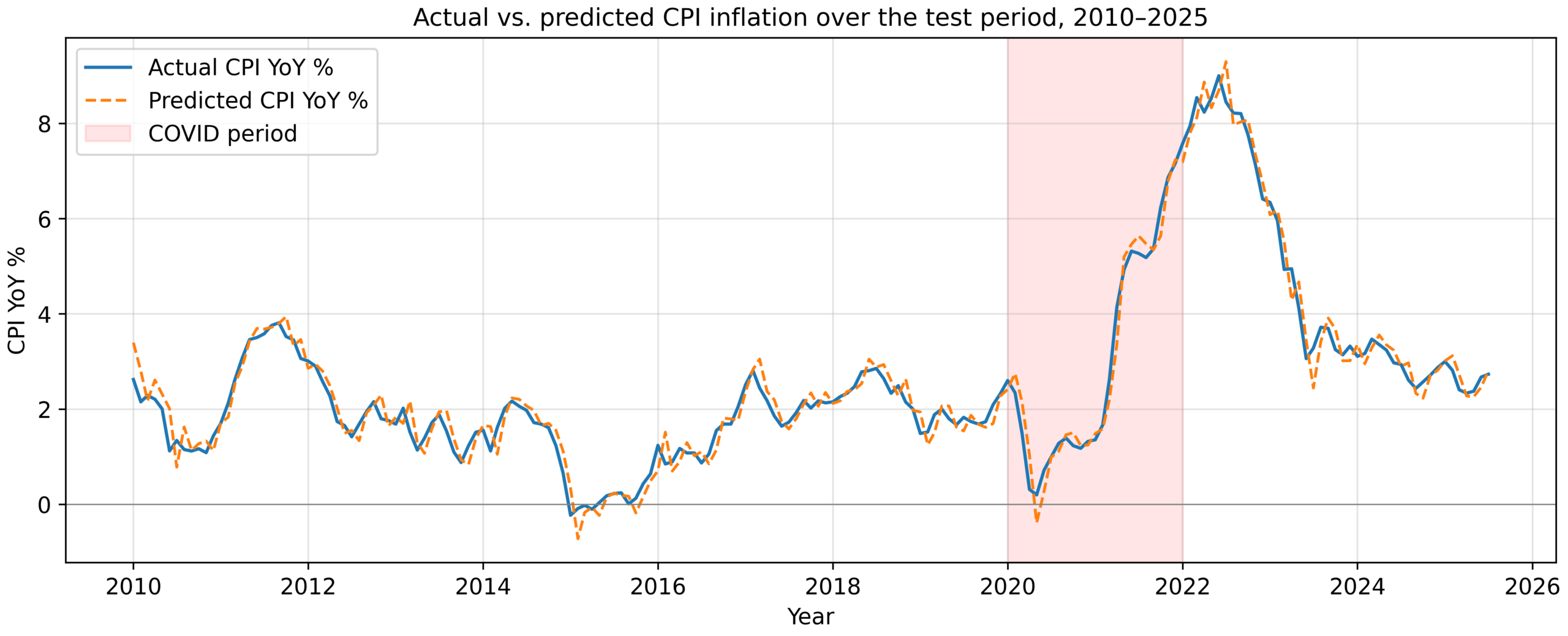
A 45-degree line was added for reference to visually assess accuracy and correlation strength. Clusters of data around this line indicate a strong fit. The second was the Time-Series Comparison plot, which visualizes actual and predicted CPI YoY inflation over time for the duration of the test period. This allows me to inspect model performance across different economic conditions, including periods that had rapid rates of inflation/disinflation.

# Actual vs. predicted scatter for the test period
fig, ax = plt.subplots(figsize=(7, 5.5))
ax.scatter(y_test, y_pred, alpha=0.7)
ax.plot([y_test.min(), y_test.max()],
        [y_test.min(), y_test.max()], 'r--', lw=2)
ax.set_xlabel('Actual CPI YoY %')
ax.set_ylabel('Predicted CPI YoY %')
ax.grid(True)
 
# Actual vs. predicted over time, with the COVID window shaded
fig5, ax5 = plt.subplots(figsize=(11, 4.6))
td = joined_df.loc[test_mask, 'observation_date']
ax5.plot(td, y_test, label='Actual CPI YoY %')
ax5.plot(td, y_pred, label='Predicted CPI YoY %', ls='--')
ax5.axvspan(pd.Timestamp('2020-01-01'), pd.Timestamp('2022-01-01'),
            color='red', alpha=0.10, label='COVID period')
ax5.legend(); ax5.grid(True, alpha=0.35)

Results

Model performance for every PPI lag length from 1 to 12 months is summarized in Table 1 below, so that the full set of specifications tested is visible rather than a selected subset. Figures 2 through 4 illustrate the fit of the main model and Figures 5 and 6 present the lag-length analysis. The analysis illustrates that the combined model explains roughly 97% of the variation in CPI YoY changes using lagged PPI together with lagged CPI features. As the baseline comparison below shows, most of this explanatory power comes from the persistence of inflation itself rather than from PPI alone.

PPI lags (k)	R2	RMSE (pp)	MAE (pp)	AIC	BIC
1	0.9711	0.3265	0.2536	648.2	666.5
2	0.9725	0.3186	0.2503	628.9	651.8
3	0.9717	0.3232	0.2540	628.4	655.9
4	0.9710	0.3268	0.2553	629.6	661.7
5	0.9711	0.3267	0.2552	631.6	668.3
6	0.9710	0.3268	0.2546	632.8	674.0
7	0.9707	0.3286	0.2556	633.4	679.2
8	0.9710	0.3272	0.2526	630.0	680.4
9	0.9706	0.3292	0.2539	631.5	686.5
10	0.9704	0.3303	0.2548	632.9	692.4
11	0.9704	0.3302	0.2550	634.9	699.0
12	0.9706	0.3292	0.2549	636.7	705.4

The forecast errors on the 2010-2025 test set are small in absolute terms. For the main two-lag specification, the RMSE is 0.32 percentage points, and the MAE is 0.25 percentage points, implying that the model’s predictions are typically within about a quarter of a percentage point of actual year-over-year inflation. The MAPE is high (around 39%) because year-over-year inflation was close to zero during parts of the test period (for example, much of 2015), which inflates percentage-based error measures. RMSE and MAE are therefore the more informative measures of accuracy here.

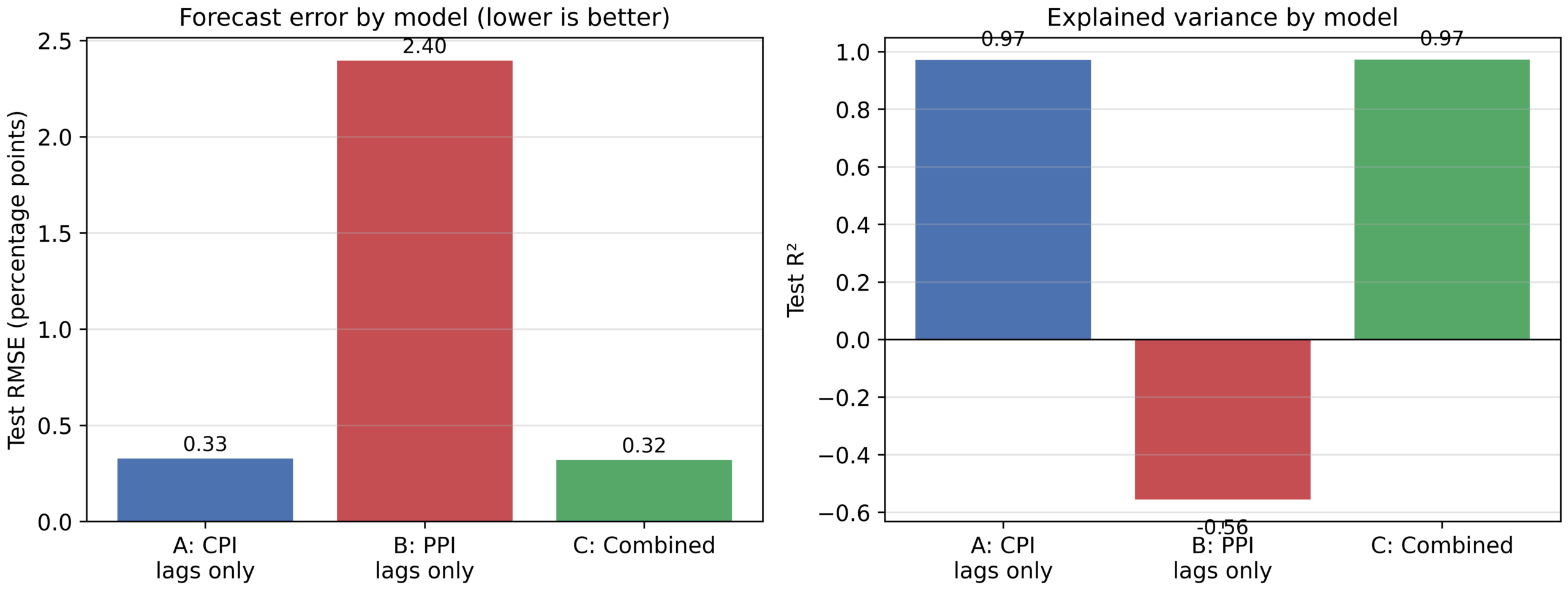
To separate the contribution of PPI from the persistence of CPI itself, Table 2 compares the three models on the same 2010–2025 test set. The CPI-only autoregressive baseline Model A already achieves an R² of 0.9711, with an RMSE of 0.3266 percentage points and an MAE of 0.2528 percentage points. The PPI-only model Model B performs poorly out-of-sample: its negative R² means it predicts worse than simply using the test-period mean. Adding the lagged PPI features to the baseline Model C improves both error measures, reducing RMSE by 2.18% in relative terms (from 0.3266 to 0.3195 percentage points) and MAE by 0.55% (from 0.2528 to 0.2514 percentage points). The direction of the improvement is therefore consistent across both loss functions, but its size is small.

Model	R2	RMSE (pp)	MAE (pp)
A: CPI lags only (baseline)	0.9711	0.3266	0.2528
B: PPI lags only	−0.5558	2.3953	1.8866
C: Combined (PPI + CPI lags)	0.9723	0.3195	0.2514

# Three models fitted on identical training and test sets
cpi_lag_cols = ['cpi_lag1', 'cpi_lag2']
ppi_lag_cols = ['ppi_pct_lag1', 'ppi_pct_lag2']
 
def fit_and_score(cols, label):
    m = RidgeCV(alphas=alphas, cv=TimeSeriesSplit(n_splits=5))
    m.fit(X_train[cols], y_train)
    p = m.predict(X_test[cols])
    return {'label': label,
            'r2':   r2_score(y_test, p),
            'rmse': np.sqrt(mean_squared_error(y_test, p)),
            'mae':  mean_absolute_error(y_test, p)}
 
results = [
    fit_and_score(cpi_lag_cols, 'A: CPI lags only'),
    fit_and_score(ppi_lag_cols, 'B: PPI lags only'),
    fit_and_score(cpi_lag_cols + ppi_lag_cols, 'C: combined'),
]
 
# The evidence that PPI helps is the error reduction of C over A
rmse_a, rmse_c = results[0]['rmse'], results[2]['rmse']
print(f"RMSE reduction of combined over CPI-only baseline: "
      f"{(rmse_a - rmse_c) / rmse_a * 100:.2f}%")

A Diebold–Mariano test of equal predictive accuracy cannot reject the null that the two models forecast equally well, under either squared-error loss (p = 0.53) or absolute-error loss (p = 0.86). The improvement from adding PPI is not statistically distinguishable from zero. This comparison shows that essentially all of the model’s forecasting accuracy comes from the autocorrelation of inflation itself.

Figure 2 presents the same comparison visually: Models A and C are nearly indistinguishable, while Model B is far worse on both measures. The dominance of the autoregressive terms is consistent with the peer-reviewed evidence on US inflation persistence, which finds inflation strongly serially correlated even as the degree of persistence has shifted over time^25,26.

Because the fixed-origin split holds the coefficients constant from 2010 onward, I repeated the comparison using expanding-window validation, refitting both models every month on all data available up to that point. The conclusion is unchanged and the baseline achieves an RMSE of 0.3271 percentage points and the combined model 0.3193, and a Diebold–Mariano test again fails to reject equal predictive accuracy (p = 0.43 under squared-error loss, p = 0.74 under absolute-error loss). That the recursive and fixed-origin results agree so closely indicates that the finding is not an artefact of estimating the coefficients once in 2010.

Because ridge regression does not produce valid standard errors or p-values, statistical significance was assessed with a separate robustness check. The combined model was re-estimated by ordinary least squares with Newey–West (HAC) standard errors²⁷ (six lags), which remain valid under the autocorrelation (i.e. the errors are correlated over time) and heteroskedasticity (i.e. the variance of the errors is not constant) present in monthly inflation data. This regression is estimated on the training sample only, that is on the 733 monthly observations from December 1948 to December 2009, so its coefficients describe the in-sample relationship over that period rather than the full 1947-2025 span.

The full set of coefficients, HAC standard errors, z-statistics, p-values and 95% confidence intervals is reported in Table 3. Both PPI lags are individually significant in this specification (first lag 0.0898, p = 0.003; second lag −0.0759, p = 0.022), and the CPI autoregressive terms are highly significant (p < 0.001). Because a twelve-month overlapping year-over-year difference can leave autocorrelation out to roughly eleven lags, I checked that the conclusion does not depend on the HAC bandwidth and the first PPI lag remains significant at six, twelve and twenty-four lags (p = 0.003, 0.005 and 0.012 respectively). Note that the coefficients in Table 3 are unpenalized OLS estimates used for inference and are distinct from the ridge coefficients reported in the Methodology, although at α = 0.01 the two sets are almost identical. In-sample statistical significance, however, is not the same as out-of-sample forecasting value. As the baseline comparison in Table 2 shows, the accuracy gain from adding PPI is not statistically distinguishable from zero. Accordingly, this paper claims only that PPI carries a detectable in-sample lead and does not claim that PPI improves out-of-sample forecasts of CPI.

Term	Coefficient	Std. error	z	p-value	95% CI
Intercept	0.0723	0.028	2.57	0.010	[0.017, 0.127]
PPI t−1	0.0898	0.031	2.92	0.003	[0.030, 0.150]
PPI t−2	−0.0759	0.033	−2.29	0.022	[−0.141, −0.011]
CPI t−1	1.2405	0.052	23.98	<0.001	[1.139, 1.342]
CPI t−2	−0.2722	0.052	−5.28	<0.001	[−0.373, −0.171]

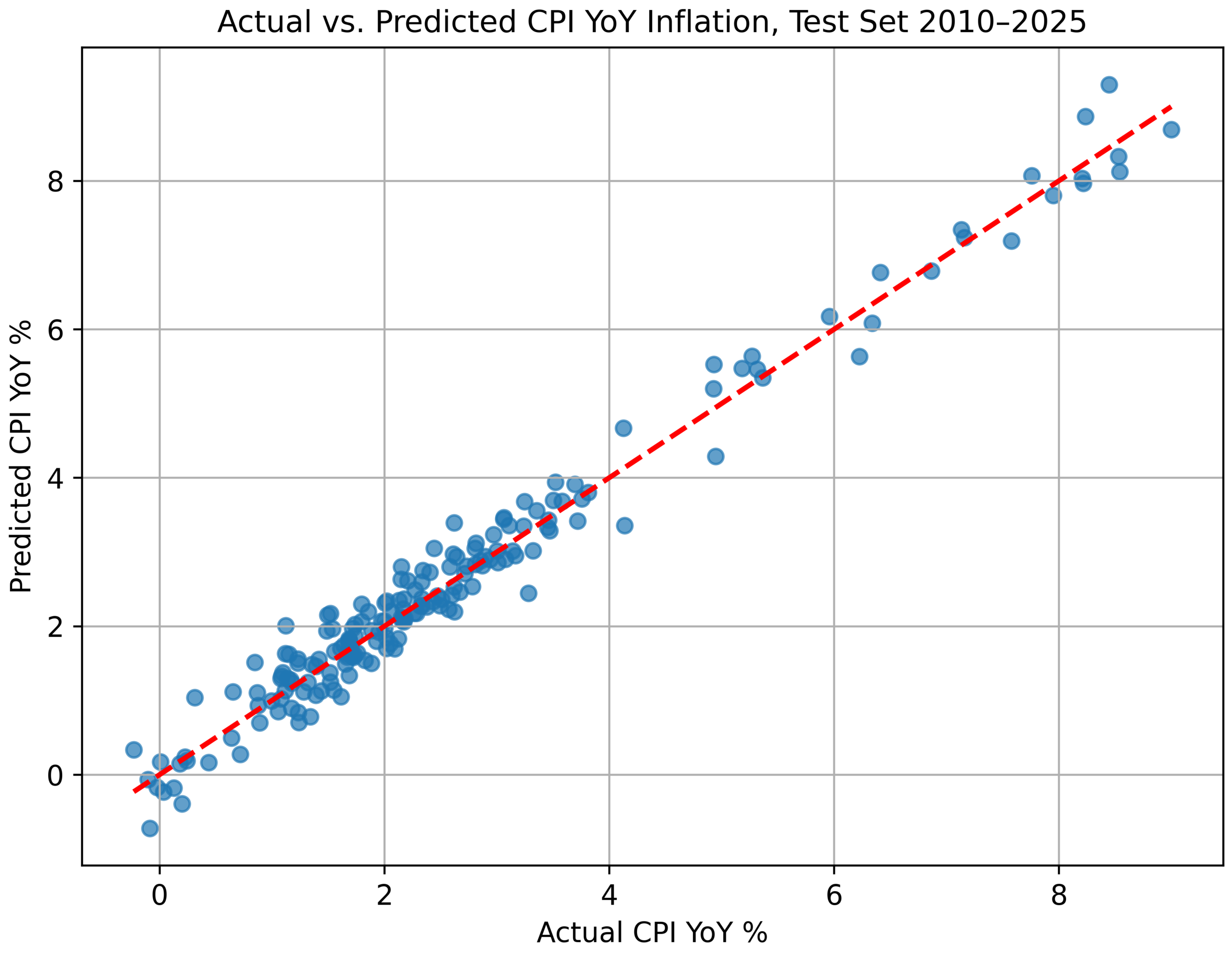
Looking at the Actual vs. Predicted CPI scatterplot (Figure 3), the points are all clustered closely around the 45-degree line, indicating accurate predictions across the different time periods. Figure 4 shows the same predictions plotted over time, which makes the model’s behavior during the 2021–2022 inflation surge easier to inspect.

Rather than selecting the lag length by visually inspecting where the correlation between PPI and CPI appears to peak, I compared models with PPI lag lengths of 1 through 12 months using out-of-sample error and information criteria computed on the training set (Figure 5).

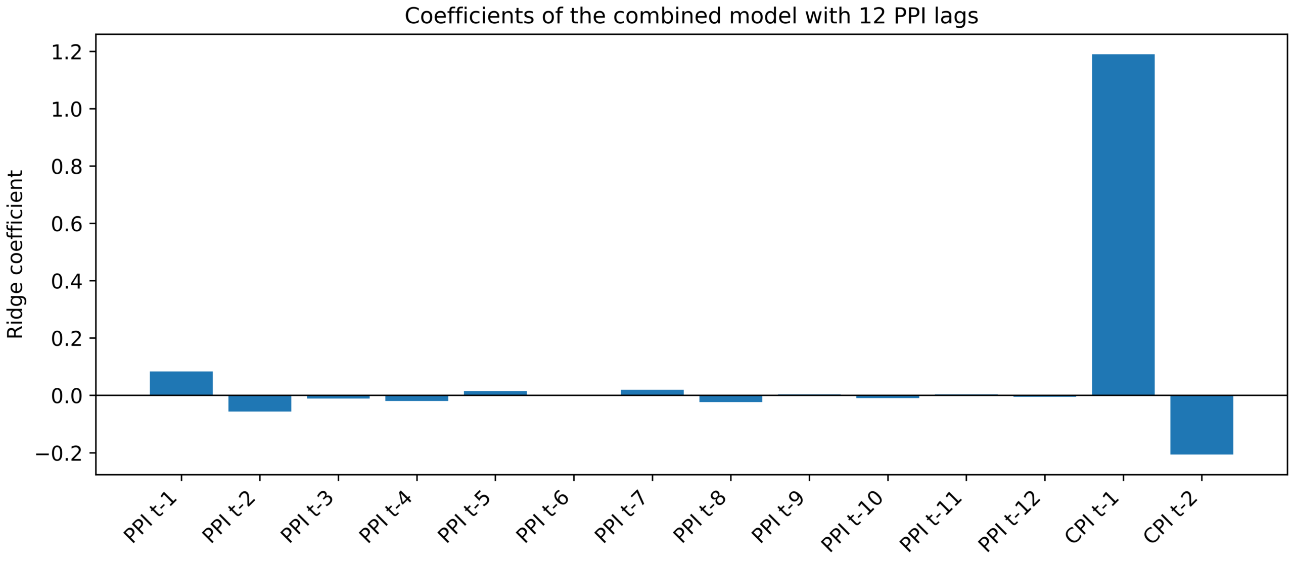
Out-of-sample RMSE is flat across all lag lengths, varying by less than 0.02 percentage points, and the 12-month specification performs no better than shorter ones (Table 1). The Bayesian Information Criterion (BIC), computed from an unpenalized OLS refit on the training data, is clearly minimized at two lags (651.8, against 655.9 at three lags). The Akaike Information Criterion is effectively uninformative here and it varies by less than two units across k = 2, 3 and 8 (628.9, 628.4 and 630.0), a range far too narrow to discriminate between specifications. Out-of-sample RMSE and MAE both also reach their minimum at two lags. Every criterion that discriminates therefore points to a short lag structure of two months, which is the specification used in the main model. Figure 6 shows the coefficients of a model containing all 12 PPI lags and the CPI autoregressive terms dominate, and every PPI coefficient is close to zero, consistent with the baseline comparison in Table 2.

# Compare PPI lag lengths 1-12 on a common sample, scoring each by
# out-of-sample error and by AIC/BIC computed on the training set
for k in range(1, MAX_LAG + 1):
    cols = [f'ppi_pct_lag{l}' for l in range(1, k + 1)] + cpi_lag_cols
    tr_k = df_sweep['observation_date'] < SPLIT_DATE
    Xk, yk = df_sweep[cols], df_sweep['cpi_pct']
 
    mk = RidgeCV(alphas=alphas, cv=TimeSeriesSplit(n_splits=5))
    mk.fit(Xk[tr_k], yk[tr_k])
    pk = mk.predict(Xk[~tr_k])
 
    ols = sm.OLS(yk[tr_k], sm.add_constant(Xk[tr_k])).fit()
    lag_results.append({'k': k,
                        'rmse': np.sqrt(mean_squared_error(yk[~tr_k], pk)),
                        'aic': ols.aic, 'bic': ols.bic})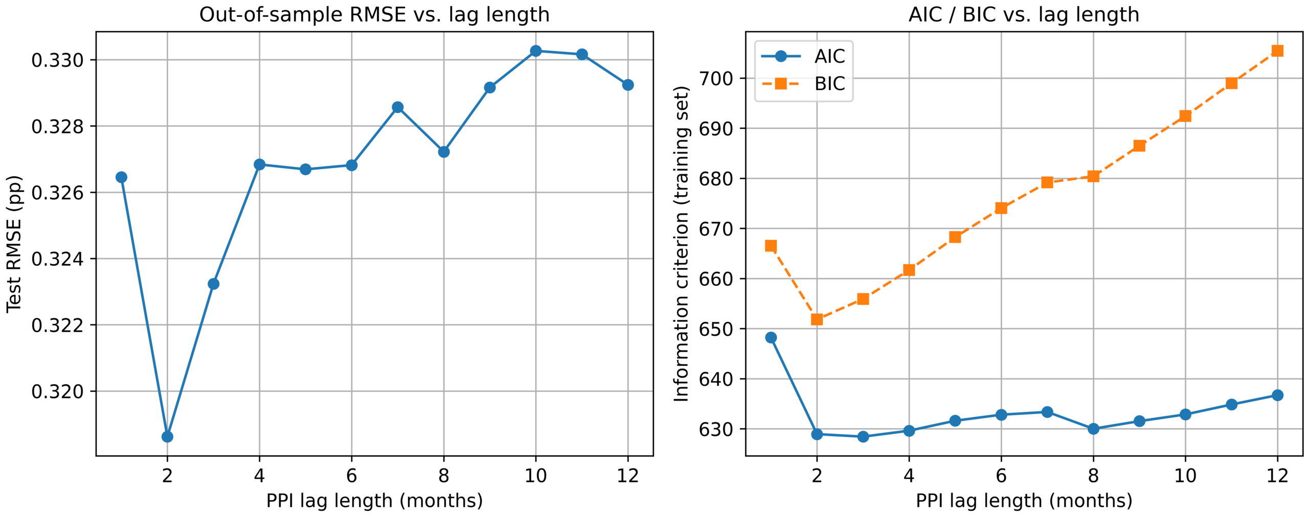

Finally, to examine how the model performed during the COVID-19 disruption, the test set was split into pre-COVID (2010–2019), COVID (2020–2021), and post-COVID (2022–2025) sub-periods, and the main model’s forecast errors were computed separately as illustrated in Table 4.

# Split the test set into COVID sub-periods and score each separately
subperiods = {
    'Pre-COVID (2010-2019)':  (test_dates_all < '2020-01-01'),
    'COVID (2020-2021)':      (test_dates_all >= '2020-01-01') &
                              (test_dates_all < '2022-01-01'),
    'Post-COVID (2022-2025)': (test_dates_all >= '2022-01-01'),
}
for name, m in subperiods.items():
    yt, yp = y_test_r[m], y_pred_s[m]
    print(f"{name:<24} n={m.sum():>4} "
          f"R2={r2_score(yt, yp):.4f} "
          f"RMSE={np.sqrt(mean_squared_error(yt, yp)):.4f}")

Period	n	R²	RMSE (pp)	MAE (pp)
Pre-COVID (2010–2019)	120	0.8798	0.2962	0.2312
COVID (2020–2021)	24	0.9712	0.3718	0.2884
Post-COVID (2022–2025)	43	0.9764	0.3490	0.2874

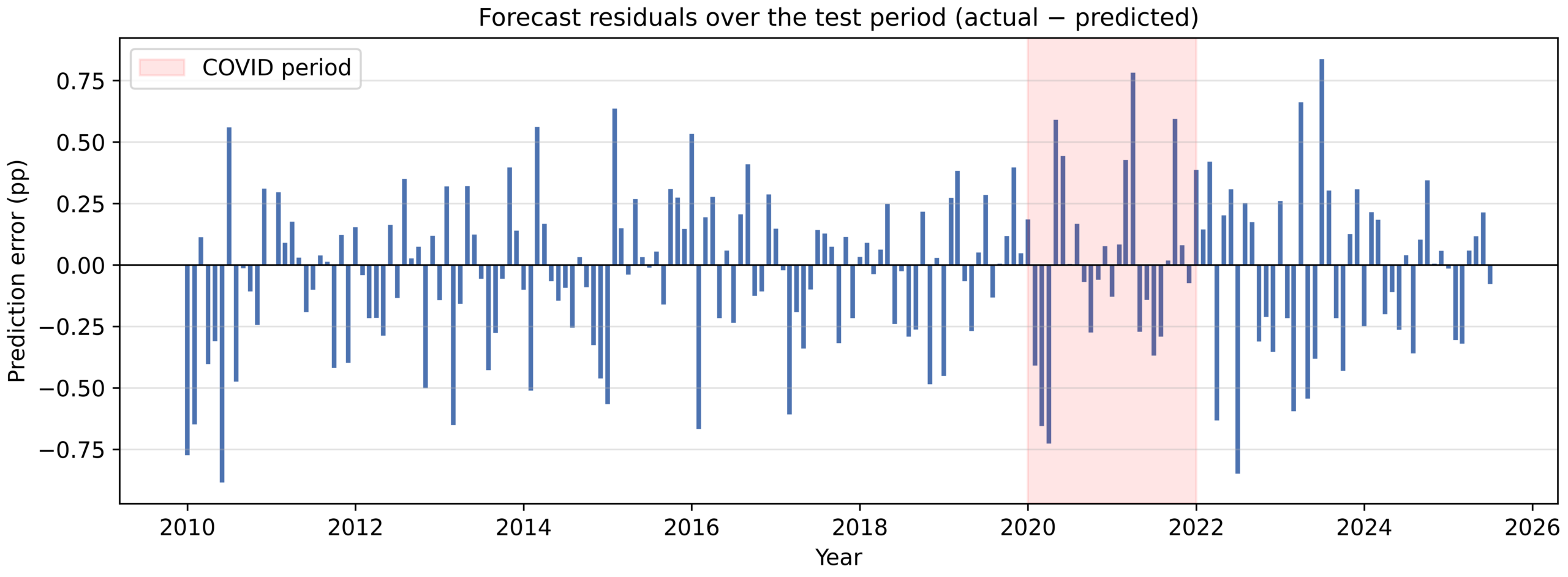
Sub-period R² values are not directly comparable across windows because R² depends on the variance of inflation within each window. Pre-COVID inflation was unusually stable, which lowers R² even though errors were smallest in that period, so RMSE and MAE are the more informative comparison. By those measures, forecast error rose by roughly 26% during 2020–2021 (RMSE 0.372 versus 0.296 percentage points pre-COVID) and remained slightly elevated afterward (0.349 pp). Figure 7 plots the individual forecast errors over time and shows that the largest misses cluster in 2020 and 2021 rather than being spread evenly across the test period.

Discussion

The results of this study show a strong historical co-movement between PPI and CPI. However, the baseline comparison in Table 2 indicates that this does not translate into predictive gains and the accuracy improvement from adding PPI to a model that already uses past CPI is not statistically distinguishable from zero, under either loss function and under both fixed-origin and expanding-window evaluation. While these results are informative, there are some limitations that prohibit further analysis.

Returning to the hypothesis stated in the introduction, that PPI is a leading predictor of CPI at a measurable time lag, the evidence supports it only partially. A leading relationship is statistically detectable. Both PPI lags are significant under HAC standard errors (p = 0.003 and p = 0.022) and BIC selects a short lag structure of two months, which is consistent with a genuine but brief lead. What the evidence does not support is the practical strength implied by the original framing. PPI alone cannot forecast CPI out of sample at all (Model B, R² = −0.56), and adding PPI to a model that already knows recent CPI produces an improvement of about 2% in RMSE that a formal test of equal predictive accuracy cannot distinguish from zero (p = 0.53). A statistically detectable in-sample lead and a useful out-of-sample forecasting gain are therefore not the same thing, and this study finds the first without the second. The hypothesis is therefore accepted in its weak form, that PPI leads CPI, and rejected in its strong form, that PPI is a reliable standalone predictor of CPI.

Identifying anomalies is important to keep in mind when looking at the price relationship between producers and consumers. Although changes in the relationship between PPI and CPI maintained a consistent correlation in the long term, there were several anomalies that were found, the biggest one being during the COVID-19 pandemic.

Within the COVID-19 pandemic, there were unanticipated effects on the relationship between producer and consumer price levels because of the dramatic shifts within the supply and demand of goods. Between January and March 2020, the CPI experienced a decline in market sectors that included but were not limited to transportation, lodging, and recreation. This decline was primarily caused by the collapse in consumer demand from the nationwide lockdown, travel restrictions, and uncertainty. However, producer prices did not fall proportionally to consumer prices as many firms faced fixed costs. This anomaly caused a temporary break in the usual relationship between PPI and CPI. My model, which assumes relatively stable patterns, struggled with the anomalies because consumer prices were more driven by pandemic shocks rather than producer prices.

As the COVID-19 pandemic continued, a large portion of the global supply chain was disrupted. In many cases, factories were closed and labor shortages caused increased product costs to be incurred by producers. However, producers did not have the ability to pass on these increased costs to consumers as consumers remained uncertain regarding how much they would spend. This created a period where producer prices rose without a corresponding increase in consumer prices. This observation was consistent with the findings from¹⁸.²⁸ quantify this channel directly, finding that exposure to global supply chain disruption was a significant driver of cross-industry US producer price inflation through 2021.

The COVID-19 pandemic presented unique challenges to the BLS in compiling the CPI. During Spring 2020, in-person data collection ceased almost overnight at brick-and-mortar stores and switched to online collection, increasing the rate of survey nonresponse and missing data in the CPI surveys. The April 2025 Article in the BLS’ Monthly Labor Review: Impacts of COVID-19 on collection and missing data in the CPI²⁹ mentions that to monitor the impacts of these issues on the CPI, BLS developed and began releasing new metrics each month. These new metrics show that the data collection disruptions caused by the COVID-19 pandemic were substantial, but in many cases the new metrics have returned to their pre-pandemic levels.

When the economy recovered in 2021 and 2022, the lag finally closed. Built up demand and a rapid proliferation in travel and consumer spending attributed to CPI’s sharp surge in 2022. Rather than reflecting a new inflation shock, this surge in consumer prices simply represented a delayed display of producer-level price increases that had begun earlier in the pandemic. This episode illustrates that the co-movement between the two series re-emerges once a disruption passes, although the sub-period results below show that the model’s accuracy was measurably worse while the disruption was under way.

The sub-period analysis in Table 4 quantifies this narrative and the model’s RMSE rises from 0.296 percentage points in the pre-COVID test years to 0.372 percentage points during 2020–2021, a roughly 26% increase in forecast error, before partially recovering after 2022. The disruption is therefore real but moderate in magnitude and even at its worst, the model’s typical error remained under half a percentage point.

Next, the data used in this study was limited to a monthly frequency, which limited my ability to analyze short term price shocks. Price and supply changes are dynamic on a day to day and week by week basis. Access to data sets which look at these more specific timetables, such as daily gasoline prices or weekly shipping rates, would allow more accurate estimates of the lagged predictions between PPI and CPI.

Another limitation of the study is the use of an aggregated measure of PPI and CPI. When examining price inflation on a broad basis, aggregate measures provide insight into patterns relating to price inflation and consumer pricing. However, on an individual basis, they do not provide an accurate representation of how price transmission occurs across individual markets. It does this primarily because the way in which price transmission occurs differs from industry to industry based on the interactions of supply chain factors within those industries, which results in producer price increases being transmitted to consumers at different rates by different industries.

For example, the transportation industry may experience a different response to higher fuel prices, shipping rates, and overhead costs, along with the timing of changes associated with those costs, as compared to other industries, including the timing of changes in overall economic conditions and the price of goods and services. Examining specific sectors will yield considerably more information on price transmission than looking at average measurements across industries. Doing so will enable a more precise determination of the amount of time it takes for price change shifts from producers to consumers in any given sector as compared to the average across all sectors.

This study deliberately uses only lagged PPI and lagged CPI as predictors and the exclusion of other known inflation drivers is a scope decision rather than an oversight. Exchange rate movements pass through to consumer prices with dynamics that differ substantially across countries and periods, monetary policy and commodity or supply-chain shocks operate through channels distinct from the producer-cost channel studied here^30,31, and household inflation expectations have been shown to shift the inflation process itself³². Adding these variables would turn the design into a general inflation-forecasting exercise such as that presented in the existing data-rich machine learning literature and would make it harder to isolate the specific question this paper asks, how much predictive information PPI adds beyond inflation’s own history. Extending the baseline comparison of Table 2 to these additional predictor blocks is a natural next step. Peer-reviewed evidence supports treating each of these as a distinct channel. Campa and Goldberg³³ document incomplete and country-varying exchange rate pass-through into import prices, and Ascari, Bonam and Smadu³⁴ find that global supply-chain pressure shocks have a persistent, hump-shaped effect on inflation that operates separately from the producer-cost channel studied here.

My study focuses on data prior to 2025; however, I note that in 2025, consumer prices rose slowly despite economists’ warnings that the current administration’s wide-ranging tariff agenda would increase costs for both U.S. businesses and consumers. That is partly because some importers took steps to offset the impact by preordering inventory and absorbing some tariffs to shield consumers in the short term. But because there were stop-gap measures, economists have warned consumers are unlikely to be insulated from tariff-driven inflation indefinitely. The latest PPI data underscores that higher prices are rippling through the economy, experts say.³⁵ note in their FEDS Notes that price pressures developed gradually in 2025 rather than showing up as a one-time spike and tariff effects have been greatest for goods imported from China with 8.5% year-over-year price increase by December 2025, and tariff pass-through to consumers between April and December 2025 has been at least 30% for goods imported from China. This gradual pattern is consistent with the peer-reviewed evidence from the 2018 tariff episode, in which³⁶ found near-complete pass-through of tariffs into US domestic prices, with the incidence falling on domestic importers and consumers.³⁷ reach a consistent conclusion using a real-time detection method, finding that the 2025 tariffs passed through partially to consumer goods prices within months of implementation.

Future Work and Ideas for Improvements

Future work on this topic could include evaluating my hypothesis to see if it applies universally and not just in the U.S. (i.e. comparing performance across the Americas, Europe, and China to see if PPI leads CPI over there).

Additional future work could include studying specific limitations of the linear ridge model used here. Regime-switching or time-varying-parameter models would allow the PPI–CPI relationship to change during disruptions such as COVID-19, which Table 4 shows is exactly when the model’s errors are largest. Recurrent neural networks such as LSTMs can capture nonlinear dynamics that a linear specification cannot²², and tree-based ensembles such as random forests handle much larger predictor sets and have delivered the largest documented gains in the U.S. inflation forecasting²⁰_. Though both approaches trade away the interpretability that motivated the present design. Applying the same baseline-controlled evaluation to sector-level price indices and to other countries would also test whether PPI’s weak incremental signal at the aggregate level masks stronger pass-through in specific industries or economies.

As mentioned in the BLS methodology report³⁸, there are key technical differences in how the CPI and the PPI indices are calculated by the BLS. CPI implements a geometric mean formula whereas PPI does not. Geometric calculation reduces substitution bias, leading to lower measures of inflation in periods of price increases. The PPI attempts to collect prices for a specific day of the month (the Tuesday of the week containing the 13th), while the CPI collects prices throughout the month. Finally, prices measured by the CPI include sales and excise taxes, while prices measured by the PPI exclude those taxes. Future improvement in the analyses presented in this paper could include studying these technical differences and incorporating them into the regression models.

Conclusion

This study finds that CPI YoY inflation can be forecast accurately one month ahead, but that most of this accuracy comes from the persistence of inflation itself rather than from producer prices. Adding lagged PPI to a CPI-only autoregressive baseline reduces out-of-sample RMSE by about 2%, an improvement that a Diebold–Mariano test cannot distinguish from zero (p = 0.53 under squared-error loss, p = 0.86 under absolute-error loss), with the same conclusion under expanding-window validation. Thus, although the PPI and CPI exhibit strong historical co-movement, this study does not find statistically significant evidence that PPI improves out-of-sample CPI forecasts once the information contained in past CPI is accounted for.

During the COVID-19 disruption of 2020–2021, the model’s RMSE increased from 0.296 percentage points in the pre-COVID period to 0.372 percentage points, an increase of approximately 26%. Forecast errors remained somewhat elevated after 2022. These results indicate that the historical relationships captured by the model became less reliable during the pandemic. While shifts in consumer demand, supply-chain disruptions, labor shortages, and other pandemic-related shocks offer possible explanations for this instability, the regression design used here does not identify the causal contribution of these individual factors.

The study also highlights several limitations. The use of monthly data restricts the ability to capture short-term price dynamics, while reliance on aggregate PPI and CPI measures obscures important sectoral differences in price transmission. Industry-specific factors, such as cost structures and supply chain dynamics, can strongly influence both the timing and magnitude of price pass-through, suggesting that disaggregated analysis would yield more precise insights.

Overall, the findings demonstrate that strong historical co-movement between PPI and CPI does not necessarily translate into meaningful out-of-sample forecasting gains. Lagged PPI contains statistically detectable information about CPI inflation in-sample, but once inflation’s own persistence is accounted for, its incremental improvement in out-of-sample forecast accuracy is small and not statistically distinguishable from zero. These results suggest that aggregate PPI should be viewed as a limited supplementary indicator of CPI inflation rather than a reliable standalone predictor.

Acknowledgements

I would like to acknowledge Dr. George Shakan, Applied Scientist at Amazon, for his support and guidance with this paper, including assistance with modeling and data analysis.

References

1. U.S. Bureau of Labor Statistics. Consumer Price Index for All Urban Consumers: All Items (CPIAUCSL) [Data set]. FRED, Federal Reserve Bank of St. Louis, 2025, https://fred.stlouisfed.org/series/CPIAUCSL. [↩] [↩]
2. U.S. Bureau of Labor Statistics. Producer Price Index by Commodity: All Commodities (PPIACO) [Data set]. FRED, Federal Reserve Bank of St. Louis, 2025, https://fred.stlouisfed.org/series/PPIACO. [↩] [↩]
3. S. Li, G. Tang, D. Yang, S. Du. Research on the relationship between CPI and PPI based on VEC model. Open Journal of Statistics, 9(2), pg. 218–229, 2019. [↩]
4. A. K. Tiwari, K. G. Suresh, M. Arouri, F.Teulon. Causality between consumer price and producer price: Evidence from Mexico. Economic Modelling, 36, pg. 432–440, 2014. [↩]
5. Y. Chen. Research on the relationship between PPI, enterprise commodity price index, M2 and CPI. Journal of Liaoning University (Philosophy and Social Sciences), 39, pg. 97–103, 2011. [↩]
6. G. Fan, L. He, J. Hu. CPI vs. PPI: Which drives which? Frontiers of Economics in China, 4(3), pg. 317–334, 2009. [↩] [↩]
7. W. K. Xu. On the consumer price index and producer price index: Who drives who? Questioning in a paper. Economic Research Journal, (5), pg. 139–148, 2010. [↩]
8. M. Shahbaz, R. U. Awan, M. Nasir. Producer and consumer prices nexus: ARDL bounds testing approach. International Journal of Marketing Studies, 1(2), pg. 78–86, 2009. [↩]
9. J. Sidaoui, C. Capistrán, D. Chiquiar, M. Ramos-Francia. A note on the predictive content of PPI over CPI inflation: The case of Mexico (Working Paper No. 2009-14). Banco de México, 2010. [↩]
10. Y.V. Topuz, H. Yazdifar, S. Sahadev. The relation between the producer and consumer price indices: A two-country study. Journal of Revenue and Pricing Management, 17(3), pg. 122–130, 2018. [↩]
11. A. K. Tiwari. An empirical investigation of causality between producers’ price and consumers’ price indices in Australia in frequency domain. Economic Modelling, 29(5), pg. 1571–1578, 2012. [↩]
12. J. Sun, J. Xu, X. Cheng, J. Miao, H. Mu. Dynamic causality between PPI and CPI in China: A rolling window bootstrap approach. International Journal of Finance & Economics, 28(2), pg. 1279–1289, 2023. [↩]
13. T. R. Aphane, C. L. Muchopa, M. P. Senyolo. Causality relationship between producer and consumer price indexes of selected meat commodities in South Africa from 1991 to 2023. Economies, V. 12(12), pg. 336, 2024. [↩]
14. T. E. Clark. Do producer prices lead consumer prices? Federal Reserve Bank of Kansas City Economic Review, 80(3), pg. 25–39, 1995. [↩]
15. G. M. Caporale, M. Katsimi, N. Pittis. Causality links between consumer and producer prices: Some empirical evidence. Southern Economic Journal, 68(3), pg. 703–711, 2002. [↩]
16. M. F. Ghazali, O. A. Yee, M. Z. Muhammad. Do producer prices cause consumer prices? Some empirical evidence. International Journal of Business and Management, 3(11), pg. 78–82, 2008. [↩]
17. S. Akçay. The causal relationship between producer price index and consumer price index: Empirical evidence from selected European countries. International Journal of Economics and Finance, 3(6), pg. 227–232, 2011. [↩]
18. J. Kasera, H. Powers. Using economic indicators to create an empirical model of inflation. Journal of Emerging Investigators, 2022, https://emerginginvestigators.org/articles/22-076. [↩] [↩]
19. J. H. Stock, M. W. Watson. Forecasting inflation. Journal of Monetary Economics, 44(2), pg. 293–335, 1999. [↩]
20. M. C. Medeiros, G. F. R. Vasconcelos, Á. Veiga, E. Zilberman. Forecasting inflation in a data-rich environment: The benefits of machine learning methods. Journal of Business & Economic Statistics, 39(1), pg. 98–119, 2021. [↩] [↩]
21. T. T. Nguyen, H. G. Nguyen, J. Y. Lee, Y. L. Wang, C. S. Tsai. The consumer price index prediction using machine learning approaches: Evidence from the United States. Heliyon, 9(10), e20730, 2023. [↩]
22. A. Almosova, N. Andresen. Nonlinear inflation forecasting with recurrent neural networks. Journal of Forecasting, 42(2), pg. 240–259, 2023. [↩] [↩]
23. F. X. Diebold, R. S. Mariano. Comparing predictive accuracy. Journal of Business & Economic Statistics, 13(3), pg. 253–263, 1995. [↩]
24. D. Harvey, S. Leybourne, P. Newbold. Testing the equality of prediction mean squared errors. International Journal of Forecasting, 13(2), pg. 281–291, 1997. [↩]
25. M. Jain. Perceived inflation persistence. Journal of Business & Economic Statistics, 37(1), pg. 110–120, 2019. [↩]
26. M. J. Beechey, P. Österholm. The rise and fall of U.S. inflation persistence. International Journal of Central Banking, 8(3), pg. 55–86, 2012. [↩]
27. W. K. Newey, K. D. Wes. A simple, positive semi-definite, heteroskedasticity and autocorrelation consistent covariance matrix. Econometrica, 55(3), pg. 703–708, 1987. [↩]
28. J. LaBelle, A. M. Santacreu. Global supply chain disruptions and inflation during the COVID-19 pandemic. Federal Reserve Bank of St. Louis Review, 104(2), pg. 78–91, 2022. [↩]
29. U.S. Bureau of Labor Statistics. Impacts of COVID-19 on collection and missing data in the Consumer Price Index. Monthly Labor Review, 2025, https://www.bls.gov/opub/mlr/2025/article/impacts-of-covid-19-on-collection-and-missing-data-in-the-cpi.htm. [↩]
30. M. V. Gordon, T. E. Clark. The impacts of supply chain disruptions on inflation (Economic Commentary No. 2023-08). Federal Reserve Bank of Cleveland, 2023. [↩]
31. D. A. Comin, R. C. Johnson, C. J. Jones. Supply chain constraints and inflation (NBER Working Paper No. 31179). National Bureau of Economic Research, 2023. [↩]
32. O. Coibion, Y. Gorodnichenko. Is the Phillips curve alive and well after all? Inflation expectations and the missing disinflation. American Economic Journal: Macroeconomics, 7(1), pg. 197–232, 2015. [↩]
33. J. M. Campa, L. S. Goldberg. Exchange rate pass-through into import prices. The Review of Economics and Statistics, 87(4), pg. 679–690, 2005. [↩]
34. G. Ascari, D. Bonam, A. Smadu. Global supply chain pressures, inflation, and implications for monetary policy. Journal of International Money and Finance, 142, 103029, 2024. [↩]
35. S. Hacioglu-Hoke, S. Malladi, L. Feler. The slow climb: How tariffs gradually raised retail prices in 2025. FEDS Notes. Board of Governors of the Federal Reserve System, 2026. [↩]
36. M. Amiti, S. J. Redding, D. E. Weinstein. The impact of the 2018 tariffs on prices and welfare. Journal of Economic Perspectives, 33(4), pg. 187–210, 2019. [↩]
37. R. Minton, M. Somale. Detecting tariff effects on consumer prices in real time. FEDS Notes. Board of Governors of the Federal Reserve System, 2025. [↩]
38. U.S. Bureau of Labor Statistics. How does the Producer Price Index differ from the Consumer Price Index? Comparing the personal consumption PPI with the CPI. BLS Methodology Report, 2023, https://www.bls.gov/ppi/methodology-reports/comparing-the-producer-price-index-for-personal-consumption-with-the-us-all-items-cpi-for-all-urban-consumers.html. [↩]