Enhancing Insights into Obesity and Health-Related Outcomes Using Regressions: A Study of the Carolinas

February 18, 2026

Abstract

Poor physical and mental health, obesity, and physical inactivity are major public health concerns in the United States, with profound implications for population well-being and health system burden. In this study, we focus on four key county-level health outcomes, physically unhealthy days, mentally unhealthy days, percentage of adults with obesity, andpercentage of physically inactive adults, to identify high-risk geographic regions and associated social determinants of health (SDOH). We integrate 300 county-level variables from theAgency for Healthcare Research and Quality’s (AHRQ) SDOH Database, along with health outcome data from the County Health Rankings & Roadmaps. Multiple predictive linear regression modeling approaches, including ordinary least squares (OLS) regression, Lasso regression for modeling each response separately, and group Lasso regression for joint modeling of four responses, were applied to forecast the following year’s values for each of the four outcomes. Model performance was evaluated using mean squared error, with Lasso and group Lasso regression achieving competitive results across outcomes compared to OLS regression. Key predictors include economic and social factors such as counties with a lower median home value of owner-occupied housing units and a higher percentage of family households with no spouse. The findings highlight specific geographic regions, such as inland rural areas, as areas of concern. These findings identify predictive associations that can guide hypothesis generation and preliminary policy discussions, while further causal analysis is needed before intervention.

Keywords: Behavioral and Social Sciences; County-Level Prediction; Mental and Physical Health Burden; Obesity; Physical Inactivity; Public Health

Introduction

Chronic physical and mental health burdens, such as obesity, physical inactivity, and poor self-reported health, remain among the most pressing public health challenges in the United States¹^,²^,³. Obesity alone is associated with increased risk for heart disease, diabetes, and certain cancers, contributing significantly to premature mortality and healthcare costs⁴^,⁵^,⁶. In parallel, physically and mentally unhealthy days, as well as insufficient physical activity, reflect broader well-being and functioning and are closely linked to underlying socioeconomic and environmental conditions⁷^,⁸.

These conditions are particularly concerning in the southeastern United States, where the prevalence of obesity and physical inactivity is often higher than the national average⁹^,¹⁰. For instance, in 2024, either South Carolina (SC) or North Carolina (NC) report elevated rates of obesity (36% in SC and 36% in NC versus the national average of 34%) and poor mental health (average numbers of mentally unhealthy days reported in past 30 days (age-adjusted) are 4.5 in NC and 5.4 in SC versus the national average of 4.8) and physical unhealth days (average numbers of physically unhealthy days reported in past 30 days (age-adjusted) are 3.3 in NC and 3.8 in SC versus national average of 3.3) compared to national benchmarks¹¹. These disparities underscore the urgent need for targeted, data-driven public health interventions.

It is documented that there are geographic variations in chronic disease burden (such as obesity¹², physical inactivity¹³, self-reported poor physical and mental health¹⁴). Based on Behavior Risk Factors Surveillance System data (BRFSS) 1995-2012, Dwyer-Lindgren et al. reported substantial geographic disparities in poor self-reported health (SRH) including self-reported general health, physical distress, mental distress, and activity limitation¹⁴. Another study used both BRFSS and National Health and Nutrition Examination Survey (NHANES) demonstrated an increase in the prevalence of sufficient physical activity from 2001 to 2009 which was matched by an increase in obesity in almost all counties during the same time period¹². During 1993–2001, BRFSS respondents in Alabama, Connecticut, Maine, New Jersey, New Mexico, North Carolina, and Oregon reported both increasing physically and mentally unhealthy days¹⁵. An overall worsening physical and mental health were reported from January 1993 to December 2006 using monthly observed mean physically and mentally unhealthy days from BRFSS¹⁶. A significant trend over time for increasing fair/poor SRH was found based on NHANES 2001–2016 data¹⁷. Robust association was reported between the social determinants of health (SDOH) and SRH¹⁸^,¹⁹^,²⁰.Scheinker, Valencia and Rodriguez found that county-level demographic, socioeconomic, health care, and environmental factors explain the majority of variation in county-level obesity prevalence²¹. Using 2000 BRFSS, Jia et al. indicated that socioeconomic variables predicted similar mean numbers of physical and mental unhealthy days at both the state and county level²².

To better address these issues, it is essential to understand the spatial and temporal patterns of these outcomes and the SDOH that contribute to them. However, dynamic, county-level analyses of such health indicators remain limited, particularly those leveraging comprehensive SDOH data.

This study aims to answer the following central question: “How can we dynamically predict county-level obesity, physical and mental health burden, and physical inactivity using SDOH data, and identify the most influential predictors?”

We use the Agency for Healthcare Research and Quality (AHRQ) SDOH Database, a publicly available, longitudinal resource that offers standardized county-level data across multiple domains of SDOH, including economic stability, education, healthcare access and quality, neighborhood environment, and community context²³. We integrate this dataset with health outcome measures from the County Health Rankings & Roadmaps to model and forecast county-level trends²⁴.

The key contributions of this study include:

Dynamic prediction of health outcomes using several linear regression methods, including ordinary least squares (OLS) regression, Lasso regression, and group Lasso regression;
Incorporation of comprehensive SDOH features (300 variables); and
Identification and interpretation of the most influential SDOH markers associated with each outcome.

Our work is novel in its integration of penalized regression and joint modeling of multiple outcomes combined with time-aware validation to enhance forecasting robustness. By identifying high-risk counties and critical social determinants, our findings can inform targeted public health strategies aimed at improving population health and reducing disparities.

Methods

To forecast next-year outcomes for county-level obesity, physical inactivity, and physically and mentally unhealthy days, we employed a suite of linear regression models: OLS regression, Lasso regression, and group Lasso regression using comprehensive SDOH predictors. Based on the County Health Rankings & Roadmaps database, the obesity is measured by percentage of adults that report BMI >= 30; physical inactivity is reported as percentage of adults that report no leisure-time physical activity; the physically unhealthy days is defined as average number of reported physically unhealthy days per month; and mental health unhealthy days is calculated by the average number of reported mentally unhealthy days per month. A comprehensive set of SDOH variables for counties in NC and SC were combined using the AHRQ SDOH Database. This curated resource integrates data from multiple federal and public datasets, including the American Community Survey (ACS), the Area Health Resources Files (AHRF), and the American Foundation for AIDS Research (AMFAR).

Data Processing

To ensure consistency and completeness across both states, we restricted our analysis to variables with no missing data across all counties in NC and SC. This filtering process resulted in a final set of 300 predictor variables. The majority of the variables (260) were sourced from ACS, capturing detailed demographic and socioeconomic information. An additional 27 variables representing healthcare provider characteristics were obtained from AHRF, while 13 variables describing healthcare facility attributes were drawn from AMFAR.

For modeling purposes, the positive physically and mentally unhealthy days variables were log-transformed with the following formula:

(1) $\begin{equation*}x \rightarrow \ln x.\end{equation*}$

The proportion-based outcomes were logit transformed using the following formula:

(2) $\begin{equation*}x \rightarrow \ln \frac{x}{100-x}.\end{equation*}$

These transformations convert the count or percentage outcome variables to a continuous scale on the real line without restriction, enabling more effective linear regression. Note that our dataset contains no zero counts and no percentages equal to 0 or 1, so the log transformation does not produce undefined values.

For the predictors, all 300 SDOH variables were standardized before analysis to place them on a common scale. Each variable was transformed to have a mean of zero and a standard deviation of one, ensuring comparability across features with different units and magnitudes. This preprocessing step prevents any single variable from disproportionately influencing the model due to its scale, which is particularly important when using regularization-based methods²⁵.

Procedures

To evaluate model performance, we used a year-based cross-validation framework in which each year from 2017 to 2021 was used for prediction evaluation while training was performed on all preceding years. The prediction error for each year was calculated using mean squared error (MSE), and we reported the average MSE across all folds for comparison.

To support the goal of forecasting future outcomes, we implemented a one-year temporal lag between predictors and response variables. For example, data from 2016 were used to predict health outcomes in 2017, data from 2017 to predict 2018 outcomes, and so on. This design mimics a real-world prediction scenario where only past and present information is available for future projections. We adopted a 3:1:1 temporal split of the data into training, validation, and test sets, respectively. That is, we trained the models using predictors from 2016–2018 with outcomes from 2017–2019, then validated on the next year (2019 predictors, 2020 outcomes) and tested on the following year (2020 predictors, 2021 outcomes). This allocation ensures sufficient data for model learning while preserving dedicated subsets for hyperparameter tuning and final model evaluation. Table 1 summarizes the datasets used across the modeling pipeline. The training set comprises three years of data from 146 counties (438 by 304 observations with 300 predictors and 4 outcomes). Each validation and prediction set uses one year of data, with 146 by 304 observations.

Stage	Sample Size	Predictors	Response
Training	438	SDOH Data from 2016-2018	Four health outcomes in 2017-2019
Validation	146	SDOH Data from 2019	Four health outcomes in 2020
Predictions	146	SDOH Data from 2020	Four health outcomes in 2021

Table 1 | Data used in each stage of modelling.

A major challenge in this framework is the limited sample size, especially for the training and validation sets. With only a few years of county-level data, statistical power to detect meaningful associations is reduced. This limitation also makes model calibration more difficult and increases the risk of overfitting, particularly in the context of the high-dimensional predictor space (300 SDOH features). Careful model selection and validation were therefore critical to mitigate instability in performance estimation. To prevent overfitting and make efficient use of the data, we employ a two-stage approach for methods requiring parameter tuning, including Lasso and group Lasso. Models are first trained on the training set, and tuning parameters are selected based on performance of the validation set. The final model is then refit using the combined training and validation data. For OLS regression, which does not require tuning, we fit the model directly on the combined training and validation set. Predictive performance is assessed on a separate test set.

Linear Regression

Linear regression models the relationship between a continuous outcome variable and one or more independent variables, under the assumption of a linear relationship²⁶. The model is expressed as:

(3) $\begin{equation*}y_i = \beta_0 + \sum_{j=1}^{p} \beta_j x_{ij} + \varepsilon_i,\end{equation*}$

where $\beta_0, \beta_1, \beta_2, \dots, \beta_p$ are the regression coefficients, $x_{i1}, x_{i2}, \dots, x_{ip}$ are the predictor variables and $\varepsilon_i$ is the error term in the $i$ -th county for $i=1,\dots,n$ .
The model is trained by minimizing the least squares cost function:

(4) $\begin{equation*}J(\beta) = \frac{1}{n} \sum_{i=1}^{n} \left( y_i - \beta_0 - \sum_{j=1}^{p} \beta_j x_{ij} \right)^2,\end{equation*}$

which measures the sum of squared differences between observed and predicted values.

Lasso Regression

Lasso regression builds upon linear regression by adding an L1 regularization term to the cost function²⁷^,²⁸.This penalizes the absolute values of the coefficients, encouraging sparsity in the model and enabling automatic variable selection. The Lasso cost function is:

(5) $\begin{equation*}J(\beta) = \frac{1}{n} \sum_{i=1}^{n} \left( y_i - \beta_0 - \sum_{j=1}^{p} \beta_j x_{ij} \right)^2 + \lambda \sum_{j=1}^{p} |\beta_j|,\end{equation*}$

where λ is the regularization parameter that controls the strength of the penalty. By shrinking less relevant coefficients toward zero, Lasso improves model interpretability and helps reduce overfitting.

To determine the optimal level of regularization, we implemented a hyperparameter tuning procedure that evaluated a range of λ values. For each value, we trained a Lasso model on the training set and evaluated its performance using MSE on a validation set. The model with the lowest validation MSE was selected as the best-performing Lasso model. In addition to overall prediction accuracy, we examined variable importance using the size of coefficients. Lasso selects a sparse set of predictors through penalized regression, enabling identification of key variables with strong linear associations.

Group Lasso Regression

The OLS regression and Lasso regression are applied separately to each response variable. While this approach is useful, it presents challenges for interpreting results across multiple responses. To address this and gain insights into predictors that influence all outcomes, we aim to jointly model the response variables and identify variables that are important across all four²⁹^,³⁰.Specifically, we estimate four regression models, one for each response, and treat the corresponding coefficients for each predictor as a group. The group Lasso penalty promotes group-wise sparsity: if a variable is unimportant for all responses, the entire group of coefficients is shrunk to zero. This encourages the selection of predictors that are jointly relevant, resulting in a more interpretable and effective model for our multivariate prediction task.

To further illustrate the idea, we use k to denote the k-th response variable. Then the model can be written as

(6) $\begin{equation*}y_{ik} = \beta_{0k} + \sum_{j=1}^{p} \beta_{jk} x_{ij} + \varepsilon_{ik},\end{equation*}$

where $\beta_{0k}, \beta_{1k}, \dots, \beta_{pk}$ are the regression coefficients for the $k$ -th response, $x_1, \dots, x_p$ are the predictor variables as before, and $\varepsilon_{ik}$ is the error term for the $k$ -th model for $k = 1, \dots, K$ . In our case, $K=4$ . Then, we apply the group Lasso regression for our problem. We define $p$ different groups for $p$ variables, each group of size $K$ corresponding to $K$ response variables. The group Lasso imposes an L2-norm for each group to impose groupwise sparsity. Thus, the corresponding objective function to minimize is:

(7) $\begin{multline*} J(\beta) = \frac{1}{n} \sum_{k=1}^{K} \sum_{i=1}^{n} \left( y_{ik} - \beta_{0k} - \sum_{j=1}^{p} \beta_{jk} x_{ij} \right)^2 + \lambda \sum_{j=1}^{p} \sqrt{\sum_{k=1}^{K} \beta_{jk}^2} \end{multline*}$

The joint linear model layout can be illustrated as follows:

(8) $\begin{equation*}\begin{bmatrix} X & 0 & 0 & 0 \\ 0 & X & 0 & 0 \\ 0 & 0 & X & 0 \\ 0 & 0 & 0 & X \end{bmatrix} \begin{bmatrix} \beta_1 \\ \beta_2 \\ \beta_3 \\ \beta_4 \end{bmatrix} + \begin{bmatrix} \varepsilon_1 \\ \varepsilon_2 \\ \varepsilon_3 \\ \varepsilon_4 \end{bmatrix} = \begin{bmatrix} y_1 \\ y_2 \\ y_3 \\ y_4 \end{bmatrix},\end{equation*}$

where $X$ is the n by p data matrix. Then the groups can be shown as

(9) $\begin{equation*}[\beta_1 \quad \beta_2 \quad \beta_3 \quad \beta_4] = \begin{bmatrix} \beta_{11} & \beta_{12} & \beta_{13} & \beta_{14} \\ \vdots & \vdots & \vdots & \vdots \\ \fbox{$\beta_{j1}$} & \fbox{$\beta_{j2}$} & \fbox{$\beta_{j3}$} & \fbox{$\beta_{j4}$} \\ \vdots & \vdots & \vdots & \vdots \\ \beta_{p1} & \beta_{p2} & \beta_{p3} & \beta_{p4} \end{bmatrix}.\end{equation*}$

Once the group Lasso solution is obtained, we identify the nonzero groups for the final selected set of predictors.

Trend Analysis and Visualization

We used pie charts, pairwise matrix plots, scatterplots, bar charts, and heatmaps to examine distributions, correlations, and spatiotemporal patterns across the four outcomes and to summarize prediction results.

To assess relationships among outcomes, we built a pairwise matrix: diagonal panels show each outcome’s marginal distribution (bar charts), and off-diagonal panels show pairwise scatterplots with overlaid Pearson correlations to quantify association strength and direction.

To characterize spatial patterns, we generated geographic heatmaps for each year, mapping county values to a color scale (darker = higher). Sequencing yearly heatmaps enabled visual comparison of regional variability and temporal change. After model selection, we applied the same heatmap approach to highlight important predictors across counties and to compare observed versus model-predicted outcomes.

Results

Figure 1 presents the distribution of 300 SDOH variables across 14 topics. Demographics accounts for the largest share, followed by housing and health insurance, underscoring the central role of structural and social factors in shaping population health outcomes. A breakdown of the 300 variables by data source is provided in the Supplementary file. Demographics comprised 94 variables, capturing population structure such as age and household composition. Housing (34 variables) and health insurance status (33 variables) reflected affordability, housing characteristics, and insurance coverage types. Employment (29 variables) and poverty (23 variables) described labor force participation and income relative to federal poverty thresholds. Measures of healthcare access included healthcare providers (14 variables) and healthcare facilities (13 variables), while income (14 variables) captured economic resources and inequality. Transportation, living conditions, and educational attainment each included 10 variables, reflecting commuting patterns, family structure, and educational levels. Smaller categories included immigration (9 variables), disability (4 variables), and migration (3 variables), capturing citizenship status, disability prevalence, and residential mobility.

Figure 1 | Pie chart of the 300 selected SDoH predictor variables by 14 topics.

We analyzed four county-level health outcomes from the County Health Rankings and Roadmaps dataset: the average number of physically unhealthy days reported per month, the average of mentally unhealthy days reported per month, the percentage of adults classified as obese, and the percentage reporting physical inactivity. To explore the relationships among these outcomes, we present a matrix of pairwise scatterplots for the 2017 data in Figure 2. The patterns for other years are similar and not included here. The plots reveal relatively strong linear associations, with correlation coefficients of at least 0.6. This aligns well with intuition: higher numbers of physically and mentally unhealthy days, along with higher rates of physical inactivity, are naturally associated with higher obesity prevalence. These findings underscore the value and relevance of jointly modeling the four outcomes.

Figure 2 | Matrix scatterplots among four outcome variables for the year 2017. The diagonal panels show histograms of the four outcomes (x-axis: variable range; y-axis: frequency).
The off-diagonal panels show pairwise scatterplots of the outcomes, with the Pearson correlation and the best-fit linear regression line overlaid (x-axis and y-axis represents two predictors with their range). Physically unhealthy days: the average number of physically unhealthy days reported per month; Mentally unhealthy days: the average of mentally unhealthy days reported per month, % obese: the percentage of adults classified as obese in percent, and % Physically inactive: the percentage reporting physical inactivity in percent.

To examine outcome trends, we present the average outcome values over time (2017-2021) for the top 10 counties in terms of each outcome in 2017 in Figure 3. Note, all outcomes are expressed as population-normalized measures (averages or percentages), thereby minimizing sensitivity to county population size. While some fluctuations are observed, the overall patterns show a steady increase over the years for outcomes of Mentally Unhealthy Days and % of Obesity. For example, % of obesity in Fairfield and Chester counties has a clear increasing trend during 2018-2021.

Figure 3 | Trends for the average four outcomes for top 10 counties in terms of 2017 ranking during 2017-2021.

Figures 4-7 present county-level heatmaps of four outcomes. The heatmaps reveal consistent spatial patterns across years and an overall worsening trend over time. To further characterize temporal patterns, we quantified the consistency of changes over time for each outcome by counting (i) counties exhibiting a strictly monotonic increase across all four years and (ii) counties showing increases in three of the four years. For obesity prevalence, 35 counties demonstrated monotonic increases, and 56 increased in three of four years. Physical inactivity showed fewer strictly monotonic increases (16 counties), though 70 counties increased in three of four years. No counties exhibited strictly monotonic increases in either physically unhealthy days or mentally unhealthy days; however, 13 and 74 counties, respectively, showed increases in three of the four years. York County has demonstrated the consistent increase in both obese and physical inactivity. Edgefield, Lee, and Macon Counties show a consistent increasing pattern in three of the four years across all four outcomes. 19 counties have consistent increasing pattern in three of the four years among three outcomes.

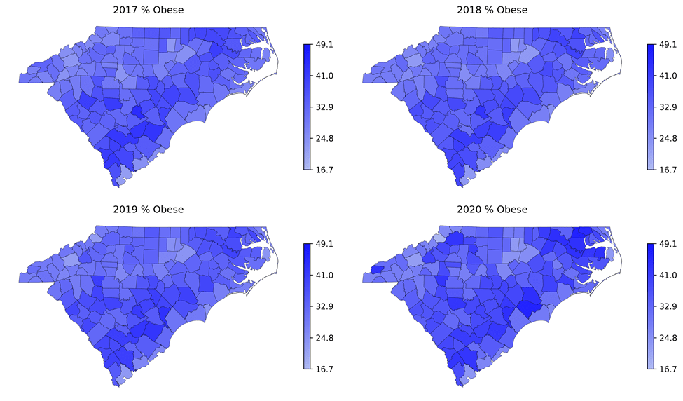
Figure 4 | Color maps for % of obesity in Carolinas during 2017-2020

Figure 6 | Color maps for mentally unhealthy days in Carolinas during 2017-2020

Table 2 reports the prediction accuracy for the four outcomes in 2021. Across all outcomes, transformed predictors consistently yield substantially lower MSEs than untransformed predictors, indicating improved model performance after transformation. Among the three modeling approaches, except mental unhealthy days, Lasso generally produces the lowest MSE for transformed predictors, followed by Group Lasso, and OLS gives the worst performance though differences between OLS and Group Lasso are relatively small for obesity. Interestingly, OLS tends to perform slightly worse than the penalized methods after transformation, although it works the best for the outcome of mental unhealthy days.

Although Lasso often achieved the lowest MSE among transformed predictors, group Lasso was chosen for subsequent analyses because it allows for structured feature selection by groups of related predictors, improving interpretability and aligning with the substantive domains of social determinants of health. This approach facilitates more meaningful recommendations for policy and intervention, as results can be interpreted at the domain level rather than focusing solely on individual covariates.

Outcome		OLS	Lasso	Group Lasso
Obesity	Transformed	0.04507	0.02914	0.04417
Obesity	Untransformed	23.12098	14.72717	22.73726
Physically unhealthy	Transformed	0.01762	0.01047	0.01680
Physically unhealthy	Untransformed	0.35889	0.20727	0.29761
Mentally unhealthy	Transformed	0.01690	0.02842	0.02940
Mentally unhealthy	Untransformed	0.34858	0.57479	0.58746
Physically Inactive	Transformed	0.04683	0.02865	0.03436
Physically Inactive	Untransformed	17.83918	11.31083	13.89089

Table 2 | Prediction accuracy for four outcomes based on three regression models: OLS, Lasso and group Lasso.

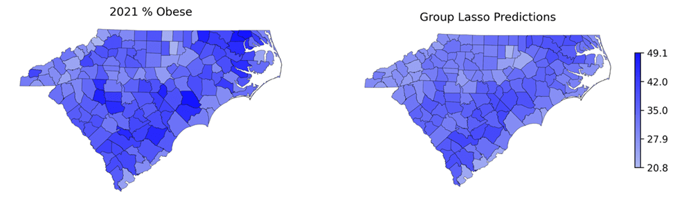
We further demonstrate the most important features based on the group lasso approach. In particular, we calculate the group norm for each variable, i.e., $\sqrt{\sum_{k=1}^K \beta_{jk}^2}$ for variable $j$ and then sort them. Figure 8 presents the top 10 most important variables using the group norm, including factors such as the median home value of owner-occupied housing units. These factors are most associated with the four outcomes. To further understand the direction of associations for each factor with the outcomes, Figure 9 shows heatmaps of the most important predictors and corresponding outcomes for the top 5 (right 5 columns) and bottom 5 counties (left 5 columns) sorted by the average outcomes. The results indicate that counties with higher median home values tend to have lower obesity rates, lower percentages of physical inactivity, and fewer mentally and physically unhealthy days. In contrast, higher percentages of family households without a spouse are associated with higher obesity rates and greater numbers of unhealthy days. Finally, Figure 10 maps the true and predicted outcomes for 2021, showing that the predictions capture spatial patterns well. However, the predicted heatmaps are generally lighter than the observed ones, suggesting underestimation. Two factors may contribute: (1) ongoing worsening of these outcomes over time that the models do not fully capture, and (2) limited sample size, which constrains predictive accuracy.

Figure 8 | Top predictors sorted by the group norm of coefficients by group Lasso

Figure 9 | Heatmap of top 5 and bottom 5 counties by outcome variables and the 5 most important factors. Darker (lighter) colors indicate higher (lower) values.

Figure 10 | True and predicted values for four outcomes in 2021.

Discussion

This study demonstrates the value of integrating comprehensive SDOH data with advanced regression‐based modeling to forecast county-level health outcomes: obesity, physical and mental health burden, and physical inactivity. Using the AHRQ SDOH Database with outcome measures from County Health Rankings & Roadmaps, we compared OLS, Lasso, and Group Lasso on both raw and transformed predictors. Preprocessing transformations substantially improved accuracy, especially for outcomes with wide variation in scale. Penalized methods generally work well. Among the methods, Group Lasso was selected for subsequent analyses because it performs structured feature selection at the domain level. This is well suited to county-level inference, where SDOH variables cluster naturally into domains (e.g., socioeconomic status, health-care access, built environment). Group-level selection enhances interpretability by highlighting the collective contribution of domains rather than isolated variables, which in turn supports clearer communication and more actionable, domain-targeted policy recommendations³¹.

Beyond model performance, incorporating 300 SDOH variables provided a richer view of socioeconomic, environmental, and community factors associated with adverse outcomes. The combination of high-dimensional, longitudinal data and penalized regression offers a scalable framework for flagging high-risk counties and supporting dynamic public-health surveillance to inform equity-focused planning. The selected predictors should be interpreted as predictive correlates, not necessarily causal drivers³²; policy implications should not be drawn from these associations without additional causal analysis that addresses confounding, measurement error, and other potential biases.

Conclusion

Our study combines the AHRQ SDOH Database with outcome measures from County Health Rankings & Roadmaps and applies OLS, Lasso, and Group Lasso regression. We find that transforming predictors and using penalized methods, especially Group Lasso, provides reasonable out-of-sample prediction of county-level health outcomes and highlights domain-level associations that can guide further investigation and, with appropriate caution, inform policy and intervention planning.

Acknowledgements

The authors would like to thank Dr. Peiyin Hung at the University of South Carolina for mentoring, the helpful comments and suggestions from the review team, the AHRQ for developing the AHRQ SDoH Database, and the University of Wisconsin Population Health Institute for County Health Ranking & Roadmaps data, and for making them available for public use.

References

D. R. Brown, D. D. Carroll, L. M. Workman, S. A. Carlson, D. W. Brown. Physical activity and health-related quality of life: US adults with and without limitations. Quality of life research, Vol. 23(10), pg. 2673-2680, 2014, https://doi.org/10.1007/s11136-014-0739-z [↩]
M. Bayliss, R. Rendas-Baum, M. K. White, M. Maruish, J. Bjorner, S. L. Tunis. Health-related quality of life (HRQL) for individuals with self-reported chronic physical and/or mental health conditions: panel survey of an adult sample in the United States. Health and quality of life outcomes, Vol. 10(1), pg. 154, 2012, https://doi.org/10.1186/1477-7525-10-154 [↩]
E. Robinson, A. Haynes, A. Sutin, M. Daly. Self‐perception of overweight and obesity: A review of mental and physical health outcomes. Obesity science & practice, Vol. 6(5), pg. 552-561, 2020, https://doi.org/10.1002/osp4.424 [↩]
G. A. Bray. Risks of obesity. Endocrinology and Metabolism Clinics, Vol. 32(4), pg. 787-804, 2003, https://doi.org/10.1016/S0889-8529(03)00067-7 [↩]
S. Sarma, S. Sockalingam, S. Dash. Obesity as a multisystem disease: Trends in obesity rates and obesity‐related complications. Diabetes, Obesity and Metabolism, Vol. 23, pg. 3-16, 2021, https://doi.org/10.1111/dom.14290 [↩]
D. Mohajan, H. K. Mohajan. Obesity and its related diseases: a new escalating alarming in global health. Journal of Innovations in Medical Research, Vol. 2(3), pg. 12-23, 2023, https://www.paradigmpress.org/jimr/article/view/505 [↩]
H. Jia, D. G. Moriarty, N. Kanarek. County-level social environment determinants of health-related quality of life among US adults: a multilevel analysis. Journal of community health, Vol. 34(5), pg. 430-439, 2009, https://doi.org/10.1007/s10900-009-9173-5 [↩]
K. C. McNamara, E. T. Rudy, J. Rogers, Z. N. Goldberg, H. S. Friedman, P. Navaratnam, D. B. Nash. The cost of unhealthy days: A new value assessment. Population Health Management, Vol. 27(5), pg. 307-311, 2024, https://doi.org/10.1089/pop.2024.0102 [↩]
D. F. Terrell. Overweight and obesity prevalence rates among youth in the Carolinas. North Carolina Medical Journal, Vol. 63(6), pg. 281-286, 2002, https://www.ncbi.nlm.nih.gov/pubmed/12970974 [↩]
D. G. Moriarty, M. M. Zack, R. Kobau. The Centers for Disease Control and Prevention’s Healthy Days Measures–Population tracking of perceived physical and mental health over time. Health and quality of life outcomes, Vol. 1(1), pg. 37, 2003, https://doi.org/10.1186/1477-7525-1-37 [↩]
University of Wisconsin Population Health Institute. (2024). Compare Counties. University of Wisconsin Population Health Institute. Retrieved Dec 25 from https://www.countyhealthrankings.org/health-data/compare-counties?year=2024&compareCounties=37000%2C45000%2C00000 [↩]
N. C. Black. An ecological approach to understanding adult obesity prevalence in the United States: a county-level analysis using geographically weighted regression. Applied Spatial Analysis and Policy, Vol. 7(3), pg. 283-299, 2014, https://doi.org/10.1007/s12061-014-9108-0 [↩] [↩]
R. An, X. Li, N. Jiang. Geographical variations in the environmental determinants of physical inactivity among US adults. International journal of environmental research and public health, Vol. 14(11), pg. 1326, 2017, https://doi.org/10.3390/ijerph14111326 [↩]
L. Dwyer-Lindgren, J. P. Mackenbach, F. J. van Lenthe, A. H. Mokdad. Self-reported general health, physical distress, mental distress, and activity limitation by US county, 1995-2012. Population health metrics, Vol. 15(1), pg. 16, 2017, https://doi.org/10.1186/s12963-017-0133-5 [↩] [↩]
H. S. Zahran, R. Kobau, D. G. Moriarty, M. M. Zack, J. Holt, R. Donehoo, C. f. D. Control, Prevention. Health-related quality of life surveillance—United States, 1993–2002. MMWR Surveill Summ, Vol. 54(4), pg. 1-35, 2005, https://www.ncbi.nlm.nih.gov/pubmed/16251867 [↩]
H. Jia, E. I. Lubetkin. Time trends and seasonal patterns of health-related quality of life among US adults. Public Health Reports, Vol. 124(5), pg. 692-701, 2009, https://doi.org/10.1177/003335490912400511 [↩]
M. L. Greaney, S. A. Cohen, B. J. Blissmer, J. E. Earp, F. Xu. Age-specific trends in health-related quality of life among US adults: Findings from National Health and Nutrition Examination Survey, 2001–2016. Quality of life research, Vol. 28(12), pg. 3249-3257, 2019, https://doi.org/10.1007/s11136-019-02280-z [↩]
H. Jia, D. G. Moriarty, N. Kanarek. County-level social environment determinants of health-related quality of life among US adults: a multilevel analysis. Journal of community [↩]
K. Wind, B. Poland, F. HakemZadeh, S. Jackson, G. Tomlinson, A. Jadad. Using self-reported health as a social determinants of health outcome: a scoping review of reviews. Health Promotion International, Vol. 38(6), pg. daad165, 2023, https://doi.org/10.1093/heapro/daad165 [↩]
C. Delpierre, V. Lauwers-Cances, G. D. Datta, T. Lang, L. Berkman. Using self-rated health for analysing social inequalities in health: a risk for underestimating the gap between socioeconomic groups? Journal of Epidemiology & Community Health, Vol. 63(6), pg. 426-432, 2009, https://doi.org/10.1136/jech.2008.080085 [↩]
D. Scheinker, A. Valencia, F. Rodriguez. Identification of factors associated with variation in US county-level obesity prevalence rates using epidemiologic vs machine learning models. JAMA Network open, Vol. 2(4), pg. e192884-e192884, 2019, https://doi.org/10.1001/jamanetworkopen.2019.2884 [↩]
H. Jia, P. Muennig, E. Lubetkin, M. R. Gold. Predicting geographical variations in behavioural risk factors: an analysis of physical and mental healthy days. Journal of Epidemiology & Community Health, Vol. 58(2), pg. 150-155, 2004, https://doi.org/10.1136/jech.58.2.150 [↩]
U.S. Department of Health and Human Services. Social Determinants of Health Database. Retrieved April 25 from https://www.ahrq.gov/sdoh/data-analytics/sdoh-data.html [↩]
University of Wisconsin Population Health Institute. County Health Rankings & Roadmaps, Health Data. . Retrieved April 25 from https://www.countyhealthrankings.org/health-data [↩]
J. M. H. Pinheiro, S. V. B. de Oliveira, T. H. S. Silva, P. A. R. Saraiva, E. F. de Souza, R. V. Godoy, L. A. Ambrosio, M. Becker. The Impact of Feature Scaling In Machine Learning: Effects on Regression and Classification Tasks. ArarXiv preprint, Vol., pg., 2025, https://doi.org/10.48550/arXiv.2506.0827 [↩]
S. Chatterjee, A. S. Hadi. (2015). Regression analysis by example. John Wiley & Sons. https://doi.org/10.1111/insr.12020_2 [↩]
J. Ranstam, J. A. Cook. LASSO regression. Journal of British Surgery, Vol. 105(10), pg. 1348-1348, 2018, https://doi.org/10.1002/bjs.10895 [↩]
R. Tibshirani. Regression shrinkage and selection via the lasso. Journal of the Royal Statistical Society Series B: Statistical Methodology, Vol. 58(1), pg. 267-288, 1996, https://doi.org/10.1111/j.2517-6161.1996.tb02080.x [↩]
M. F. Duarte, W. U. Bajwa, R. Calderbank. (2011). The performance of group Lasso for linear regression of grouped variables (Duke University, Dept. Computer Science, Durham, NC, Technical Report TR-2010-10). [↩]
M. Yuan, Y. Lin. Model selection and estimation in regression with grouped variables. Journal of the Royal Statistical Society Series B: Statistical Methodology, Vol. 68(1), pg. 49-67, 2006, https://doi.org/10.1111/j.1467-9868.2005.00532.x [↩]
H. Ohanyan, L. Portengen, A. Huss, E. Traini, J. W. Beulens, G. Hoek, J. Lakerveld, R. Vermeulen. Machine learning approaches to characterize the obesogenic urban exposome. Environment international, Vol. 158, pg. 107015, 2022, https://doi.org/10.1016/j.envint.2021.107015 [↩]
N. Altman, M. Krzywinski. Points of Significance: Association, correlation and causation. Nature methods, Vol. 12(10), pg. 899, 2015, https://doi.org/10.1038/nmeth.3587 [↩]

Enhancing Insights into Obesity and Health-Related Outcomes Using Regressions: A Study of the Carolinas

Abstract

Introduction