Detection and Characterization of Exoplanet Transits in Kepler Light Curves

Abstract

A large number of exoplanets have been discovered using the Box-Least Squares (BLS) algorithm, which fits periodic box-shaped models to light curve data to identify transiting exoplanets. This paper quantitatively analyzes the accuracy with which planetary characteristics can be inferred, specifically by estimating the uncertainty in the planet-to-star radius ratio. Evaluation is conducted by implementing a BLS algorithm to detect transit signals while acquiring, preprocessing, and visualizing Kepler light curve data. The study relies on light curves from the NASA Exoplanet Archive’s Kepler database, from which the algorithm successfully identifies a transit. Key parameters are inferred, allowing the retrieval of a precise ratio with a deviation of less than 1%. The corresponding uncertainty is then calculated, demonstrating that BLS is effective for estimating transit parameters with high precision under appropriate data conditions.

Keywords: exoplanet detection, transits, box-least squares, kepler light curves, periodogram analysis

Introduction

Exoplanets, planets located beyond our solar system, are a significant part of current studies in astrophysical research. Even though the planets discovered are within a relatively small part of our universe, specifically the Milky Way, they tend to be located at a distance of thousands of light years away from us. As a result, to classify them, parameters such as mass, temperature, chemical composition, and orbital characteristics are used with major categories including: gas giant, Neptunian, super-Earth, and terrestrial. Our data to classify them relies heavily on the method of detection, hence arises a need for indirect observational techniques.

Detection of exoplanets from Earth via direct observation remains difficult for us due to the vast distances, brightness contrast, and angular resolution. While direct imaging is occasionally used, to overcome these limitations, many observational techniques have been developed. Effective methods include radial velocity, the transit method, and gravitational microlensing. We can detect planets by using the radial velocity method, which, via measuring the periodic Doppler shifts caused by the star’s motion around a shared center of mass between the star and the planet, allows us to infer the presence of orbiting planets. However, it requires a high signal-to-noise ratio spectra for obtaining high precision, and additionally can only estimate a planet’s minimum mass due to unknown orbital inclination. It is a preferred method for low-mass and nearby planets, but due to these limitations, it is not well-suited for large photometric surveys. The transit method is preferred in such instances, as it allows efficient detection across light-curve datasets and measures planetary radii directly¹. However, planets with high orbital obliqueness will not produce observable transits. Gravitational microlensing depends on the bending of the gravitational field of a nearby star when it passes in front of a distant star. Due to the light being observed getting bent, the distant star looks brighter for a short amount of time. By contrast, it is the transit method that has yielded the largest number of exoplanet discoveries to date, and it forms the foundation of the present analysis.

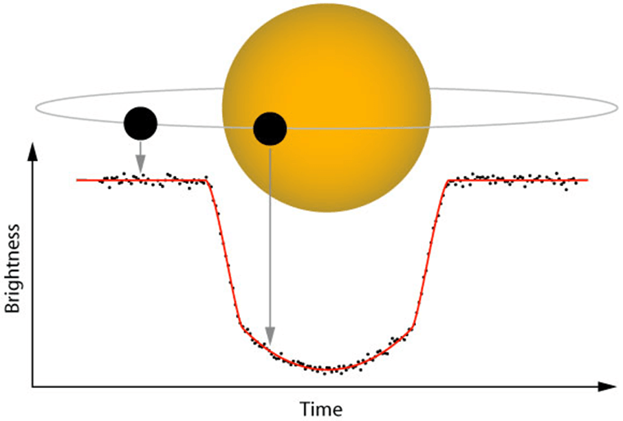
A temporary and periodic dip in the observed brightness occurs when planets pass in front of their host stars. This phenomenon is known as transit¹, forming the basis of the transit method. By graphing this characteristic variation in light from the host star, a light curve is obtained.

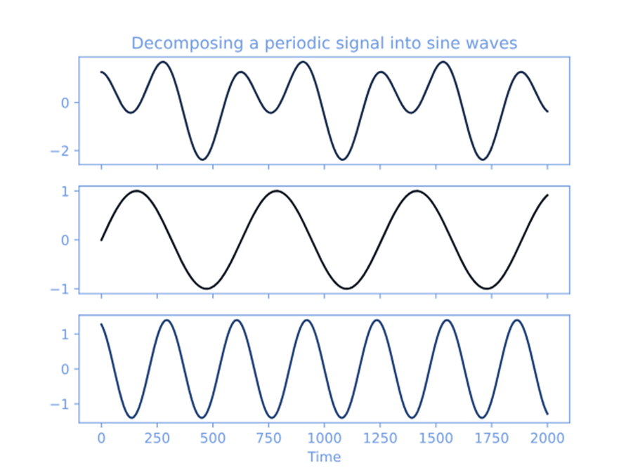
From this, a key planetary characteristic can be inferred: transits allow us to determine the orbital period of the planet. Such meaningful information can be acquired using various methods, including the Fourier transform^2,3 and Phase Dispersion Minimization^4,5. For added context, the Fourier transform is a mathematical method that utilizes light curve data by decomposing it into sine and cosine functions, thereby identifying repeating or periodic signals. It is used to detect variations such as those arising in pulsating stars and binary systems; thus is better suited for smooth sinusoidal signals as compared to box-shaped ones. When approximating nearly rectangular transit signals, Fourier methods need to include a large number of harmonics (7-10 or more) to closely resemble the shape of the transit, thus proving it to be suboptimal⁶.

Additionally, Phase Dispersion Minimization (PDM) is an algorithm that, unlike the Fourier transform, does not assume a sinusoidal shape. It analyzes the time-domain data by aligning observations over a range of trial periods and then evaluates the dispersion of flux using phase bins.  It was widely popular in the earlier times because the algorithm did not require computing trigonometric functions, as doing so would put a heavy load on the computers. Though this characteristic feature made it computationally attractive back in the day, it is not very well suited for detecting such rectangular signals. It produces broader transitions between noise and signal and can result in lower detection strength for sharp, periodic dips, adding to its disadvantages while evaluating transit signals⁶.

The limitations discussed above proved insufficient for detecting exoplanets. As such, a more specialized algorithm, that is, the Box Least Squares (BLS) algorithm, was developed, intending to rectify poor performance in relation to short-duration, box-shaped signals. The BLS algorithm is regarded as more effective than the above-mentioned methods. Unlike PDM and DFT, it is programmed to directly fit box-shaped dips, proving better efficient for non-sinusoidal events^6,7,8 and is particularly useful in conditions of especially noisy data, while also being more efficient and statistically powerful because of its model based approach.  

The BLS method, as stated above, primarily functions as a detection tool for identifying periodic signals in the light curves of stars, which can indicate the presence of a planet transiting in front of them, using a technique known as the transit method. After detecting a period, a light curve is constructed by organizing photometric data based on that detection period by “folding” the data over itself. This process results in a folded light curve. This light curve helps visualize repeating brightness variations, which makes it easier to study. Researchers then analyze the folded light curve to extract properties such as transit depth and duration, key indicators of the planet’s size and orbit, and the star’s brightness. This step is crucial for understanding both the star and the planet.  The BLS method, though, has added advantages over the other previously mentioned methods. The algorithm specifically relies on a predetermined box shape of the periodic light curve, manifesting in the high efficiency of this method in detecting true signals as compared to the other search methods (which are generic and tend to detect any periodic variation⁶. The strength of the algorithm’s detection relies primarily on the effective signal-to-noise ratio. The signal refers to how much the star’s brightness drops, while the noise comes from measurement errors and natural fluctuations of the star’s brightness. The signal-to-noise ratio needs to be greater than six, acting as a minimum to detect a transit confidently. This serves as an important factor when planning future searches for extrasolar planetary transits⁶.

Missions like Kepler (2009–2018) and its extended K2 campaign used transit photometry to detect over 2 600 confirmed exoplanets (NASA Exoplanet Archive, 2024), while TESS (Transiting Exoplanet Survey Satellite, launched in 2018) continues to identify planets orbiting nearby bright stars (NASA Exoplanet Archive, 2024). As of now, 4 381 exoplanets have been confirmed using the transit method. Upcoming missions, such as PLATO 2.0, will utilize transit photometry to detect and characterize planets⁹. Another notable mission, CHEOPS, is recognized as the first mission dedicated to searching for transits of exoplanets using ultrahigh precision photometry on bright stars, which involves using the transit method¹⁰.

The transit method, as mentioned earlier, helps detect exoplanets by observing repeated dips in brightness over time, which aids in identifying pivotal characteristics of planets¹. Detecting periodic transits is important for evaluating the existence of planets, and while being used broadly, difficulties remain in determining how accurately planetary parameters can be inferred^1,11. Hence, the primary aim of this study is to evaluate quantitatively the performance of the BLS method, which analyzes light curves to identify periodic signals using Kepler light curve data. The secondary aim of the study is to specify the uncertainty inferred from the planet to star radius ratio, crucial for later calculations. Finally, the analysis of educational reproducibility in relation to simplicity is evaluated, assessing whether reliable results can still be achieved without complex pipelines.

In Section 2, we explore the methodology and data used. Explanations for the light curve data, taken from NASA’s MAST archive, processes involved whilst implementing the BLS algorithm and tools for implementation, namely, Jupyter notebooks, and Numpy, have been given in the following segment, along with evaluation of detections and uncertainties.

Methods

This study utilizes an observational and cross-sectional approach, from which it observes existing archival data taken from the Kepler Mission for evaluating the BLS method. It involves running a custom implementation of the BLS algorithm, which relies solely on observational data. The main premise of the paper is to analyze such snapshots in astronomical time-series data to evaluate the ability to identify periodic transit signals, as output by the algorithm. Unlike other tools and packages that only outline the logic behind BLS’s operation, this study focuses on two aspects: coding the detection mechanism and examining how different inferred parameters affect the estimation of uncertainty in the inferred planet-to-star ratio. This is done to better understand the algorithm’s behavior when approached with real astronomical data, and makes it more reproducible. Additionally, implementation details are described explicitly to support reproducibility for educational purposes. Residual analysis is performed to draw differences between the paper’s manual implementations and SciPy’s built-in functions for better evaluation. This makes it easier to understand how each parameter would affect the results. Preprocessing steps are done to prepare the light curve, followed by a Box-Least-Squares program. From this, we can, in future studies, adjust the model to refine performance realistically. The analysis of the BLS method is, hence, significant to understanding the practical behaviour and limitations under realistic observation.

Data: Kepler Q1 Long-Cadence SAP Light Curve (KIC 11904151)

The Kepler Mission serves as a very significant tool for our understanding of the universe. Launched on March 6, 2009, it performed photometric surveys of more than 100 000 dwarf stars to search for terrestrial-sized planets, using the transit technique, though designed mainly to detect Earth-size planets in the habitable zone– regions with conditions suitable for the existence of water around solar-like stars. From the commissioning and quarter 1 (Q1) data sets, 177 Kepler targets had been identified as “Kepler Objects of Interest”. An additional 100 000 late-type dwarf stars, with visual magnitudes between 9 and 16, were also surveyed for 3.5 years¹². This was to look for transits of planets around those stars. Owing to Kepler’s ability to analyze exact brightness measurements taken continuously over a long time, its data has proved very valuable for discovering exoplanets.

For this study, observational sample data from the Kepler Mission are analyzed, and obtained via the Mikulski Archive for Space Telescopes (MAST). With intervals sampled at approximately 29.4 minutes, evaluation of its long cadence light curve data is done for the target of Kepler-10b (KIC 11904151). Long cadence implies a longer time interval between consecutive observations. Simple Aperture Photometry (SAP) equivalent flux is extracted from Kepler target pixel files for use. This sample system was chosen due to it being of multi-planetary nature and being well documented throughout. It also offers a short period and a high contrast transit signal, providing a clear benchmarking of the algorithm’s accuracy. Thanks to Kepler’s photometry, it can identify minor dips during planetary transits, as needed for Kepler-10b. Corresponding to the paper’s aims, by using Kepler-10b as a reference to compare values with, the evaluation of the findings is more accurate and feasible, due to direct comparisons with available literature values. A blind detection, in contrast, would not specify quantitatively the accuracy of the algorithm and additionally would increase risks of an inaccurate/false detection with no baseline to compare with; therefore, was not used.

The dataset contains continuous photometric measurements of Kepler-10 spanning from Julian days 120.5 to 130.2, from quarter 1 (Q1). These measurements represent flux values over time, essential to construct lightcurves.

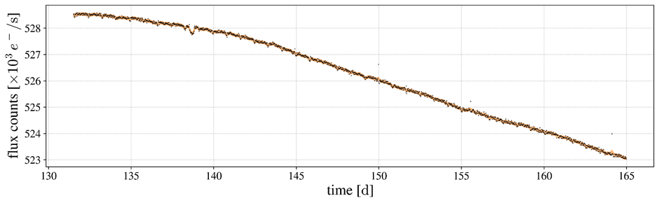
This dataset provides photometric observations from the first science operations phase, suitable for transit detection. Although raw, such a data set is suitable for this study, as further preprocessing measures have been taken. These steps are described in the later segment.

Prior filtering for the detection of Kepler-10b was done in order to evaluate the quality of detections from a known observational basis. Along with Kepler-10b as the target planet, another known planet, Kepler-10c, is also present. All these factors further enhance the quality of this study by providing a richer observation context for better detection potential.

Theoretical Background: BLS Transit Model

The algorithm considers a strict periodic signal with period that alternates between two discrete brightness levels: A higher level, representing the star’s normal brightness (out-of-transit flux), and a lower level, representing the transit (in-transit flux). It assumes that the dip in the light curve looks like a “box” with a quick drop in brightness, then a steady period of low brightness, followed again by a sudden rise to normal.

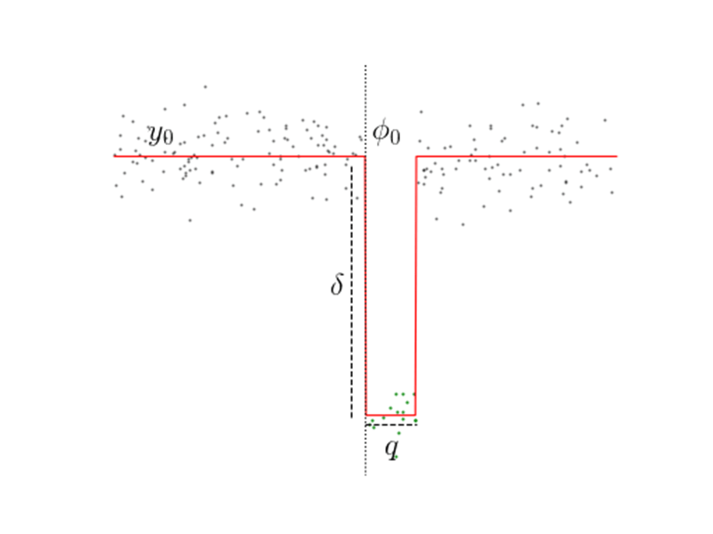
The total period is divided into smaller transit durations represented by a fractional value ranging from 1%-5 %. Now, assuming that the mean of the signal is zero, H can be expressed as:

(1)  

Where H is the out-of-transit level, L is the in-transit level, and q is the fractional transit duration.
This expression helps us derive the transit depth– the difference between H and L:

(2)  

To link the observed transit depth to a physical system, we can also approximate it as the planet-to-star radius ratio:

(3)  

Where, is the radius of the planet, and is the radius of the star.
This inferred transit depth is computed over all the folded light curve segments, where the BLS algorithm recovers the best periods of transiting planets by fitting a box-shaped model into the light curve data.

The transit epoch () is also evaluated alongside this, which is the time corresponding to the first observed mid-transit.
It is used as a reference point to align the folded light curve with the model transit signal.
Hence, the algorithm simultaneously searches over the following parameters:

• P₀, the orbital period,
• q, the fractional transit duration or phase,
• L, in-transit flux,
• H, out-of-transit flux,
• and , epoch of mid-transit.

The inherent property of the BLS method to specifically detect box-shaped signals is what differentiates it from other methods. Using a predetermined shape also gives the algorithm a significant advantage in efficiency over other techniques that detect all types of periodic variation. However, since the algorithm only assumes two levels of the light curve, all other features that are expected to appear in planetary transits are ignored. Hence, the gradual ingress and egress phases, too, are ignored (e.g.,¹³ ). This does not affect calculations significantly as these phases are short compared to the transit. Another effect ignored is the limb-darkening effect, shown to be small in the case of HD 209458¹⁴. This is justified when only concentrating on BLS as a detection tool. For such a case with a slanted ingress and egress (eg, smaller planets), BLS may not be able to accurately infer parameters (transit depth, etc.), but the inaccuracy is borderline and does not significantly affect results.

Preprocessing of the Kepler Data

The preprocessing steps are performed to enhance the detectability of transit signals by reducing outliers, long-term stellar variations, and instrumental noise, which could otherwise obscure transit signals. Additionally, this step is necessary to prevent the detection of false transits. This is done on Google Colab, using Python. Libraries, namely Lightkurve, NumPy, Matplotlib, and  SciPy, are used.

Data Acquisition. The target pixel file for KIC 11904151 (Q1, long cadence) is first downloaded via Lightkurve from the MAST archive. The light curve is then extracted using the default aperture mask provided by the Kepler pipeline. The default aperture mask is a pre-defined set of pixels selected by the pipeline to extract the light curve.

Smoothing. A moving average with Gaussian weights is utilized for smoothing the light curve. Hence, for this process, the original light curve values are reversed and stored in the variable lc_reversed, which is further used for mirror padding via slicing. A window size of  11 is defined; required to define the number of data points from the flux values to be included in the smoothing process, at each iteration.

Another variable, named lc_padded, is defined, which serves as the main padded array. In this context, the “main padded array” is utilized to contain preliminary values when processing, from which data is later extracted to produce the final output of the smoothed light curve. Secondly, it is also used for properly containing assigned data points. It is initially assigned a zero-initialized array, added by the multiplied value of twice the pad size (initialized in an earlier step), ensuring proper memory is allocated for the flux values:

lc_padded = np.zeros(len(lc.flux.value) + 2*pad_size)

This padding process is also necessary to avoid problems relating to edge effects and ensures that all data points are treated equally throughout the algorithm. In the following steps, a mirroring technique is used for padding the margins of the array. The data points from the reversed array (lc_reversed) get assigned to the beginning and end of the padded array (lc_padded). This gives a mirrored structure to the margins of lc_padded. The original light curve was reversed in this manner for the sole purpose of replicating a mirror-like reflection of the data points, and also to simplify the implementation logic. The first and last values corresponding to the window calculation of this array reflect their neighbouring values.

A Gaussian weight function is implemented, centering indices around 0. This allows for higher weightage on the data points near the center and lower weightage on those near the edges. Doing so allows for the implementation to be further accurate and concise by better representing localized trends, as expected in real observations. It uses the formula:

(4)  

This function returns the normalized weights by dividing each weight by the total sum, i.e, weights / (sum)weights, ensuring that the overall sum of the weights equals 1. This measure is taken such that the scaling is correct, avoiding distorted values that can result from uneven scaling.

In the subsequent steps, a variable, smoothed_lc, to store the smoothed light curve’s data points, is initialized with a zero array. The logic for this is:

sigma = 3.0

smoothed_lc = np.zeros(len(lc.flux.value))

for i, _ in enumerate(smoothed_lc):

captured_window = lc_padded[i:i+window]

smoothed_lc[i] = np.dot(captured_window, weights(sigma))

Therefore, a for-loop is iterated over this array.  The moving average is implemented here specifically. The line: captured_window = lc_padded[i:i+window] implements the “moving” aspect of the algorithm, selecting a window of data points at each iteration. Each data point is computed over the same number of times, as discussed earlier. A dot product of the selected values and Gaussian weights is computed and stored in the previously mentioned variable, smoothed_lc. Hence, after all operations are performed, smoothed_lc gives us the final smoothed light curve. Consequently, the overall transit signal becomes clearer as short-term noise is reduced.

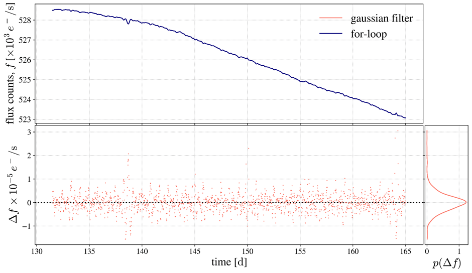
Residual Analysis. As a means of verification, a separate Gaussian filter is applied using SciPy’s gaussian_filter1d function. We generate a graph that compares the manually implemented smoothing method and SciPy’s filter. This serves both as a visualization of the manually processed smoothed light curve and a comparison to an idealized output. Both are smoothed curves plotted against time and labeled accordingly for clarity.

Additionally, a residual plot is also included, illustrating the accuracy of the manual implementation by highlighting fractional differences between the two smoothing methods. This is calculated by applying: 1 − (manual_smoothed / gaussian_smoothed), allowing for visualization of the relative deviation at each point along the light curve.

Normalization. Normalization of the smoothed light curve is now done by dividing by the maximum value of the smooth light curve. This is done to standardize and scale the flux such that the peak becomes 1, and also prepare it for further analysis. This is followed by detrending the new normalized light curve (normalized_lc), which is done using SciPy’s savgol_filter. The computation of this is done by dividing the normalized lc by the resulting trend:

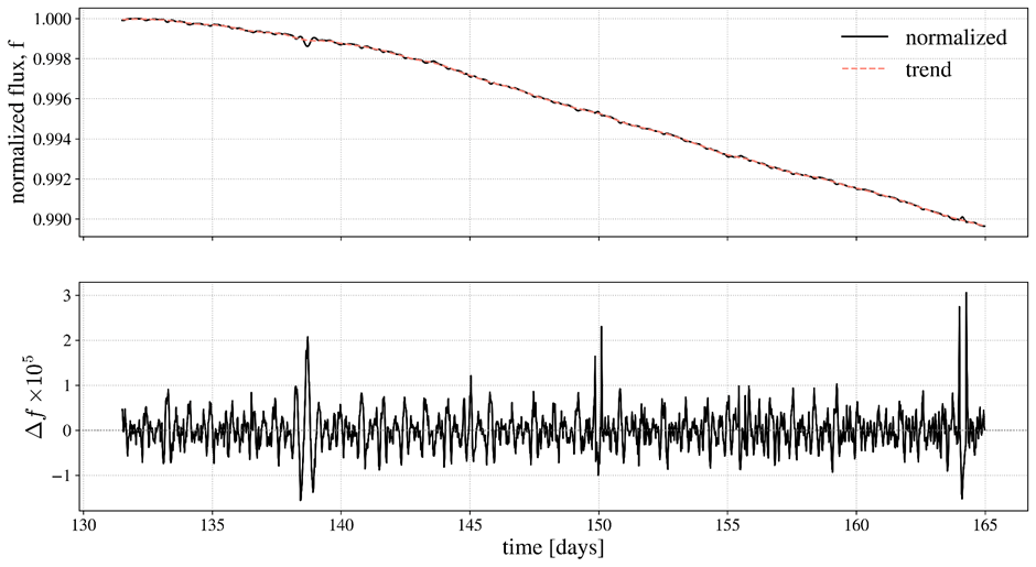
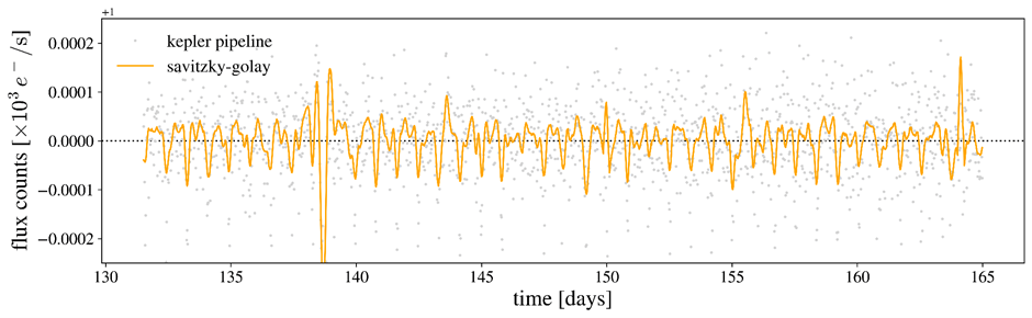
Detrending. Detrending helps us filter the data, removing long-term stellar variation and revealing the overall trend of the light curve. This is useful to isolate short-term features such as transits by identifying subtle dips in the curve, which broader fluctuations would otherwise mask. Hence, a plot is presented for each of these processes, showing the differences between them.

Formulating the BLS Algorithm and Evaluating Uncertainties

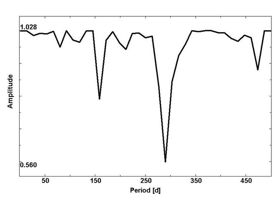
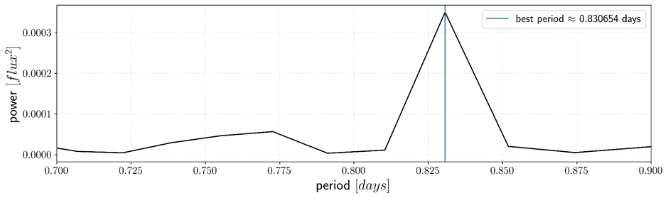
Best-Period Detection. The period, which is essential to modelling the light curve, is calculated with this step. A discrete Fourier Transform (DFT) is computed over the detrended light curve (y), and is stored in fourier. A sampling interval of time[1] – time[0]is then defined to evaluate the frequency. This step allows us to eyeball the values, i.e., aids us in detecting a suitable “best period” to fold our light curve over. In this case, DFT was solely used to detect the most dominant signal as a way of simplifying and efficiently computing the best period detection process. The BLS method is justified in the later steps, whilst being used in model fitting.  Further, the inferred values are masked to retrieve only the non-zero frequencies. The period and power are then calculated using 1 / freq and by squaring the absolute value of fourier, respectively. It is done by:

fourier = fft(y)

sampling_interval = time[1] – time[0]

freq = fftfreq(len(time), d=sampling_interval)

mask = freq > 0

freq = freq[mask]

fourier = fourier[mask]

periods = 1 / freq

power = np.abs(fourier)**2

Each frequency corresponds to a repeating pattern in the light curve. The period calculated gives us the time (in days) it takes for the pattern to repeat. The pattern is of a sinusoidal shape in this case, because DFT models signals using sine and cosine functions, and cannot capture box-shaped dips directly.  BLS is later utilized in searching for such dips. Also, the power at each period gives us the intensity of the signal, i.e, it reflects how strong the signal is. A higher power in certain periods indicates strong periodic signals, which suggest an increased probability in the presence of transits.

The best_period is calculated using:

best_period = periods[np.argmax(power)] Hence, a function np.argmax is used, which returns the index of the maximum value of power. This index is used to retrieve a corresponding value from periods, which in turn gives us the point at which the highest value of power; the strongest periodic signal, is recorded from the frequency domain.

Phase-Folding. The light curve is mapped out here. The box model fits over the phase-folded light curve, and as such, this step lays the groundwork for box-fitting. After retrieving the best period, we infer the epoch, in days. The value is stored in a variable named epoch_time and is calculated by:

 epoch_time = time[np.argmin(y)]

The np.argmin function is used as to find the index of the minimum value from time, roughly corresponding to the center of a transit. It can also be represented as T0 (=epoch), through which the process of phase-folding is performed, using it as reference. This step is merely a formal parameter and serves as an approximation. It is performed solely to fold the data. Further accurate re-centering is performed in later steps.

The data is wrapped in a LightCurve object such that it is easily derivable for further analysis. The data is then phase folded. An extraction process to derive the folded light curve is followed using:

folded = lc_object.fold(period=best_period, epoch_time=epoch_time)

folded_lc = folded.flux.value

phase = folded.time.value

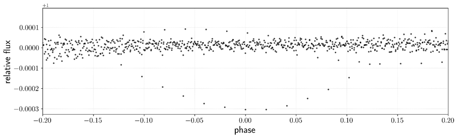
This process maps the time series data onto a single period of the planet’s orbit such that all the repeating signals are stacked on each other, ensuring each transit appears at the same phase. This helps us visualize the data more clearly. Hence, the best period and epoch inferred in the earlier steps are utilized to perform the folding.

Even after folding, the transits stacked up may not align at the epoch, causing a shift in the dips. fold() centers the transits around the epoch symmetrically, but may not necessarily ensure physical accuracy. Therefore, to clarify this, the transits are re-centered manually:

shift = phase[np.argmin(folded_lc)]

phase = phase – shift

By subtracting the shift, i.e., the phase at which the dip occurs, from all the phase values, all the transits are centered at the epoch, simplifying model fitting.

To verify that the phase shifts correctly centers the transit at the epoch, the folded light-curve is sliced into two halves: each corresponding part taken before and after the transit center. The mean fluxes are calculated individually for both these halves (excluding the in-transit dip), and their ratio is calculated. A ratio close to 1 shows that the transit is symmetrically centered and that the baseline is consistent on both sides. Another version of the folded light curve, using binned data values is also tested with this process, but when comparing, it is found out that the unbinned version shows a ratio closer to 1. Binning should have helped reduce noise, but in this case, slightly distorts the transit shape. Hence, since the unbinned values show better symmetry, they were further used for analysis.

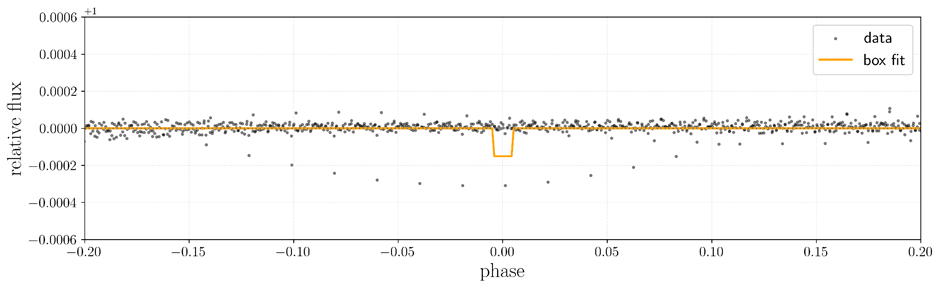
Fitting the Box Model. Values of transit depth (d) and fractional duration (q) are noted for future use from the phase-folded plot. The folded light curve is then normalized; the baseline flux is set to 1, such that the in-transit flux falls below 1 when calculated. This is performed by:

out_of_transit = (np.abs(phase) > 0.05)

baseline = np.median(folded_lc[out_of_transit])

flux = folded_lc / baseline

For example, if the baseline is 0.98, the calculation would follow as: 0.98 – d while fitting the box model, which distorts the fit and renders it meaningless. Hence, this step ensures that the relative transit depth is measured correctly.

A function for the box model is now defined. Inputs for the phase, transit depth, fractional duration, and the center value are taken. These values have already been defined in the previous steps, the exception being center, for which it is initialized with 0, assuming as such for initial visualization. This variable ensures that the box model can shift along the phase axis to match the transit’s center. This flexibility is essential as a rigid box model fixed at a single phase would otherwise fail to accurately match transits that occur at slightly offset positions, resulting in inaccuracy. Though this step does not correct the box-shape mismatch of BLS, it still improves the model’s ability to match real transit signals, albeit marginally. It is given by:

def box_model (phase, d, q, center):

  box_fit = np.ones_like(phase)

  mask = (phase >= center – q/2) & (phase <= center + q/2)

  box_fit[mask] -= d

  return box_fit

Another variable,  box_fit, is initialized with ones to construct the baseline and later input the in-transit flux. A Boolean mask is then created for the same purpose: to detect and input the in-transit flux values into the array. For all phase values that fall within the range defined by q at a specified center, the baseline drops by d, i.e., the transit depth. This replicates a temporary dimming of light based on the given parameters.

Defining Chi-Squared. Using the formula:

(5)  

We define the Chi-Squared statistic used to determine the quality of the approximated box model’s fit, i.e, to estimate how confident we are in the inferred parameters of the box model.
represents the flux values, and the box model over the flux values.
A constant variance is estimated from the out-of-transit scatter, being used to weigh all data points equally.

This is performed by defining a function chi_squared, utilizing the above formula. This returns a single scalar value representing the total deviation of the box fit from the flux. In this case, we assume all errors to hold the same weight (homoscedasticity). This affects the absolute scaling of , yet does not affect the best-fit parameters because their mean remains the same.

Grid Search Function. To find the best-fit parameters characterizing the physical dips in the light curve, a grid search is implemented. This search manually loops over a range of arrays consisting of possible values, and is given by:

def grid_search(q_bounds, d_bounds, center_bounds):

    q_arr = np.linspace(*q_bounds, 50)

    d_arr = np.linspace(*d_bounds, 50)

    center_arr = np.linspace(*center_bounds, 50)

    chi2_arr = np.ones(shape=(len(q_arr), len(d_arr), len(center_arr)))

    for i, q in enumerate(tqdm(q_arr)):

        for j, d in enumerate(d_arr):

          for k, center in enumerate(center_arr):

            box_fit = box_model(phase, d, q, center)

            chi2 = chi_squared(y_obs=flux, y_exp=box_fit)

            chi2_arr[i, j, k] = chi2

    argmin = chi2_arr.argmin()

    i_best, j_best, k_best = np.unravel_index(argmin, chi2_arr.shape)

    return q_arr[i_best], d_arr[j_best],  center_arr[k_best]

Inputs for the transit depth boundary, fractional duration boundary, and center boundaries are taken. For each possible combination of these inputs, a model light curve is generated using the box_model function, and a comparison is drawn to the observed light curve using chi_squared. The output is then stored in the variable chi2_arr. Once done computing for the best-fit values, the index of the minimum chi-squared value is identified. This is implemented to find the fit with the least residuals. Such a fit would give the most accurate model from amongst the specified ranges. By using np.unravel_index, these values are extracted and stored. Though this method is computationally intensive, under the assumption that the optimization is convex, it should identify the global minimum and be meaningful under these conditions.

Evaluating Uncertainties. The optimal fractional duration, transit depth, and center are then determined over specified ranges and stored. Before evaluating uncertainties though, the phase is shifted according to the best-fit center value to align the transit at the epoch. Another box model is then constructed, which utilizes all the best found parameters. This step is performed to ensure fitting against a clearly centered signal. Without this, the uncertainty measurement would be distorted due to misalignment. It is given by:

phase_shifted = phase – center_best

best_fit = box_model(phase_shifted, d_best, q_best, center=0)

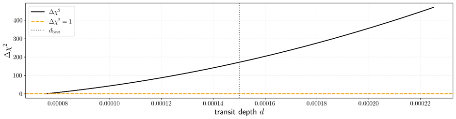
Since the uncertainty of the planet-to-star ratio is evaluated here, the transit depth’s uncertainty is what concerns the analysis the most. Therefore, for this, an uncertainty estimation is performed using a chi-squared profile. It is to find the mismatch between the observed data and the model, giving us an amount by which d is allowed to differ.

d_best = d_best

d_values = np.linspace(0.5 * d_best, 1.5 * d_best, 500)

chi2_vals = []

for d in d_values:

model = box_model(phase_shifted, d=d, q=q_best, center=0)

chi2 = chi_squared(y_obs=flux, y_exp=model)

chi2_vals.append(chi2)

chi2_vals = np.array(chi2_vals)

chi2_min = np.min(chi2_vals)

threshold = chi2_min + 1  # 1-sigma for 1 parameter

Multiple points of d are calculated, through which the uncertainty is tested. For every value, a model is computed whose uncertainty is calculated through chi-squared consequently. The minimum of these values is then found, over which a 1-sigma confidence interval is calculated. This threshold is used because we are considering only one parameter, and do not want to exceed the minimum by more than 1.

Next, a Boolean array for values where the chi-squared is within the 1-sigma range is generated; further used as a mask to obtain the statistically good fits. These values are separated into two halves, both of which are used to find the range within which the uncertainty is acceptable. Code to accompany:

mask = chi2_vals <= threshold

left = d_values[(d_values < d_best) & mask]

right = d_values[(d_values > d_best) & mask]

if len(left) > 0 and len(right) > 0:

    d_lower = left[-1]

    d_upper = right[0]

    sigma_d = 0.5 * (d_upper – d_lower)

    print(f”sigma_d = {sigma_d:.8f}”)

As a result, the two limits are computed by using if. The left-most value in the range is picked as the lower bound, and the right-most value is picked as the upper bound. Half of this total width of the interval is the 1-sigma uncertainty, as the uncertainty calculated is centered around d_best, assuming the distribution is roughly symmetric. Therefore, the uncertainty in transit depth is printed: calculating how sensitive the result is to changes in the transit depth.

The radius of the planet to star ratio is consequently computed, inferring it from the square root of d_best. This can be understood by the following formula:

(6)  

Finally, the uncertainty is derived using a standard uncertainty propagation to convert the error in depth into an error in the radius ratio, giving us the radius ratio error.

Results

A periodic transit-like signal was identified via manual methods of pre-processing and phase folding. A box-fitting model function was implemented via a weighted chi-squared function to a flux-normalized Kepler light curve- KIC 11904151 from the Q1 phase. The best-fit period, which was computed with a discrete Fast Fourier Transform and inferred through phase-folding and inspection, was estimated at 0.830654 days. The parameters input into the grid search were:

• Fractional duration (q_bounds) = 0.01 to 0.1
• Transit depth (d_bounds) = 0.00015 to 0.00025
• Center / Mid transit phase (c_bounds) = -0.02 to 0.02

With results obtained through grid search minimization by chi-squared statistics:

• Fractional duration (q_best)  = 0.01
• Transit depth (d_best) = 0.00015
• Mid transit phase (c_best) = 0.019

Using a standard approximation, the planet-to-star radius ratio is estimated as:

(7)  

Uncertainty in depth was calculated via chi-squared profiling, yielding a minimum chi-squared statistic of .
However, the resulting chi-squared statistic showed some degeneracy, even though the best-fit parameters were well within the grid and showed reasonable agreement with values in the updated NASA Exoplanet archive (depth 191.9 ppm).
It aligns more closely with Batalha’s published values. The chi-squared curve is slowly rising away from the minimum, indicating partial degeneracy, implying that the transit depth is weakly constrained.

Hence, the final result is given as:

(8)  

When comparing the implemented model with the NASA-published value for Kepler 10b ( 0.01233), a close agreement is observed, with a difference of less than 1%. The inferred transit depth of 150 ppm also aligns well with the reported depth of 152 4 ppm¹⁵. Though it is important to note that the uncertainty reported in this paper does not incorporate formalities such as systematic noise, finite sampling, or photometric errors (limb darkening). Therefore, it underestimates the true uncertainty. Nonetheless, the resemblance in transit depth and radius ratio accounts for the robustness of the detection and modeling methodology.

The final parameters and derived quantities are summarized in Table 1.

Parameter	Symbol	Value
Orbital Period (in days)	P0	0.830654
Fractional transit duration	q	0.01
Transit depth	d	0.00015 (150 ppm)
Mid transit phase	—	0.019
Minimum χ²		1835.769
Planet-star radius ratio		0.01225  0.00002

Discussion

The BLS algorithm implemented in this paper was found to be particularly suitable in detecting transit-like signals consisting of parameters resembling Kepler 10b, suggesting that the implemented detection method is capable of detecting with sensitivity and precision. The detected planet-to-star ratio very closely resembles NASA’s published values and is within 1% proximity. Hence, this reflects the robustness of the preprocessing as well as the fitting pipeline. Even with a simplified and manual implementation, BLS can successfully and accurately recover meaningful transit parameters. The objective of this paper was to be able to characterize how well the BLS method infers physical characteristics, which is met with promising correspondence. However, the chi-squared profiling exhibited a shallow rise, indicating degeneracy in the transit depth. This implies that while the best-fit values are plausible, the uncertainty is underestimated, as inferred from Batalha et al. (2011). This is most likely caused due to ignoring systematic errors– instrumental noise, stellar variability, etc., and the absence of limb-darkening that constrains the confidence in precision estimates. Still, after drawing a comparison with NASA’s published values, the credibility of the method is reinforced.

Findings imply that even a manually implemented BLS algorithm is capable of producing robust results. This validates the core strength of the algorithm and highlights its accuracy. The model used is also very simple– it does not consider assumptions owing to limb darkening and noise modelling. Hence, this justifies that even simple models can accurately produce results, as proved above. It also goes on to show that accurate exoplanet detection is possible without complex tools. Hence, this study also successfully shows that exoplanet detection is not limited to high-end pipelines and challenges the assumption that such pipelines are necessary. It also fills a significant educational gap by demonstrating that exoplanet detection is possible with minimal infrastructure. It bridges the gaps between advanced astrophysical research and an accessible workflow. Reproduction of this implementation can also be done fairly easily, which makes it accessible to students and educators with minimal resources. The ability to detect meaningful signals using fundamental tools also offers a baseline for more sophisticated future work. Added model complexity can be evaluated against an already validated implementation. This study, henceforth, makes exoplanet detection more replicable with minimum complexity.

Multiple simplifications and assumptions were made to make the study reproducible and easily comprehensible. Astrophysical effects such as limb darkening, ingress/egress curvature were not taken into consideration. This is justified because, while our study includes parameter estimation,  BLS is used primarily as a detection statistic, in its first principles. While limb darkening introduces biases in the ratio¹⁶, it has not been utilized due to the practical limitations of the study. Another assumption made was that the transit shape was interpreted as a flat-bottomed box, as opposed to physical transits. This may misrepresent real photometric features, but it does not undermine key characteristics like transit depth.

When computing the uncertainty, many problems had arisen due to simplifying assumptions. We assume a constant variance estimated from the out-of-transit flux and that the χ² surface is locally convex. This can also explain the inaccuracy of the inferred uncertainty statistic, and relates to the degeneracy caused while showcasing precision estimation. Effects not explicitly accounted for, such as stellar variability, etc., have caused significant underestimation of the uncertainty.

DFT was used as a means to identify the best period; this approach varies with different signals. Kepler 10b’s period was easily detected due to its high clarity in its signal, but this approach is not optimal for more ambiguous cases with weaker, noisier signals.

References

1. S. Seager. On the unique solution of planet and star parameters from an extrasolar planet transit light curve. The Astrophysical Journal. Vol. 585, pg. 1038–1055, 2002. https://doi.org/10.1086/346105. [↩] [↩] [↩] [↩]
2. J. W. Cooley and J. W. Tukey. An algorithm for the machine calculation of complex Fourier series. Mathematics of Computation. Vol. 19, pg. 297–301, 1965. https://doi.org/10.1090/S0025-5718-1965-0178586-1. [↩]
3. J. H. Steffen, D. C. Fabrycky, E. B. Ford, J. A. Carter, J.-M. Désert, F. Fressin, M. J. Holman, J. J. Lissauer, A. V. Moorhead, J. F. Rowe, G. Torres, and W. F. Welsh. Transit timing observations from Kepler: III. Confirmation of four multiple-planet systems by a Fourier-domain study of anti-correlated transit timing variations. The Astrophysical Journal. Vol. 756, pg. 186, 2012. https://doi.org/10.1088/0004-637X/756/2/186. [↩]
4. R. F. Stellingwerf. Period determination using phase dispersion minimization. The Astrophysical Journal. Vol. 224, pg. 953–960, 1978. https://doi.org/10.1086/156444. [↩]
5. A. Schwarzenberg-Czerny. Fast and statistically optimal period search in uneven sampled observations. The Astrophysical Journal Letters. Vol. 460, pg. L107–L110, 1996. https://doi.org/10.1086/309985 [↩]
6. G. Kovács, S. Zucker, and T. Mazeh. A box-fitting algorithm in the search for periodic transits. Astronomy & Astrophysics. Vol. 391, pg. 369–377, 2002. https://doi.org/10.1051/0004-6361:20020802. [↩] [↩] [↩] [↩] [↩]
7. A. Collier Cameron, D. M. Wilson, R. G. West, L. Hebb, X. Wang, S. Aigrain, F. Bouchy, D. J. Christian, W. I. Clarkson, B. Enoch, C. A. Haswell, C. Hellier, K. Horne, S. R. Kane, T. A. Lister, B. Loeillet, P. F. L. Maxted, M. Mayor, I. McDonald, C. Moutou, A. J. Norton, N. Parley, F. Pont, D. Pollacco, R. Ryans, I. Skillen, R. A. Street, S. Udry, and P. J. Wheatley. Efficient identification of exoplanetary transit candidates from SuperWASP light curves. Monthly Notices of the Royal Astronomical Society. Vol. 380, pg. 1230–1244, 2007. https://doi.org/10.1111/j.1365-2966.2007.12195.x. [↩]
8. S. R. Jacklin, M. B. Lund, J. Pepper, and K. G. Stassun. Transiting planets with LSST. II. Period detection of planets orbiting 1 M⊙ hosts. The Astronomical Journal. Vol. 150, pg. 34, 2015. https://doi.org/10.1088/0004-6256/150/1/34. [↩]
9. H. Rauer, C. Catala, C. Aerts, T. Appourchaux, W. Benz, A. Brandeker, J. Christensen-Dalsgaard, M. Deleuil, L. Gizon, M.-J. Goupil, M. Güdel, E. Janot-Pacheco, M. Mas-Hesse, I. Pagano, G. Piotto, D. Pollacco, Ċ. Santos, A. Smith, J.-C. Suárez, R. Szabó, S. Udry, V. Adibekyan, Y. Alibert, J.-M. Almenara, P. Amaro-Seoane, M. Ammler-von Eiff, M. Asplund, E. Antonello, S. Barnes, F. Baudin, K. Belkacem, M. Bergemann, G. Bihain, A. C. Birch, X. Bonfils, I. Boisse, A. S. Bonomo, F. Borsa, I. M. Brandão, E. Brocato, S. Brun, M. Burleigh, R. Burston, J. Cabrera, S. Cassisi, W. Chaplin, S. Charpinet, C. Chiappini, R. P. Church, Sz. Csizmadia, M. Cunha, M. Damasso, M. B. Davies, H. J. Deeg, R. F. Díaz, S. Dreizler, C. Dreyer, P. Eggenberger, D. Ehrenreich, P. Eigmüller, A. Erikson, R. Farmer, S. Feltzing, F. de Oliveira Fialho, P. Figueira, T. Forveille, M. Fridlund, R. A. García, P. Giommi, G. Giuffrida, M. Godolt, J. Gomes da Silva, T. Granzer, J. L. Grenfell, A. Grotsch-Noels, E. Günther, C. A. Haswell, A. P. Hatzes, G. Hébrard, S. Hekker, R. Helled, K. Heng, J. M. Jenkins, A. Johansen, M. L. Khodachenko, K. G. Kislyakova, W. Kley, U. Kolb, N. Krivova, F. Kupka, H. Lammer, A. F. Lanza, Y. Lebreton, D. Magrin, P. Marcos-Arenal, P. M. Marrese, J. P. Marques, J. Martins, S. Mathis, S. Mathur, S. Messina, A. Miglio, J. Montalban, M. Montalto, M. J. P. F. G. Monteiro, H. Moradi, E. Moravveji, C. Mordasini, T. Morel, A. Mortier, V. Nascimbeni, R. P. Nelson, M. B. Nielsen, L. Noack, A. J. Norton, A. Ofir, M. Oshagh, R.-M. Ouazzani, P. Pápics, V. C. Parro, P. Petit, B. Plez, E. Poretti, A. Quirrenbach, R. Ragazzoni, G. Raimondo, M. Rainer, D. R. Reese, R. Redmer, S. Reffert, B. Rojas-Ayala, I. W. Roxburgh, S. Salmon, A. Santerne, J. Schneider, J. Schou, S. Schuh, H. Schunker, A. Silva-Valio, R. Silvotti, I. Skillen, I. Snellen, F. Sohl, S. G. Sousa, A. Sozzetti, D. Stello, K. G. Strassmeier, M. Švanda, Gy. M. Szabó, A. Tkachenko, D. Valencia, V. Van Grootel, S. D. Vauclair, P. Ventura, F. W. Wagner, N. A. Walton, J. Weingrill, S. C. Werner, P. J. Wheatley & K. Zwintz. The PLATO 2.0 mission. Experimental Astronomy. Vol. 38, pg. 249–330, 2014. https://doi.org/10.1007/s10686-014-9383-4. [↩]
10. W. Benz, C. Broeg, A. Fortier, N. Rando, T. Beck, M. Beck, D. Queloz, D. Ehrenreich, P. F. L. Maxted, K. G. Isaak, N. Billot, Y. Alibert, R. Alonso, C. António, J. Asquier, T. Bandy, T. Bárczy, D. Barrado, S. C. C. Barros, W. Baumjohann, A. Bekkelien, M. Bergomi, F. Biondi, X. Bonfils, L. Borsato, A. Brandeker, M.-D. Busch, J. Cabrera, V. Cessa, S. Charnoz, B. Chazelas, A. Collier Cameron, C. Corral Van Damme, D. Cortes, M. B. Davies, M. Deleuil, A. Deline, L. Delrez, O. Demangeon, B. O. Demory, A. Erikson, J. Farinato, L. Fossati, M. Fridlund, D. Futyan, D. Gandolfi, A. Garcia Munoz, M. Gillon, P. Guterman, A. Gutierrez, J. Hasiba, K. Heng, E. Hernandez, S. Hoyer, L. L. Kiss, Z. Kovacs, T. Kuntzer, J. Laskar, A. Lecavelier des Etangs, M. Lendl, A. López, I. Lora, C. Lovis, T. Lüftinger, D. Magrin, L. Malvasio, L. Marafatto, H. Michaelis, D. de Miguel, D. Modrego, M. Munari, V. Nascimbeni, G. Olofsson, H. Ottacher, R. Ottensamer, I. Pagano, R. Palacios, E. Pallé, G. Peter, D. Piazza, G. Piotto, A. Pizarro, D. Pollaco, R. Ragazzoni, F. Ratti, H. Rauer, I. Ribas, M. Rieder, R. Rohlfs, F. Safa, M. Salatti, N. C. Santos, G. Scandariato, D. Ségransan, A. E. Simon, A. M. S. Smith, M. Sordet, S. G. Sousa, M. Steller, G. M. Szabó, J. Szoke, N. Thomas, M. Tschentscher, S. Udry, V. Van Grootel, V. Viotto, I. Walter, N. A. Walton, F. Wildi & D. Wolter. The CHEOPS mission. Experimental Astronomy. Vol. 51, pg. 109–151, 2021. https://doi.org/10.1007/s10686-020-09679-4. [↩]
11. J. N. Winn. Transits and occultations. In Exoplanets. 2010. https://doi.org/10.1007/978-3-540-74008-7_14. [↩]
12. T. N. Gautier, N. M. Batalha, W. J. Borucki, W. D. Cochran, E. W. Dunham, S. B. Howell, J. M. Jenkins, D. W. Latham, J. J. Lissauer, J. F. Rowe, D. D. Sasselov, S. Seager, G. Torres, and L. M. Walkowicz. The Kepler follow-up observation program. arXiv e-prints, 2010. https://doi.org/10.48550/arXiv.1001.0352. [↩]
13. P. D. Sackett, M. D. Albrow, J.-P. Beaulieu, J. A. R. Caldwell, C. Coutures, M. Dominik, J. Greenhill, K. Hill, K. Horne, U.-G. Jørgensen, S. Kane, D. Kubas, R. Martin, J. W. Menzies, K. R. Pollard, K. C. Sahu, J. Wambsganss, R. Watson, and A. Williams. PLANET II: a microlensing and transit search for extrasolar planets. In Bioastronomy 2002: Life Among the Stars, edited by R. Norris and F. Stootman, IAU Symposium, Vol. 213, pg. 35, 2004. https://ui.adsabs.harvard.edu/abs/2004IAUS..213…35S [↩]
14. H. J. Deeg, R. Garrido, and A. Claret. Probing the stellar surface of HD 209458 from multicolor transit observations. New Astronomy. Vol. 6, pg. 51–60, 2001. https://doi.org/10.1016/S1384-1076(01)00044-6. [↩]
15. N. M. Batalha, W. J. Borucki, S. T. Bryson, L. A. Buchhave, D. A. Caldwell, J. Christensen-Dalsgaard, D. Ciardi, E. W. Dunham, F. Fressin, T. N. Gautier, R. L. Gilliland, M. R. Haas, S. B. Howell, J. M. Jenkins, H. Kjeldsen, D. G. Koch, D. W. Latham, J. J. Lissauer, G. W. Marcy, J. F. Rowe, D. D. Sasselov, S. Seager, J. H. Steffen, G. Torres, G. S. Basri, T. M. Brown, D. Charbonneau, J. Christiansen, B. Clarke, W. D. Cochran, A. Dupree, D. C. Fabrycky, D. Fischer, E. B. Ford, J. Fortney, F. R. Girouard, M. J. Holman, J. Johnson, H. Isaacson, T. C. Klaus, P. Machalek, A. V. Moorhead, R. C. Morehead, D. Ragozzine, P. Tenenbaum, J. Twicken, S. Quinn, J. VanCleve, L. M. Walkowicz, W. F. Welsh, E. Devore, and A. Gould. Kepler’s first rocky planet: Kepler-10b. The Astrophysical Journal. Vol. 729, pg. 27, 2011. https://doi.org/10.1088/0004-637X/729/1/27 [↩]
16. N. Espinoza and A. Jordán. Limb darkening and exoplanets: testing stellar model atmospheres and identifying biases in transit parameters. Monthly Notices of the Royal Astronomical Society. Vol. 450, pg. 1879–1899, 2015. https://doi.org/10.1093/mnras/stv744 [↩]