
Abstract
With the legalization of sports betting in the United States in 2018, a new academic context for studying risk preference opened up beyond traditional retail trading and gambling. However, research that directly tests the association between stock market fluctuations and changes in sports betting behavior remained sparse. This paper aimed to address such a gap by examining whether movement in the stock market was linked to a shift in sports betting volume, specifically by quantifying the relationship between monthly stock market performance and sports betting handle. Based on Prospect Theory, I hypothesized that because individuals in the loss domain become more risk seeking, stock market downturn would be correlated with an increase in betting market volume. Employing a multi-step empirical methodology that included time-series visuals, Pearson correlation analysis, Elastic Net regression, and generalized least squares regression with autoregressive error (GLSAR), I analyzed monthly sports betting handle of six states against major stock index values, bettable sporting event exposure variables, and state macroeconomic indicators. My results showed a statistically significant negative relationship between movements in the S&P 500 and sports betting handle in New York State, albeit in a state-specific manner. These results suggested that behavioral theories of risk-seeking in the loss domain may be applicable to the context of sports gambling and offer some possible implications for gambling policy during periods of financial stress.
Keywords: Sports Betting, Risk Preference, Loss Domain, Stock Market, Prospect Theory
Introduction
The recent legalization of US sports betting in 2018 has opened up a new academic context apart from traditional retail trading for the study of risky choice. Since then, online sportsbooks operated by companies including DraftKings and Fanduel have risen dramatically as legal sports betting has become much more accessible. While betting on sports may be considered more recreational and lower stakes than stock trading, the two are both risk-based financial activities that can help build an understanding of behavior under uncertainty.
Besides the fact that not much research has been conducted specifically on sports betting due to how new it is as an industry, existing research still presents many gaps to be filled. For example, gambling in general is often treated as separate from regular stock trading due to its disposable nature1. In addition, most research that looks into sports betting and its legalization either draws similarities between the two, or focuses on sports betting’s effect on trading1,2,3. However, my goal is to examine the effect of stock market performance and trading behavior on sports betting.
While not in the context of sports betting, behavioral economists have studied risk preferences for a long time. In Prospect Theory, Kahneman and Tversky4 make the distinction between two different behavioral responses to loss: loss aversion and risk seeking in the loss domain. The former refers to the idea that at and around the reference point, losses have a larger emotional impact than equivalent gains, causing individuals to try to avoid additional risks for fear of further losses. However, once a person has already experienced a loss that puts them below their reference point, they will begin to exhibit increased risk seeking behavior. This is shown by the convexity of the value function in the loss domain, in which individuals derive more utility from returning to the reference point via a gain than they lose from an equivalent loss. Applied to betting behavior and stock market performance, Prospect Theory predicts that the desire to break even when in the loss domain makes risky behaviors more attractive, suggesting that market downturns may trigger increases in sports betting.
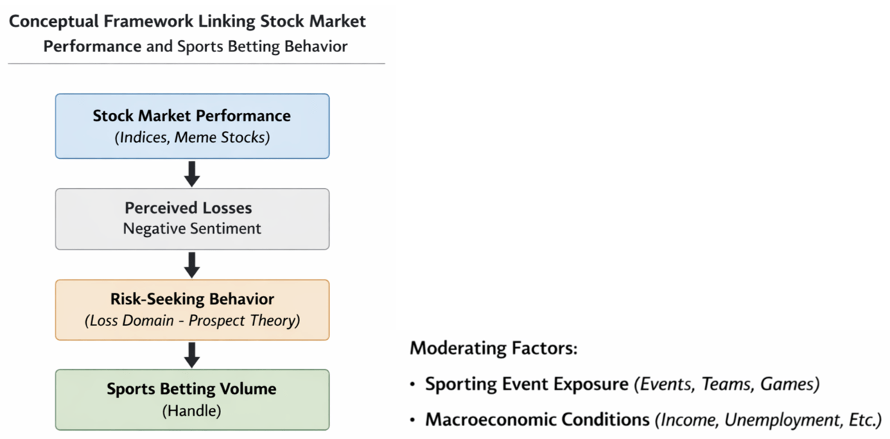
Building off of this theoretical foundation, my study adopts a conceptual framework in which stock market performance is a proxy for changes in the perceived financial state of consumers. I assume that negative stock market movements shift individuals below their reference point, altering risk perception by increasing perceived losses. According to Prospect Theory, this entry into the loss domain will induce greater risk seeking behavior, which is operationalized as an increase in sports betting handle. State exposure to sporting events and broader macroeconomic conditions such as unemployment rate or annual income serve as moderators by shaping the availability of betting opportunities and the economic capacity of individuals.
The idea that confidence may drive people to make irrational decisions has also been very prevalent, whether they are deciding to enter new markets5 like sports betting or believe that success is inevitable. Kahneman and Tversky6 cited this Gambler’s Fallacy, which is the tendency for people to think that a string of losses makes a win more likely when the events are actually independent, as part of their representativeness heuristic. This paper presents a hypothesis that generally aligns with Kahneman and Tversky4 provided that when the stock market goes down, sports betting may increase as people seek to regain what they have lost through a different medium.
Using a variety of econometric methods including Pearson correlation, Elastic Net regression and generalized least squares regression with autoregressive error (GLSAR), my study examines the impact of stock market performance on sports betting handle in several selected states. Predictors include major indices like the S&P 500, which is used as both an indicator of overall stock market performance and portfolio performance of long-term investors, variables for sporting events, and macroeconomic indicators such as state income and unemployment.
The main objective of this paper is to determine whether there is a relationship between stock market performance and sports betting volume, particularly if stock market downturns are associated with increases in sports betting. Through my research, I use empirical quantitative analysis to build on existing theoretical frameworks of risk behavior after loss. This paper extends such theories into the new context of legal sports betting while also carrying implications for policies that can mitigate self-destructive gambling behavior during times of economic downturn. Although legal sports betting presents opportunities for study, it also brings about new risks relating to addiction.
The scope of this study covers six selected US states in which sports betting has been legal for a substantial amount of time, focusing on month-level aggregate data instead of more specific daily trends. However, the recency of sports betting legalization constrains the dataset to only about six or seven years, making it difficult to make long-term conclusions. Nevertheless, my study provides early insight into an emerging sports betting industry.
Literature Review
In this section, I synthesize foundational behavioral theories and existing research on the topic to establish the conceptual framework of my study on the relationship between sports betting and stock market movements. Drawing on behavioral economics and decision theory, I explore two competing predictions about risk taking behavior after financial loss. The literature in this section is organized to show how foundational theories first evolved and where gaps remain, which gives way to the hypothesis that sports betting and stocks move with a negative correlation. While these early frameworks are important for my understanding of risk preference, most focused only on controlled experiments or abstract lotteries rather than real-world behaviors.
Competing Theoretical Views on Risk After Loss
Expected Utility Theory (EUT) and Prospect Theory are two prominent frameworks that provide competing predictions for how the risk taking capacity of individuals will respond to financial losses, such as stock market downturns.
EUT, a cornerstone of traditional economic theory that was first formalized by von Neumann and Morgenstern7, predicts that individuals are risk averse in general and especially so after a reduction in total wealth. The concavity of the standard utility function, which implies diminishing marginal utility of wealth, suggests that a downturn in the stock market would likely deter participation in high risk activities such as sports betting. However, EUT has been criticized over the years due to its unrealistic predictions with large wealth values. For example, Rabin and Thaler8 illustrated that under EUT, any small level of risk aversion over small stakes implies an absurdly high level of risk aversion over large stakes, which revealed an important limitation of EUT: its struggle to explain how people respond to significant financial shocks.
Prospect Theory, introduced by Kahneman and Tversky4 in 1979, diverges from EUT by framing decisions in terms of gains and losses relative to a reference point instead of absolute states of wealth. The central insights of Prospect Theory are loss aversion—that losses have a larger psychological impact than equivalent gains—and that individuals exhibit risk seeking behavior when in the loss domain, suggesting that people may be more willing to engage in speculative betting to recover losses after stock market declines. This theoretical division sparks ambiguity regarding risk preference in the loss domain, as financial losses may either dampen or stimulate gambling activity depending on which theory applies to this situation; my study aims to assess the merit of these two theories when it comes to risk behavior after losses or gains across financial domains.
Refinements and Extensions in Behavioral Economic Theory
Later research has elaborated upon the dynamics of risk preference after loss and recognized other factors such as mental accounting, realization of losses, and perceived control which all play a role in shaping individual responses to loss.
Thaler and Johnson9 introduced two effects that have a strong influence on risk preference: the house money effect suggests that recent gains cause individuals to be more inclined to risk, and the break even effect states that recent losses motivate risk seeking behavior to recover losses. These concepts extend Prospect Theory to view the psychological categorization of outcomes as another key determining factor on risky choice. When applied to the present study, Thaler and Johnson’s research suggests that individuals may increase sports betting either way.
Imas10 provides a more nuanced refinement by making the distinction between realized versus paper losses, concluding that individuals become risk seeking after experiencing unrealized, or paper, losses and risk averse when the losses are realized. This offers a possible explanation for heterogeneity in behavior after market downturn, as some investors may have realized their losses by selling their stock while others may have not. However, as with Thaler and Johnson, such findings emerge from experimental environments and these effects have not been validated in large-scale financial environments, making it unclear whether these behavioral tendencies persist when applied to mobile sports betting platforms.
Cognitive and Emotional Biases in Risk Preference
Other recent behavioral models have emphasized the role of emotion and cognition in shaping risk behavior, deepening the predictions of Prospect Theory by showing that reactions are highly dependent on context and mediated by psychology. This new layer of behavioral insight further complicates the predicted relationship between financial setbacks and speculative activities.
Theories on overconfidence can offer additional insight on risky choices following losses and gains. Moore and Healy11 draw the connection between the difficulty of a task and the perceived skill of an individual, finding that individuals overestimate their abilities when they feel like they have more control. In the context of sports betting, this suggests that people may believe that they have greater ability in predicting sporting event outcomes than macroeconomic movements, which encourages sports betting as an alternative when the stock market experiences a downturn. Their findings build on earlier research by Camerer and Lovallo5, who showed that competitive situations in which outcomes depend on the actions of others make individuals especially prone to overconfidence. This framework applies to speculative domains like sports betting and retail trading, where people overestimate their advantage over the competition.
Affect-based decision theories also emphasize the role that emotional reactions to prior losses play in shaping risk preferences in the future. Loewenstein12 argues that experiences that provoke negative emotions such as market crashes can increase risk aversion due to anticipation of further losses. Similarly, Hertwig13 shows that recalling past losses can reduce tolerance for risk by distorting estimates of probability and overweight unlikely negative outcomes. Loewenstein14 also extends this emotional framework by revealing that utility can also be derived from anticipation of outcomes, meaning that expected disappointment triggered by memories of previous losses may suppress risk seeking behavior, leading to decreased betting activity during bear markets.
However, these mechanisms may also work in the opposite direction and cause risk seeking—if individuals suppress negative feedback, they may discount losses and continue to engage in risky speculative activities. For example, Eil and Rao15 find that individuals selectively discard bad news to maintain their self-esteem, which may foster irrational optimism.
Together, these findings reveal an unresolved tension: whether the emotional impact of losses increases cautious risk averse or overconfident risk seeking behavior. Moreover, most of these studies have been conducted in experimental environments or with data that is self-reported, leaving questions about whether these mechanisms manifest in real-world financial environments such as sports betting or investment.
Mental accounting presents an alternative that further complicates the situation, stating that decisions in different financial domains may be decoupled. For example, individuals may have separate mental budgets for sports betting and investing, meaning that a loss in one domain does not directly translate into risk aversion or seeking in another. This separation may neutralize the effect of stock market movements on betting volume.
While these psychological mechanisms offer rich insights into behavioral theory, such studies rely on controlled environments and do not capture financial behaviors across domains. This presents an empirical gap, especially in the context of recently legalized sports betting, where we may test the effect of stock market movements on sports betting behavior and gain new insight on whether such factors influence cross-domain risk substitution or amplification.
Recent Empirical Advances Bridging Sports Betting and Financial Markets
The past few years have seen a new wave of empirical studies that make the connection between sports betting behaviors and activity in financial markets, filling gaps identified in earlier more theoretical sections. These new studies employ various methods such as natural experiments, panel regressions, sentiment analysis, and event studies to refine classical behavioral theories. In doing this, they reveal that the domains of gambling and investing are more interconnected than previously thought, with sports betting behavior spilling into investor decisions and vice versa.
Impact of Betting on Investor Choices
A major question has been whether gambling acts as a substitute for risky investing or whether it complements it. Using a staggered difference-in-differences model around US legalizations of sports betting by state, Douidar et al.2 finds evidence for the complementarity of gambling with investing. Following the legalization of sports betting, they found that local retail investors increase their preference for speculative “lottery” stocks and exhibit a higher home bias in such local stocks, which suggests that the availability of sports betting increases investor appetite for stock risks instead of displacing it. Their findings complement earlier work by Arthur et al.1 that noted parallels between novel financial instruments and gambling products, suggesting that gamblers may be more inclined to participating in speculative trading. Taken together, recent empirical studies indicate that the introduction of legalized sports betting can amplify risky investment behavior, filling a gap about how new forms of gambling alter investor choices.
Mixed Outcomes in Household Finance
Other studies have examined the impact of sports betting on household financial situations. Baker et al.16 utilize online sportsbooks to quantify impacts on personal finances, finding that increased access to betting does not displace other forms of consumption, but rather crowd out savings and investment particularly for financially constrained families. Within a year of sports betting legalization, they observed significant decreases in brokerage account contributions as well as increases in credit card debt and overdraft fees, echoing concerns about household financial stability. On the other hand, Bersak et al.17 offer a more nuanced perspective using a panel difference-in-difference approach to the Household Pulse Survey, which revealed no significant change in self-reported financial distress or mental health, suggesting that moderate bettors may be capable of absorbing losses from betting without facing immediate hardship. Combined with Baker et al.’s research, these findings show that consequences of sports betting are not evenly distributed, with vulnerable groups experiencing most of the harm. This emerging evidence advances our understanding by zooming in on where financial risks truly lie, challenging the assumption in the previous section “Refinements and Extensions in Behavioral Economic Theory” that new betting opportunities would simply replace other forms of financial risk.
Convergence of Gambling and Trading Behaviors
Early survey evidence by Cox et al.18 estimated that around 4.4 percent of retail investors met the clinical criteria for compulsive gambling, with an additional 3.6 percent demonstrating problem gambling urges. Notably, nearly half of the investors in the study admitted to trading primarily for fun, revealing that a respectable share of stock market activity is motivated by thrill seeking similar to that of a lottery. To build on this, Coloma-Carmona et al.19 employ a latent class analysis on a Spanish dataset, uncovering a “gambling-trader” cohort consisting of around 15 percent of retail investors that is heavily involved in both trading and gambling at high frequencies. In the meantime, a systematic review conducted by Lee et al.20 confirms a strong association between frequent trading and gambling problems, with higher trading frequency or trading assets that are more volatile correlates with more severe gambling disorder symptoms. Additionally, Han and Kumar21 found that stocks that are often traded by speculative retail investors attracted individuals with a high gambling propensity, despite the stocks themselves being overpriced and generating negative abnormal returns. Their findings even further validate the tendency of speculative trading to reflect gambling-like preferences, reinforcing the connection between behavioral biases and financial markets. As a whole, these findings reveal that a significant number of retail traders display a profile that straddles both casino and capital markets, which advances prior discussions by suggesting that cross-market dynamics will likely be driven by this subgroup.
Behavioral Biases in Betting Markets
New studies have also focused on specific biases in sports betting and drawn analogies to known financial biases. For example, Fodor et al.22 document the prevalence of anchoring bias in NFL betting markets as bettors irrationally stick to preseason expectations despite new performance data, meaning that they anchor on initial odds without fully updating. As a result, Fodor and his colleagues find that the profitability of certain bets correlates with preseason rankings even several weeks after the start of the season. This mirrors the anchoring effect seen in financial markets and suggests that such cognitive biases can manifest across domains. Similarly, Paton and Vaughan Williams23 find that bettors exhibit distorted probability perceptions that are consistent with favorite-longshot biases, in which bettors overvalue long odds and undervalue likely outcomes. These recent confirmations of traditional biases show that gambling markets provide a fitting arena for behavioral anomalies just as financial markets do, strengthening the case that the domains are not isolated and that insights from one can inform the other.
Using actual betting records, Edson et al.24 demonstrate that bettors tend to increase stake sizes or select bets with longer odds after incurring losses, reflecting that idea of risk seeking after loss to recover them quickly. These tendencies mirror the trend of investors doubling down when in losing positions, which is linked to the disposition effect and Prospect Theory’s prediction of risk seeking in the loss domain.
Role of Social Media in Sentiment and Meme Stocks
Recent years have also examined the role of online sentiment connecting speculative frenzies across betting and equity. For example, meme stocks such as GameStop in 2021 have blurred the line between investing and gambling, with forums like r/WallStreetBets on Reddit fueling this demand. In their 2023 study, Xu and Zhang25 examined retail trading during Reddit outages to evaluate the effect of social media, discovering that demand for popular meme stocks became much less extreme when Reddit was removed. Their findings suggest that online discussion drives traders to make uninformed trades driven by sentiment, which mirrors gambling-like mentality. Such results are consistent with earlier observations by Tumarkin & Whitelaw26, who found that internet message boards can inflate trading volume. To complement Xu and Zhang’s findings, Chava et al.27 use data taken from Google Trends to proxy for retail investor attention in crypto markets, documenting that interest is concentrated in regions that exhibit higher gambling propensity. They observe that surges in retail attention occur during crypto bubbles, although it decreases following the legalization of sports gambling, which suggests a substitution effect. While they do not directly focus on social media activity, their findings support the idea that speculative market behavior can be shaped through digitally mediated attention and suggest that behavioral spillovers from gambling to investing may be transmitted online. Contemporary analyses show that social media acts as a driver for surges in trading activity and speculation on meme equities, underscoring a cross-market spillover, which is that the same excitement that causes people to bet on an underdog can drive investors to bid up a faltering stock. In the past years, researchers have treated these as quasi-gambling events, leading to a consensus that social contagion and sentiment biases—both hallmarks of gambling behavior—play a pivotal role in certain areas of the stock market, uniting themes from behavioral finance and gambling research.
Market Level Spillovers and Event Studies
New evidence from event-studies have revealed direct links between sports betting outcomes and financial performance at a broader market level. For example, an event study28 of publicly traded sportsbook operators including DraftKings and FanDuel examined reactions of their stocks to major sporting upsets and found that sportsbook stock prices temporarily dropped after unlikely outcomes—suggesting that large unexpected payouts may hurt the house. This result highlights the fact that extreme sports results translate into financial shocks for betting companies and that the house does not always win, showing that betting firm investors monitor and react to sporting risk. The findings show that sports betting is not an isolated arena and that its outcomes can spill into equity markets. More generally, this type of high-frequency cross-market study shows the emergence of new research that quantifies spillovers between betting and asset markets.
This Study’s Contribution to the Field
The empirical studies from the past few years have advanced the field by a significant margin, finding the intersection between sports betting and financial markets and bridging behavioral theory with large-scale empirical evidence. The findings confirm that concepts such as risk seeking after loss and sentiment-driven mispricing, which have traditionally been discussed in isolated contexts, manifest across different financial domains. Importantly, such works provide concrete demonstration beyond analogies of how gambling legalization can alter investment behavior2, the role of social media in giving rise to gambling-like outcomes in stocks29, and the effect of biases across the two domains; as such, they lay the groundwork for the empirical approach of the present paper.
By connecting behavioral finance to spillovers across markets, my study expands on existing literature by examining the correlation between monthly shifts in stock market performance with changes in sports betting activity and offers new evidence on the co-movement of risk behavior across the two domains. In doing this, I address a key gap in prior literature, which is the lack of empirical analysis linking fluctuations in the stock market to patterns in legal sports betting volume. Although prior work has often documented speculative tendencies in each domain, few studies have examined their movement over time in relation to each other.
While Moskowitz30 examined correlations between sports betting and stock market returns, finding coefficients between -0.01 and 0.06 and concluding that movements are independent for the most part, my study digs deeper by using several regression techniques as well as including broader macroeconomic measures and other stock market metrics which allow us to revisit the co-movement through a different lens and address potential sentiment spillovers that may not appear in return-based correlations. By analyzing the relationship between monthly index levels and sports betting handle, my study helps to show whether risk appetite spills across the two domains.
The literature discussed above justifies the need for an empirical analysis that tests the presence of risk preferences identified in the experimental and theoretical literature in real-world financial markets. This study draws on the foundation of Prospect Theory and the recent empirical evidence on the link between gambling, sentiment, and speculative markets to operationalize risk-seeking behavior as sports betting volumes and changes in perceived financial position as measured by the performance of the stock market. The following section discusses the data and empirical framework employed to test the link between changes in the stock market and sports betting activity across US states.
Data Collection
The dataset used for this study is made up of three primary components. The first is the monthly sports betting handle for each of the states that are included in the analysis. Due to varying data availability and sports betting legislation timelines, the observation window for each state was slightly different. For example, the data for Delaware spans from June 2018 to May 2025 while the data for Illinois spans from March 2020 to April 2025. The second includes monthly measures of stock market performance such as major indices and selected individual meme stocks, aligned to match the same time windows as the sports betting data. The third is an index composed of categorical and continuous variables to capture the exposure of states to major United States sporting events such as the NFL and NBA Playoffs. Finally, several macroeconomic indicators are included to control for variation in economic conditions at both the state and national level.
Selection of States
Due to limited data availability and varying adoption dates across regions, six states were selected for this study based on early legalization and completeness of the data. The six chosen states are New York, New Jersey, Illinois, Nevada, Pennsylvania, and Delaware. While this selection may limit the geographic scope of this study, it strengthens validity by maximizing the length and continuity of the available data.
The process of selecting states was based on two criteria: date of legal sports betting adoption in any form and size of sports betting industry measured by total betting handle since legal adoption. The five states with the highest cumulative sports betting handle are New York, New Jersey, Illinois, Nevada, and Pennsylvania31; the three earliest adopters are Nevada, Delaware, and New Jersey32. Given the overlap, the final sample consists of the six states above, with the total handle weighted more heavily than date of adoption.
Sports Betting Data
Monthly sports betting handle data for each of the six chosen states was collected from Legal Sports Report31, which is an industry publication that provides news and aggregates official figures released by state gaming commissions. These data represent total wagered amounts (sports betting handle) rather than net revenue and are reported at the monthly level by state. All numbers included in my study were checked for continuity across each month, and only officially reported values were used to ensure reliability.
Stock Market Data
Several measures of stock market performance were collected to capture both broad market movements and retail-driven dynamics. First, monthly averages of the S&P 500 and the Dow Jones Industrial Average were calculated using the daily closing index values for all trading days in each month in order to get a monthly average value, which aligned with sports betting handle data that was presented in monthly intervals. These two major indices served as the measure of overall stock market performance.
The same procedure was repeated of calculating monthly average values using daily closing share prices for the Select Sector SPDR Funds corresponding to each of the 11 Global Industry Classification Standard (GICS) sectors: Communication Services, Consumer Discretionary, Consumer Staples, Energy, Finance, Health Care, Industrials, Information Technology, Materials, Real Estate, and Utilities. By doing this, I hoped to identify whether investment in any of these index funds had stronger sports betting correlation compared to the others.
Nine widely recognized meme stocks were included in the correlation analysis: GameStop Corp. (GME); AMC Entertainment Holdings, Inc. (AMC); Tesla, Inc. (TSLA); KOSS Corp. (KOSS); Palantir Technologies, Inc. (PLTR); Tilray Brands, Inc. (TLRY); SNDL, Inc. (SNDL); Nokia Oyj (NOK); and BlackBerry Ltd. (BB). For the purposes of this study, meme stocks are defined as equities that experienced sharp fluctuations in price and trading volume primarily due to retail investor attention on social media rather than fundamentals.
Selection of Events (Exposure Variables)
Another component of the dataset was an index of major bettable sporting events and how exposed each state was to each event. The chosen events were the NBA season and playoffs, the NFL season and playoffs, the MLB season and playoffs, the NCAA Division 1 College Football Playoff, and the NCAA Division I Men’s Basketball Tournament (March Madness) giving eight events in total. Events were chosen based on which sports receive the most bets in the US33.
For each of the eight events, three state-month-level variables were constructed. The first is a binary indicator equal to one if the event occurred for more than half of a given month and zero if not, which I refer to as the “event” variable. The second is a non-binary indicator that counts the number of teams from that state that participated in the event in that month, which I refer to as the “team” variable. The third is a continuous variable measuring the total number of games played by teams from that state in a given event and month, which I refer to as the “game” variable. The game variable was constructed by evaluating official regular season schedules and postseason brackets obtained from publicly available league records—comprehensive records are available on Wikipedia for all eight events and the time periods in question.
Teams were assigned to states based on the physical location of their stadium, with the exception of the New York Jets and New York Giants, which were assigned to both New York and New Jersey due to their shared regional identity despite being physically located in New Jersey.
Macroeconomic Indicators
Macroeconomic control variables were also included to account for variation in economic conditions that may influence disposable income as well as risk tolerance and betting capacity. Monthly unemployment rates for each of the six states33,34,35,36,37,38,39 were collected from the Federal Reserve Economic Data (FRED) database, which aggregates official figures from the Bureau of Labor Statistics (BLS). Unemployment was selected as a control variable due to its monthly frequency and direct relevance in household income stability, which may have an effect on willingness to engage in risky activities such as sports betting.
Additionally, average annual personal incomes for each of the six states40 were also obtained from the FRED, these figures being sourced from the Bureau of Economic Analysis (BEA). Although income data was measured annually and reported through 2024, they provided a stable measure of baseline economic capacity and helped control for differences in wealth by state that may influence betting volume by state.
Monthly measures for National Producer Price Indices (PPIs) for Casino Gaming Receipts41 and Gaming Receipts42 were also collected from the FRED to track fluctuations in production costs within the gambling industry. These indices were selected because of their relevance to gambling prices that faced consumers, as increased producer costs would likely be passed on to bettors and reduce discretionary spending43.
The monthly secondary market rate of the US 3-Month Treasury Bill was included to reflect broader financial conditions and short-term risk-free returns. This variable measures the opportunity cost of gambling in comparison with safer investments and provides additional control for macroeconomic conditions that may have influenced risk seeking.
Data Cleaning and Validation
All datasets have been cleaned and validated to ensure reproducibility and internal consistency. Observations with missing values for any variables were excluded as reliable imputation was not feasible due to heterogeneity in adoption date and betting market growth.
Outliers that did not demonstrate clear reporting errors were retained as fluctuations in betting volume or asset prices were taken to represent genuine market behavior. Procedures for dealing with outliers such as winsorization were not applied in order to preserve real betting market volatility. Variables were analyzed in their natural units (e.g. dollars for sports betting handle, percentages for unemployment, etc.) and results were evaluated across multiple empirical approaches. These procedures ensure that my dataset can be reconstructed by other researchers from the cited sources.
Materials
This section presents the Python tools and formal statistical equations that underlie the empirical methods used in my analysis to ensure clarity and reproducibility.
Python Version and Libraries
All analyses for the purposes of this study were conducted using Python 3.9 in an Integrated Development Environment (IDE) called Thonny. Several packages were used for all models including the Pandas package (version 2.2.3) to import data files and manipulate data, the Numerical Python (NumPy) package (version 1.26.4) to perform computations on large sets of data, and the Matplotlib package (version 3.10.0) to create figures for visualization of data. In addition, the Scikit Learn (Sklearn) package (version 0.1.3), Seaborn package (version 0.13.2), and Statsmodels package (version 0.14.4) were used to perform the Elastic Net regressions in section “Variance Inflation Factors (VIFs) and Elastic Net Regression” and the GLSAR regressions in section “GLSAR Regression.” Appendix B contains all of the equations and Python scripts that were used for each model.
Statistical Equations
To formally investigate the relationship between stock market performance and sports betting activity, the following baseline regression model is estimated at the state-month level:
- BettingHandles,t = β0 + β1 Unemployments,t + β2 Incomes,t + β3 TotalEventss,t + β4 TotalTeamss,t + β5 SP500s,t + β6 Trendt + εs,t
where BettingHandles,t represents total monthly sports betting handle in state s at time t. The unemployment rate and average annual personal income represent short-term labor market conditions and baseline economic capability, respectively. Exposure to betting opportunities is represented by the total number of major sporting events and teams participating in each state and month. Stock market performance is represented by the level of the S&P 500 index, reflecting changes in perceived financial position and overall investor sentiment. A linear time trend is included to control for growth in betting activity due to market maturation and legalization patterns that are not reflected by observable covariates. The error term εs,t represents unobserved shocks to betting activity.
Given that sports betting handle is a strongly persistent series, the residuals are assumed to be subject to a first-order autoregressive process. Accordingly, the error process is defined as:
- εs,t = ρ εs,t-1 + us,t, where |ρ| < 1
where is a measure of serial correlation and us,t is a white noise error term. In order to address serial correlation and improve the efficiency of the estimates, a generalized least squares regression with autoregressive errors (GLSAR) is employed. This procedure is critical in ensuring that statistical inference is valid and that the interpretability of the behavioral relationships specified in Equation (1) is maintained.
Data Analysis Methods and Results
In this section, I detail my empirical approach to examining the relationship between sports betting and the stock market, as well as the effect of other variables in the dataset—I consider the S&P 500 as the primary measure of overall stock market conditions due to its comprehensive market representation. Throughout my analysis, I interpreted the results as associative rather than causal. Additionally, all correlation analyses and regression models were completed twice: once with the full sample of observations and once with a restricted sample that excludes observations within the first six months of legalization in the respective state, allowing me to check for robustness against early transitional dynamics.
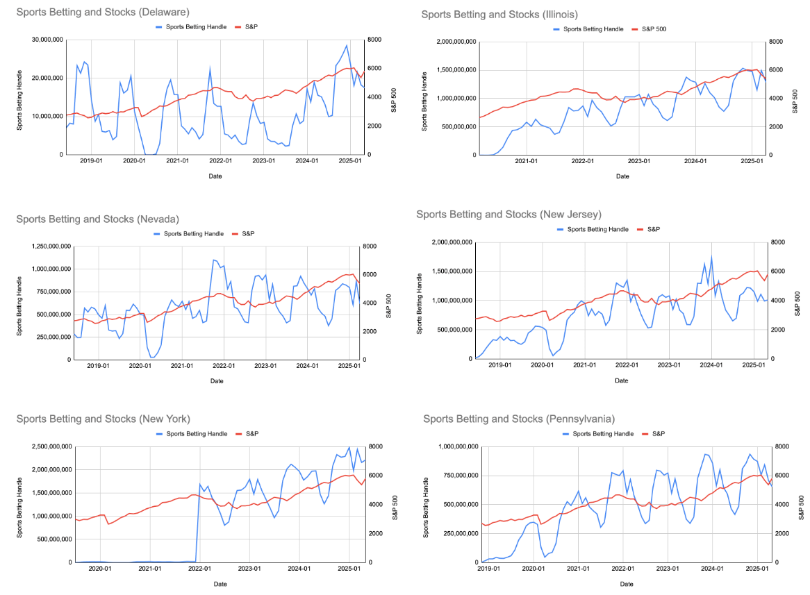
Upon initial examination of sports betting handle and S&P over time (Figure 2), I noticed cyclical patterns and rapid growth in the handle, though no clear correlation was apparent.
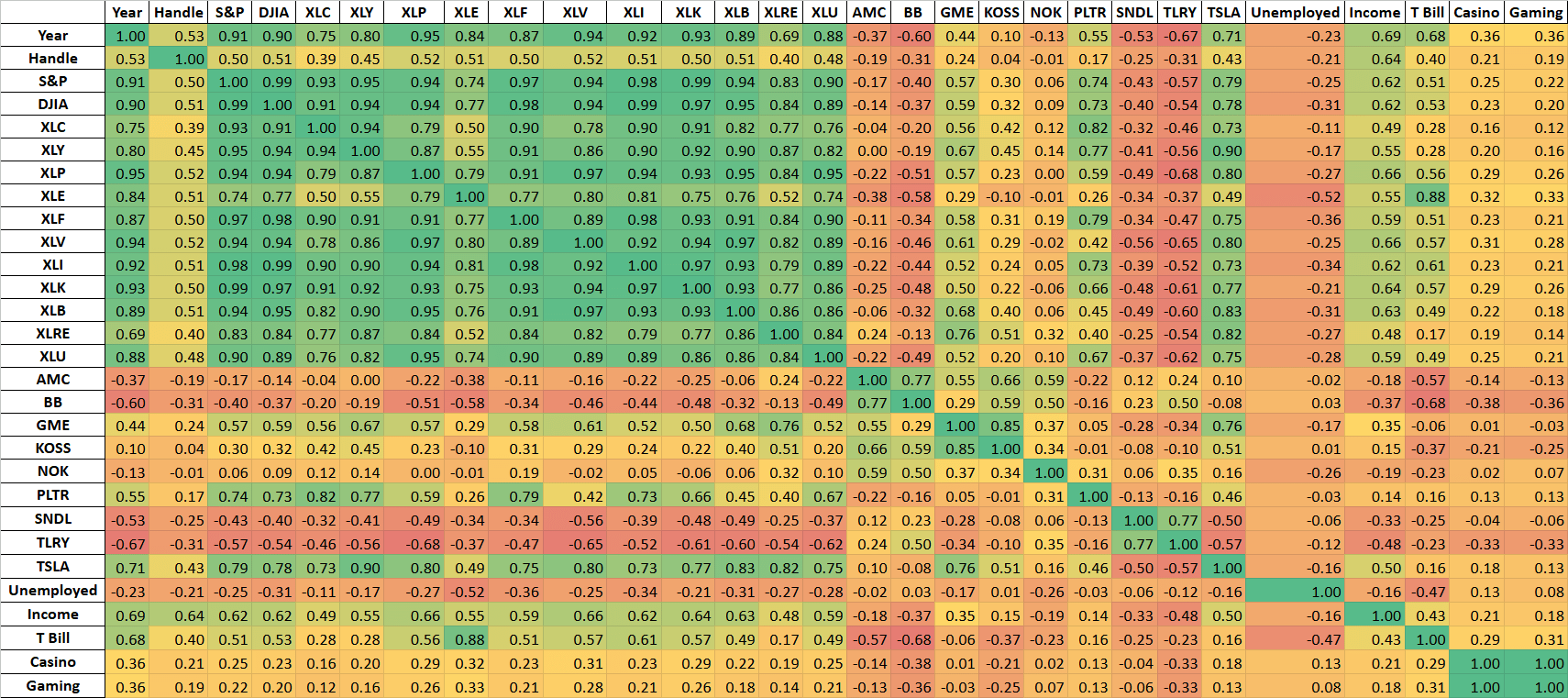
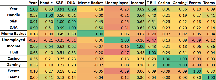
I then proceeded with the analysis by constructing a set of correlation heatmaps with the intention of visualizing linear associations across the dataset. An initial “raw” heatmap was first created that included all variables in the dataset (Figure 3), followed by a filtered version that combines or removes predictors exhibiting high collinearity (Figure 4)—for example, individual meme stocks are aggregated into a single meme stock basket that measures Volume-Weighted Average Price (VWAP). The heatmaps revealed moderate levels of correlation between sports betting handle and broad market indices, as well as significant multicollinearity between financial variables.
Elastic Net regressions using the variables from the filtered heatmap were employed as a diagnostic tool for addressing multicollinearity. By performing feature shrinkage to collinear predictors, Elastic Net reduces instability in coefficient estimates. However, because Elastic Net was unable to account for autocorrelation, the results were not used for final inference, but rather to guide variable inclusion and final model specification. Additionally, variance inflation factors (VIFs) were computed as another diagnostic for multicollinearity.
Finally, the variables highlighted by the Elastic Net regression were used to run state-level GLSAR regressions to account for the serial correlation that affected each state. This multi-stage methodology allowed a structured examination of the co-movement of sports betting handle with the S&P and other contextual factors while addressing multicollinearity, temporal dependence, and robustness to early post-legalization dynamics.
In my analysis, key conceptual variables have been operationalized with observable market behavior. For example, changes in aggregate sports betting activity are used to measure risk seeking behavior, with increases in monthly sports betting handle being interpreted as showing higher levels of risk seeking. Risk perception is also proxied using stock market performance, specifically broad indices like the S&P 500, where downturns are assumed to bring individuals below their reference point and alter perceived risk, which is consistent with Prospect Theory. Finally, exposure to betting opportunities is represented by the index of state-month indicators for major sporting events, team participation, and number of games. Macroeconomic conditions are also captured by labor market metrics and price indices.
Hypotheses
Before analyzing the data, I state the hypotheses grounded in Prospect Theory4, which predicts that when individuals experience losses relative to a reference point, they exhibit increased risk seeking behavior. Applied to the context of financial markets and sports betting, this theory suggests that downturns in the stock market may increase the likelihood of individuals to engage in risky betting behavior by putting them in the loss domain.
H1: Periods of weaker stock market conditions—implying realized or perceived losses—are associated with higher levels of sports betting activity, consistent with the idea of increased risk seeking behavior when individuals are closer to or within the loss domain.
H2: Periods of high speculative sentiment in equity markets, proxied through meme stocks, see higher sports betting handle as a function of risk appetite.
Betting Handle and Stock Market Over Time
Figure 2 shows the sports betting handle over time on the left vertical axis and the value of the S&P 500 over time on the right vertical axis in each of the six chosen states. Graphs were constructed to visualize co-movement of betting handle with the S&P—which was chosen as the primary measure of stock market performance. The first thing to notice about the lines for sports betting handle is that most of them follow a cyclical pattern where they peak around September to January and reach their minimum during June or July. The patterns seem to generally follow the NFL, which runs from September to February, and this makes sense as NFL football is the most bet-on sport in the US33. In addition, the NBA also runs from September to June and the MLB playoffs take place in October, which also explains this cyclical pattern. Sports betting handle also increases rapidly, especially in early transitional periods where growth resembles an exponential pattern. This rapid growth is especially pronounced in relatively later adopters such as Illinois and New York.
Just by looking at the graphs, no clear correlation is visible between the two variables. However, although these time series graphs alone cannot offer insight on how the predictors interact, they help characterize the data and identify confounding factors such as the seasonality of sports betting that I will address with exposure variables described in section “Selection of Events (Exposure Variables)” and the discrepancy of national level stock data versus state level sports betting data—as the latter would be affected by state level income or unemployment that I used as predictors to normalize the data points.
Correlation Heatmaps
The first step in analyzing the relationships between sports betting handle and the set of variables was to construct correlation heatmaps, allowing me to visualize linear associations across the dataset. The heatmaps serve a descriptive purpose by showing patterns of co-movement and providing insight into potential multicollinearity between my predictors. In this section, I present two sets of correlation heatmaps: an initial one with the entire dataset and a filtered one that combines or removes highly collinear variables. Each set consists of one heatmap that includes all observations and one that excludes observations within six months post-legalization.
Raw Heatmap
Figure 3 shows the initial heatmap consisting of all variables and using all observations. Major indices like the S&P and sector-level SPDR funds exhibit high correlations, reflecting their shared exposure to broad market movements. This suggests significant collinearity between the financial market variables, indicating that including all of them would introduce multicollinearity without adding independent explanatory power.
Compared to the major stocks and indices, the meme stocks exhibit weaker correlations in both directions, likely reflecting idiosyncratic sentiment shocks and episodic trading frenzies of the meme stocks rather than stable movement that aligns with the indices. Despite varying degrees of correlation, the meme stocks themselves form a cluster that is internally correlated, motivating the use of a meme stock basket to capture speculative sentiment and minimize multicollinearity.
The highest magnitude correlations with sports betting handle are seen for the average annual personal income by state (r=0.64) and the secondary market rate of the US 3-Month Treasury Bill (r=0.40). A low negative correlation is also observed between the state unemployment rate and the handle (r=-0.21). Such results accord with expected economic intuition: states in which more residents are employed and have higher income will generate a larger gross amount of sports betting handle flow. Thus, these variables serve as useful controls for both national and state level economic conditions.
Figure A1 (Appendix A) reproduces this initial correlation heatmap with observations within six months of legalization excluded, demonstrating that such trends are not driven by transitional dynamics.
Variable Reduction and Aggregation
Following review of the initial heatmap, variables were removed or combined to address issues of multicollinearity, serial correlation, and redundancy among predictors.
First, the 11 Select Sector SPDR Funds were removed based on their extreme collinearity with each other, as well as with the S&P 500 and the Dow Jones.
Second, individual meme stocks were aggregated into a composite meme stock basket that measured volume weighted average price (VWAP). For the regression analyses, this basket was narrowed down to four: GME, AMC, PLTR, and SNDL. The selections for this final basket were based on the average daily absolute percent change in trading volume, which was used as a proxy for retail-driven trading activity motivated by Internet hype. I posit that large changes in volume often reflect trading driven by social media attention and not traditional valuation models44. Besides this measure of volatility, I also took the continuity of fluctuating patterns into account, with the final four meme stocks covering a diverse range of industries and reflecting meme-driven volatility. Although social media mentions are a direct measure of attention, this data is difficult to aggregate in a consistent manner on a monthly basis. Therefore, I use large and persistent deviations in trading volume as a proxy for retail-driven trading activity that is motivated by sentiment. Volume-based measures not only proxy the effects of online attention but also the translation of this attention into actual trades, which is the mechanism of interest in the context of spillovers into betting behavior. This is in line with literature on meme stocks and retail speculation, which typically focuses on abnormal volume and volatility as a proxy for hype-driven trading activity.
Third, two continuous measures of exposure replaced the set of event-specific categorical indicators for individual sporting event types: the Total Teams variable was defined as the total number of teams from a given state involved in any of the eight chosen events during a given month, and the Total Events variable was defined as the total number of games played by those teams across all eight chosen events during a given month.
Filtered Heatmap
A filtered correlation heatmap (Figure 4) to guide final variable inclusion in subsequent regression models was generated using the reduced set of predictor variables described in the previous section. Variables were generally prioritized for final inclusion if they exhibited high correlation with sports betting handle and low serial correlation, measured by correlation with year.
Several variables remained as exceptions to these rules of exclusion based on either conceptual significance or favorable statistical properties. First, Total Events and Total Teams were retained due to low correlation with year and importance in explaining short and mid-term perturbations from long-term betting handle trends. Despite a high correlation with year, S&P 500 was kept to measure stock market movements, and because of its medium correlation with handle. Average Annual Personal Income was also retained due to its high relevance to macroeconomics and because it had the highest correlation with handle (r=0.64) in spite of serial correlation—the benefits of this factor outweigh its cost and serial correlation will be addressed through the use of state-specific GLSAR. Finally, the Unemployment Rate was kept as an additional relevant macroeconomic factor to capture cyclical economic changes that could influence discretionary gambling, as its correlation with time was relatively low.
The final set of variables retained for the empirical analysis were as follows: Average Annual Personal Income, Total Events, Total Teams, Unemployment Rate, and S&P 500. In addition, state fixed effects were included as variables with Delaware being the base case.
Figure A2 (Appendix A) shows the version of this filtered heatmap with the first six months excluded, once again showing that core trends remain stable without the transition period.
Shortcomings of Correlation Heatmaps
Although correlation heatmaps can present basic linear dynamics between variables, Pearson correlation is a first-pass diagnostic tool and does not provide strong enough evidence to draw conclusions about the effect of each predictor on betting handle, as it does not account for confounding factors. However, these heatmaps play the important role of visualizing potential collinearity between predictors, which motivates the need for regressions discussed in sections “Variance Inflation Factors (VIFs) and Elastic Net Regression” and “GLSAR Regression,” as well as giving a glance at how the predictors move in relation to each other. Although it cannot show definitive results, correlation analysis in conjunction with the time series graphs presented in section ”Betting Handle and Stock Market Over Time” provides clear evidence that, post-legalization, the size of the sports betting market has grown steadily alongside the fundamentals of the US economy and that my dataset reliably captures these dynamics.
Variance Inflation Factors (VIFs) and Elastic Net Regression
In order to assess the stability of the models, as well as the presence of multicollinearity indicated by the heatmaps, I ran a series of Elastic Net regressions with varying regularization parameters (α ∈{1,10,100,1000,10000}) using the set of variables derived from the filtered heatmap and holding the mixing parameter constant, which the model uses to split the penalty term equally between L1 (Lasso) and L2 (Ridge) regularization. Thus, the model that the Elastic Net regression implements is well suited for situations with correlated predictors, as the model stabilizes the coefficient estimates without forcing sparsity45. In particular, the coefficients are not completely forced to zero, which demonstrates the shared signal among and correlation of predictors rather than sparsity. Various levels of the penalty were also tested to ensure that the model was not overfitting due to arbitrary regularization choices.
Elastic Net VIFs
Table 1 shows the VIFs that were calculated for each of the chosen regressors. Aside from the state indicator variables, Average Annual Personal Income (≈5.0) exhibited the highest VIF, which suggests moderate multicollinearity driven by shared macroeconomic trends. The S&P 500 (≈2.4) exhibited a relatively low VIF, indicating that much of the multicollinearity in broad market movement was accounted for with removal of the SPDR Funds and DJIA.
The exposure variables, Total Teams (≈3.5) and Total Events (≈1.5), displayed low VIFs which indicates low levels of redundancy with the other final covariates. Taken together, these VIFs do not indicate severe levels of multicollinearity, though they reflect common movement among macroeconomic conditions over time, particularly income. These temporal dependent coefficients are later addressed with GLSAR regression.
VIFs for the α=1 specification and restricted sample are shown in Table A1 (Appendix A) and confirm the trends discussed above.
| Variable | VIF |
|---|---|
| New York | 5.567201474 |
| Average Annual Personal Income | 5.031414556 |
| New Jersey | 3.59412585 |
| Total Teams | 3.538067085 |
| Pennsylvania | 3.020394349 |
| Illinois | 2.511247902 |
| S&P | 2.414342123 |
| Nevada | 1.756000946 |
| Total Events | 1.493220435 |
| Unemployment Rate | 1.321053286 |
Elastic Net Alpha Selection and Coefficient Behavior
Table 2 shows R2 values and coefficients for each value of α when the full sample is used. Model performance as measured using in-sample R2 declines monotonically as α increases, with the specification α=1 consistently achieving the highest explanatory power and larger values of α resulting in substantial underfitting—R2 approaching zero or even becoming negative. This pattern indicates that higher regularization levels lead to an excessive restriction on the parameter space, suppressing economically meaningful variation rather than removing noise. Accordingly, α=1 represents the appropriate bias-variance tradeoff for this analysis.
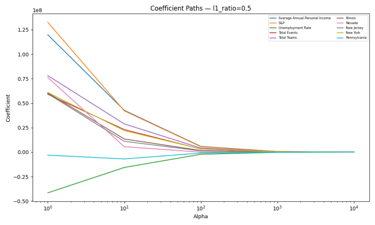
Figure 5 shows the movements of coefficients across different values of α with the full sample used. Coefficient estimates were not found to have collapsed to zero even at high penalty levels, instead shrinking proportionally across predictors while retaining their relative magnitudes. This behavior aligns with existing theory showing that in the presence of correlated regressors, Elastic Net tends to retain groups of related variables rather than selecting a sparse subset45,46. In the context of this study, sporting event exposure measures, macroeconomic indicators, and market variables exhibit co-movement that implies dense signal structure rather than sparsity. Thus, the lack of zeros among the coefficients should be taken as evidence of shared explanatory content across covariates rather than a failure of regularization. Additionally, VIF analysis shows that multicollinearity is not substantial with the reduced variable set.
R2 values and coefficient estimates for the restricted sample are reported in Table A2 (Appendix A), which closely mirrors Table 2. Figure A3 (Appendix A) plots the coefficient paths for the restricted sample and resembles Figure 5, reinforcing the choice of α=1.
Based on the results, α=1 is adopted as the reference specification for diagnostic purposes. Elastic Net has been used here to evaluate coefficient stability and multicollinearity rather than as a final estimator. Final inference for my study was conducted using GLS-based models, with variables (section “Filtered Heatmap” above) that are justified by the results of the Elastic Net regression with α=1, VIF diagnostics, and economic interpretability.
| Alpha | R2 | Average Annual Personal Income | S&P | Unemployment Rate | Total Events | Total Teams | Illinois | Nevada | New Jersey | New York | Pennsylvania |
|---|---|---|---|---|---|---|---|---|---|---|---|
| 1 | 0.5161094113 | 119847068.2 | 132639833.5 | -41610796.27 | 59020995.6 | 78156206.18 | 60501938.4 | 76235638.95 | 59638020.1 | 61004334.08 | -3085160.935 |
| 10 | 0.2525202022 | 42668629.12 | 42132312.05 | -15668848.5 | 23004412.8 | 28782023.66 | 13387966.45 | 5528766.098 | 11018293.8 | 21900499.66 | -6960694.571 |
| 100 | 0.03622808084 | 5811544.59 | 5503452.104 | -2193532.81 | 3156115.484 | 4077464.558 | 1642475.134 | 19649.68374 | 1277267.326 | 3202167.165 | -948280.9091 |
| 1000 | -0.0001158376803 | 603474.9413 | 568298.5154 | -228439.0031 | 327803.1881 | 425798.892 | 168420.939 | -7090.743889 | 130025.7451 | 335641.4004 | -97919.0297 |
| 10000 | -0.003989832188 | 60579.90763 | 57015.73539 | -22937.9728 | 32906.60833 | 42768.65585 | 16884.55471 | -804.4993096 | 13025.40923 | 33725.49211 | -9822.560464 |
Elastic Net Predicted vs Observed and Residuals
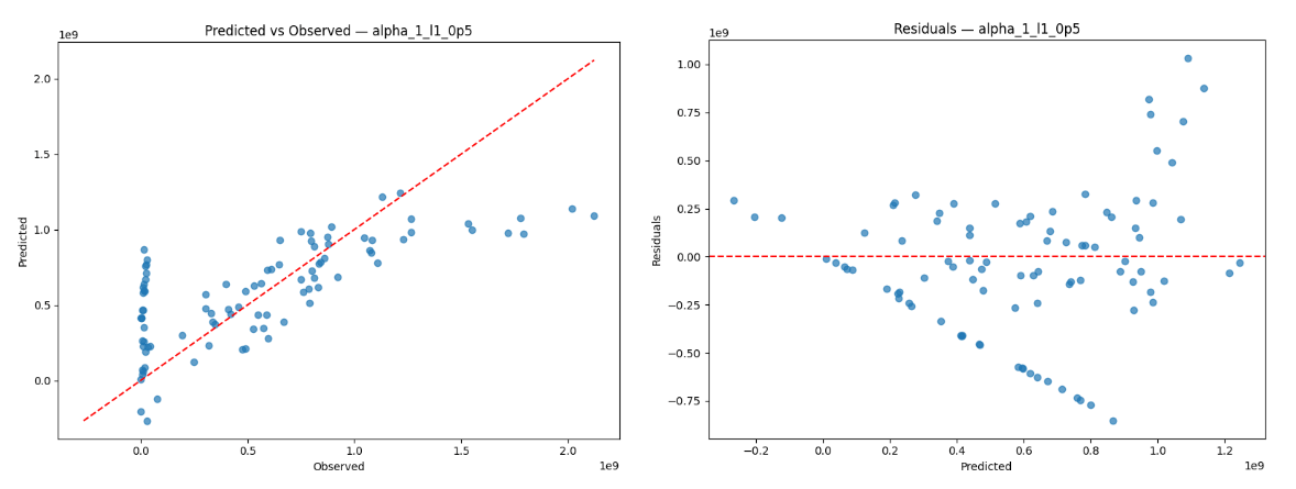
Figure 6 (left) shows the observed values for sports betting handle against the values for sports betting handle predicted by Elastic Net using the α=1 specification and full sample. The plot for predicted-vs-observed handle values shows a positive association and clustering observations around the 45 degree line at moderate handle values, which suggests that the model is relatively accurate at predicting values in the central range of the data. However, the model overpredicts at low handle values, which may be due to serial correlation in sports betting handle. It also underpredicts handle at higher values, though this is consistent with shrinkage imposed by the Elastic Net regularization that dampens extreme values despite the presence of strong signals.
Figure 6 (right) shows the corresponding residuals from the α=1 specification and full sample. The residual plots help us visualize this trend through a different lens, as residuals remain near zero for the center range of the data. However, the heteroskedastic pattern as betting handle value rises is apparent in the residual plot as well, indicating that Elastic Net experiences decreased predictive power at large spikes in sports betting activity, which may reflect nonlinear dynamics and the episodic nature of betting. The serial correlation is apparent as well, likely due to the fact that time series data points are dependent on past points46. In addition, 131 observations in the dataset have a handle value under  813 million. As a result of such exponential growth and the use of a linear model, the scale of the y-axis makes values that are just a one or two orders of magnitude lower look extremely small, even if they are not proportionally as small on an exponential scale. The halting of sporting events during the COVID-19 pandemic may have also caused a drop in sports betting.
Aside from serial correlation, residuals generally exhibit homoskedastic behavior, along with an R2 value at α=1 that indicates a moderately positive linear relationship. The behavior of the residuals is consistent with my intention for the role of Elastic Net in this analysis, where I stabilize coefficient estimation with multicollinearity despite not fully explaining behavior. The tendency to underpredict extreme outcomes again serves to confirm that Elastic Net is too conservative for final inference, especially when a significant degree of economic variation is captured in high-handle observations.
These results taken together support the use of the α=1 Elastic Net approach as an indicative benchmark of variable relevance and stability of coefficients. As seen in Figures A4 and A5 (Appendix A), predicted values are progressively more compressed toward the mean as values for α get larger, implying that predictive power decreases when α>1. This pattern remains unchanged when the first six months are excluded, as shown in Figures A6 and A7 (Appendix A), showing that this trend is not driven by early transitional volatility.
However, these findings also point to the necessity of moving on to state-specific GLS-based models that are able to capture more sophisticated dynamics and regional disparities as well as addressing serial correlation without reducing the pool of significant covariates proposed by the preceding Elastic Net approach.
GLSAR Regression
As a final step, state-level GLSAR regressions with a trend function were estimated to address serial correlation and for final inference. Each state was modeled separately using the set of variables from the Elastic Net model, focusing on within-state dynamics rather than comparisons across states.
GLSAR R2 Summary
Table 3 shows the R2 values resulting from the state-level GLSAR models on the full sample. R2 values shown in the table suggest that the model specification holds substantial explanatory power of variation in betting handle across most jurisdictions. All states except for Delaware exhibit high R2 values in both full and restricted sample regressions (around 0.72 to 0.86), reflecting stable regulatory environments where the largest sources of variation are captured by the covariates.
However, Delaware exhibits significantly lower R2 values (0.39 and 0.42), although this is best understood in the context of institutional conditions and not weak model performance. Delaware operates a state-controlled lottery framework with limited operator participation, which results in lower betting handle variance. When the dependent variable exhibits low variance as in the case of Delaware, explanatory power is mechanically constrained47. For the other states, the lack of structural breaks allow a static GLS specification to capture the majority of variation source. From an economic perspective, this means that even statistically significant variables have limited power in a highly regulated market.
Because variations in R2 reflect differences in market maturity, regulatory design, and betting market transitional dynamics rather than poor model validity, the primary specification is retained to preserve cross-state comparability and avoid overfitting. Robustness checks confirm that substantive conclusions remain unchanged across alternative sample restrictions. Table A3 (Appendix A) reports the state-level R2 values obtained from the restricted sample, which resulted in conclusions that are consistent with the full sample specification.
| State | R2 |
|---|---|
| New York | 0.8552 |
| New Jersey | 0.7718 |
| Pennsylvania | 0.7579 |
| Illinois | 0.8397 |
| Delaware | 0.3896 |
| Nevada | 0.7496 |
GLSAR Predicted vs Observed and Residuals
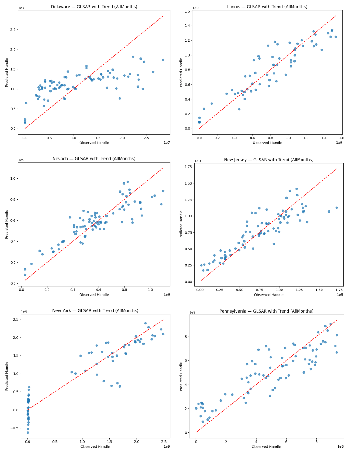
Figure 7 shows the predicted-vs-observed scatter plots of sports betting handle value for the state-level GLSAR models on the full sample. The figure provides further evidence that the model captures most sources of betting handle variation and they reveal differences in market structure and transitional dynamics across states. As discussed above, the model holds strong prediction accuracy for New Jersey, Nevada, Illinois, and Pennsylvania, as observations gather mostly along the 45 degree line. From an applied perspective, this indicates that the included covariates are accounting for the key drivers of sports betting handle in mature markets. Deviations increase slightly as true betting handle increases, but this reflects scale effects and exponential growth in betting handle rather than heteroskedasticity.
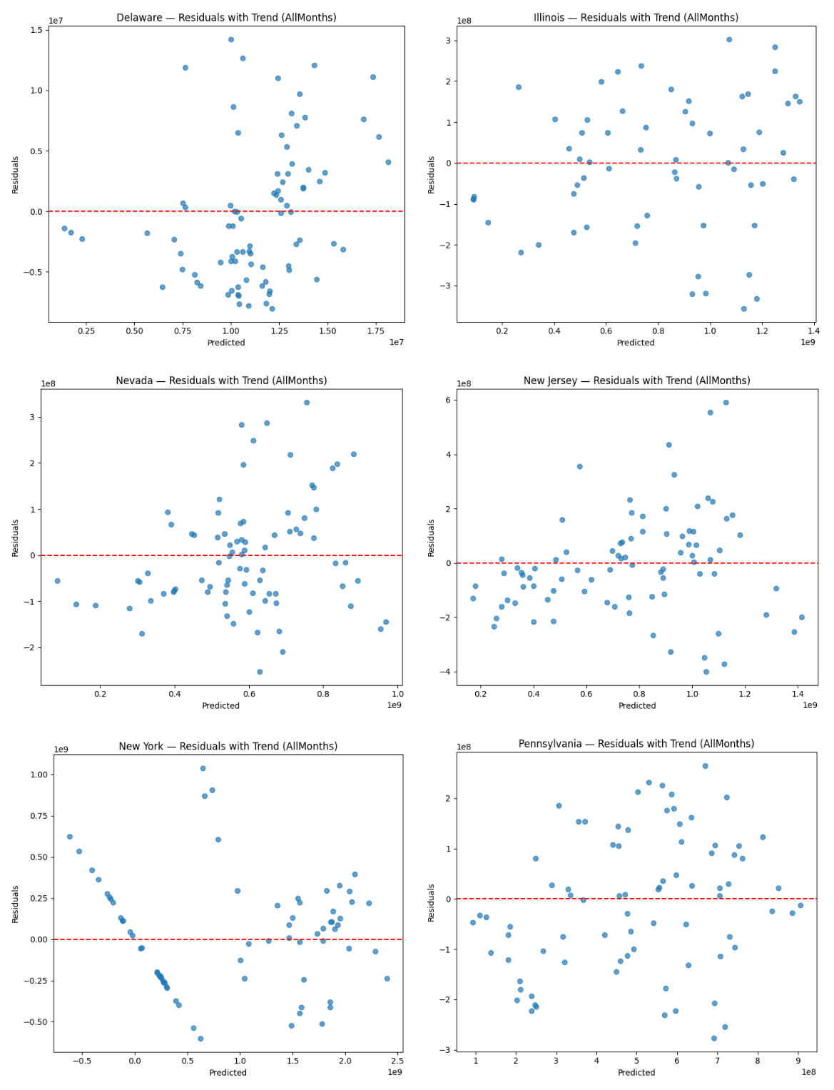
Figure 8 shows the corresponding residuals. The residual plots tell the same story for those four states and largely approximate white noise. They center around zero and lack any clear nonlinear patterns, providing evidence that linear form is appropriate for stabilized markets. Importantly, none of these states display any curvature or sustained trends in the residuals, supporting the appropriateness of a static specification for mature markets. This is consistent with the behavioral model, where sports betting is proportional to changes in exposure and market conditions in mature markets.
Despite its high R2 value, New York displays serial correlation in its residual plots that reflects rapid post-legalization expansion, high promotional intensity, and path-dependent growth following the mobile launch in January 2022. GLS models correct for heteroskedasticity and contemporaneous correlation but do not fully account for dynamic adjustment without an autoregressive structure48. This implies that although the model explains overall variation well, the short-run behavioral responses of newly liberalized and high-liquidity markets may have dynamic features beyond the static specification.
As shown in the previous section, Delaware stands apart from the other states with predicted handle values being compressed around the mean, matching the state’s low R2 value. Econometrically, this represents a market where institutional constraints dominate individual behavioral responses, effectively constraining the impact of changes in the covariates. Such a pattern exemplifies the highly regulated low-variance betting market in Delaware, which causes covariates to have limited explanatory leverage—they cannot account for all observed variation as changes in the values of covariates translate into only small changes in predicted handle.
Figures A8 and A9 (Appendix A) display similar plots for the GLSAR models done on the restricted sample, reinforcing the interpretation presented in this section.
GLSAR p-values and Coefficients
Table 4 contains the p-values, coefficients, and confidence intervals from the state-level GLSAR regressions with a linear time trend using the full sample.
Across all six states, the Constant value was statistically significant (p<0.05), symbolizing the baseline demand in sports betting in each state when covariates are held to zero. This could be due to factors such as initial marketing influence from advertising or existing inclination to sports betting.
Total Events and Total Teams showed positive coefficients for every state. Additionally, Total Events exhibited p-values that were statistically significant at the 95% confidence level for all states except for New York; Total Teams was significant for all states except for New York and Delaware. This indicates that the increase in exposure to sporting events and availability of betting opportunities have a meaningful impact on betting handle variation, which is reflected in their moderately low to high coefficient values ranging from β=1.27e4 (Delaware Total Teams) to β=8.38e7 (Nevada Total Teams), which are economically and statistically significant.
In all six states, Unemployment Rate and Average Annual Personal Income exhibited p-values that were not statistically significant, suggesting that short-run changes in labor market conditions and income levels have little economic and behavioral significance on sports betting activity in isolation. This may be partly driven by the low costs of engaging in sports betting, allowing sustained betting behavior despite modest fluctuations in personal income or labor conditions. Moreover, macroeconomic factors may still indirectly affect betting behavior in the longer term or through exposure to betting opportunities.
The role of financial market performance differed by state, with the S&P 500 being statistically insignificant in most states. However, New York remained a notable exception to this trend: a statistically significant negative association was observed between the size of the betting handle and the S&P 500 variable (β ≈-3.3e8, p≈0.03) in New York. The negative sign and large magnitude of this coefficient indicate that stock market declines coincide with large increases in aggregate betting activity. This is consistent with my hypothesis that risk seeking behavior would intensify when stock market dips put individuals in the loss domain. From a behavioral perspective, this indicates that financial losses may be associated with increased participation in recreational risk-taking activities such as sports betting in large markets. However, the fact that this relationship is found in New York but not elsewhere suggests that state-specific factors could be important in explaining how financial market conditions relate to betting behavior. For example, factors related to exposure to or participation in the equity markets could be important, though these mechanisms are not explored in this study and are left for future research.
A pattern emerges when analyzing the linear time trend across states. In New York and Illinois, the trend coefficient is statistically significant and positive, which implies that the long-run growth path cannot be fully explained by covariates such as events or economic conditions. It’s worth noting that these states are large and have relatively later legalization dates, suggesting that the trend captures genuine structural growth and is statistically and economically meaningful47. By contrast, the states of Pennsylvania, New Jersey, and Nevada exhibit insignificant trend coefficients despite their high R2 values, indicating that long-run variation in these states can be explained by the other regressors that evolve smoothly over time and absorb low-frequency changes in the betting market. From an econometric standpoint, the trend may still play an important role, although its significance is lost due to competition with other regressors49. A distinct case of the trend coefficient is seen in Delaware, which has an insignificant trend and a much lower R2 value than the others, reflecting limitations of the data rather than model failure. Delaware’s betting market is much smaller compared to the other five states, making it subject to higher volatility and discrete shocks. As a result, neither a smooth trend nor observed covariates can explain handle variation reliably, which is typical in short time series dominated by noise50.
Importantly, a statistically insignificant trend may still contribute to model fit, as the trend component controls for low-frequency levels in the residuals and reduces serial correlation while ensuring that other regressors are not implicitly being used as proxies for trend growth. Its use can still be important to ensure coefficient stability and R2 by ensuring that the correct amount of variation is captured between long and short run, which is important for the GLS model where spurious correlation can occur unless modeled, inflating residual variance49. Therefore, genuine variation appears in the trend significance that corresponds with market maturity, volatility, and growth mechanism differences between states. The fact that the trend improves model performance even while insignificant suggests that it is performing its expected function as a key econometric control rather than a forced explanatory variable47, 50.
Coefficient estimates, p-values, and confidence intervals for each state-level GLSAR regression with observations within six months of legalization excluded are reported in Table A4 (Appendix A), which show robustness.
| Variable | Coefficient | P_Value | CI_Lower | CI_Upper |
|---|---|---|---|---|
| DELAWARE | ||||
| const | 1.12E+07 | 1.08E-08 | 7.75E+06 | 1.47E+07 |
| S&P | 2.67E+06 | 3.14E-01 | -2.58E+06 | 7.93E+06 |
| Unemployment Rate | -3.82E+05 | 6.33E-01 | -1.97E+06 | 1.20E+06 |
| Total Events | 2.25E+06 | 8.28E-06 | 1.31E+06 | 3.19E+06 |
| Total Teams | 1.27E+04 | 9.70E-01 | -6.69E+05 | 6.94E+05 |
| Average Annual Personal Income | -2.56E+05 | 8.85E-01 | -3.77E+06 | 3.26E+06 |
| Trend | -1.26E+06 | 7.14E-01 | -8.11E+06 | 5.58E+06 |
| ILLINOIS | ||||
| const | 8.08E+08 | 1.99E-21 | 7.03E+08 | 9.13E+08 |
| S&P | -3.67E+07 | 6.40E-01 | -1.93E+08 | 1.20E+08 |
| Unemployment Rate | 9.28E+06 | 7.31E-01 | -4.45E+07 | 6.30E+07 |
| Total Events | 5.18E+07 | 1.18E-02 | 1.20E+07 | 9.16E+07 |
| Total Teams | 4.60E+07 | 1.09E-02 | 1.11E+07 | 8.10E+07 |
| Average Annual Personal Income | 3.06E+07 | 5.82E-01 | -8.01E+07 | 1.41E+08 |
| Trend | 3.32E+08 | 5.34E-04 | 1.51E+08 | 5.13E+08 |
| NEVADA | ||||
| const | 5.87E+08 | 6.31E-35 | 5.35E+08 | 6.39E+08 |
| S&P | 6.65E+07 | 2.48E-01 | -4.74E+07 | 1.80E+08 |
| Unemployment Rate | -2.97E+07 | 1.03E-01 | -6.57E+07 | 6.18E+06 |
| Total Events | 5.51E+07 | 1.19E-04 | 2.81E+07 | 8.21E+07 |
| Total Teams | 8.38E+07 | 3.84E-08 | 5.66E+07 | 1.11E+08 |
| Average Annual Personal Income | 7.05E+07 | 1.47E-01 | -2.53E+07 | 1.66E+08 |
| Trend | -2.31E+07 | 7.51E-01 | -1.68E+08 | 1.22E+08 |
| NEW JERSEY | ||||
| const | 7.66E+08 | 2.83E-28 | 6.78E+08 | 8.53E+08 |
| S&P | 1.10E+08 | 2.19E-01 | -6.69E+07 | 2.87E+08 |
| Unemployment Rate | 2.23E+05 | 9.94E-01 | -6.08E+07 | 6.13E+07 |
| Total Events | 6.62E+07 | 9.40E-04 | 2.79E+07 | 1.05E+08 |
| Total Teams | 6.32E+07 | 1.17E-03 | 2.59E+07 | 1.01E+08 |
| Average Annual Personal Income | 1.39E+08 | 5.22E-02 | -1.34E+06 | 2.80E+08 |
| Trend | 4.35E+07 | 7.06E-01 | -1.85E+08 | 2.72E+08 |
| NEW YORK | ||||
| const | 9.54E+08 | 2.22E-14 | 7.61E+08 | 1.15E+09 |
| S&P | -3.30E+08 | 3.01E-02 | -6.28E+08 | -3.28E+07 |
| Unemployment Rate | 2.79E+06 | 9.65E-01 | -1.22E+08 | 1.28E+08 |
| Total Events | 7.10E+07 | 1.11E-01 | -1.68E+07 | 1.59E+08 |
| Total Teams | 5.09E+06 | 9.16E-01 | -9.08E+07 | 1.01E+08 |
| Average Annual Personal Income | 1.88E+07 | 8.69E-01 | -2.09E+08 | 2.46E+08 |
| Trend | 1.12E+09 | 1.82E-07 | 7.39E+08 | 1.50E+09 |
| PENNSYLVANIA | ||||
| const | 5.00E+08 | 1.20E-16 | 4.08E+08 | 5.92E+08 |
| S&P | 4.43E+07 | 4.52E-01 | -7.25E+07 | 1.61E+08 |
| Unemployment Rate | -3.52E+06 | 8.42E-01 | -3.85E+07 | 3.15E+07 |
| Total Events | 2.98E+07 | 1.93E-02 | 4.98E+06 | 5.46E+07 |
| Total Teams | 4.61E+07 | 4.51E-04 | 2.11E+07 | 7.11E+07 |
| Average Annual Personal Income | 3.90E+07 | 3.53E-01 | -4.41E+07 | 1.22E+08 |
| Trend | 1.04E+08 | 1.88E-01 | -5.22E+07 | 2.61E+08 |
Limitations and Discussion
Conclusions of My Study
The findings of this research offer tentative associative evidence of the existence of a relationship between stock market downturns and sports betting, as predicted by Prospect Theory. In the state-level GLSAR models, a statistically significant negative association between the S&P 500 and sports betting handle is found in New York, suggesting that periods of lower equity market performance are linked to higher levels of betting activity. This result is in line with the prediction that individuals who experience losses in relation to a reference point are likely to exhibit risk-seeking behavior, and it is taken as an associative extension of this behavioral pattern from financial markets to recreational gambling rather than a causal effect. Crucially, however, this association is not constant across all states, showing the importance of market structure, development, and institutional factors. The state-specific nature of the results is certainly intriguing and somewhat surprising, and suggests that the results found in New York may not be representative of a general pattern. This variability indicates that the spillover of behavioral associations from financial markets to sports betting is likely to be state-specific and potentially amplified in large financial centers such as New York. One possibility is that in New York, people may be more directly exposed to equity market fluctuations—either through a greater rate of participation in the stock market or through a greater interest in financial news and market fluctuations. As such, the results are consistent with an interpretation that financial and recreational risk-taking are behaviorally associated under certain conditions rather than universally. Future research could explore this dynamic by examining differences in stock market participation, or financial literacy, across states to understand the mechanisms behind the results.
In addition to its main finding, the current research makes several other contributions to the literature on behavioral finance. First, it provides real-world evidence that risk preferences can depend on context and be influenced by perceived financial loss, rather than being fixed or rational. Second, the findings are consistent with the idea that risk behavior can spill over across contexts when people try to recoup losses, especially when they have frequent opportunities to do so. The results also provide potential guidance for real-world policies from the perspective of the recent surge in the expansion of sports betting. If sports betting acts as an outlet for risk-taking during financial crises, then sports betting could become more intense during periods of overall financial stress. This again points to the importance of risk awareness as part of financial education and counseling programs, particularly for retail investors and individuals who may be subject to income or net wealth shocks. With respect to the regulatory framework, gambling platforms may be subject to monitoring sports betting activity during periods of financial stress or implementing safeguards to prevent risk-taking without unduly restricting consumer choice.
The legalization of sports betting creates a new type of empirical setting for investigating reactions to monetary losses beyond traditional financial markets. In revealing the conditions under which the stock market co-moves with sports betting, this research increases the scope of Prospect Theory research and suggests new pathways for research into risk-taking in new types of emerging digital and recreational markets.
Limitations of My Study and Recommendations for Future Research
However, it is important to consider several theoretical and methodological limitations. First, sports betting in the US is a relatively new phenomenon. This means that the time horizon of the analysis is limited. This limits the potential to examine long-term behaviors or structural shifts in the betting markets as they continue to develop. Second, the results of the analysis are not generalizable across the US or other international contexts. This is because the analysis looks at six states in the US that were early adopters of sports betting. While useful in examining mature markets, the economic and regulatory environments in these states may not be representative of the US or international contexts at large.
Third, the use of monthly aggregate state-level data limits the potential to examine individual-level decision-making or within-month behaviors in response to market movements. The exposure variables defined in the analysis of sports events and participation do not capture differences in event or sporting participation popularity or betting intensity. Fourth, although state-level GLSAR models were employed to address the problem of serial correlation, there still existed residual autocorrelation in New York, which might have resulted from rapid expansion in the post-legalization period. Future research might attempt to utilize different structures of autoregressive terms or incorporate higher-order lag terms to capture dynamic adjustment effects in rapidly changing environments. Finally, due to the nature of correlational analysis and limited identifying variation, it is difficult to establish causal effects and pinpoint the exact mechanisms that underlie the relationship between stock market performance and sports betting. While the results support behavioral predictions in accordance with Prospect Theory, they must be regarded as merely associative in nature.
Future studies could help alleviate some of the limitations of the current literature by using individual-level betting data, laboratory experiments, or natural experiments that exploit exogenous events in the financial markets or betting environments. A longer time frame could allow for the examination of changes in behavior as the betting markets become more stable, as well as studies that include a wider range of states or international markets that could help examine the impact of regulatory structures and cultural differences on risk-taking behavior. Second, they could help examine the impact of speculative financial assets, such as meme stocks, as a potential moderating or interacting factor in the relationship between the financial markets and gambling behavior, to help disentangle the similar forms of retail-based risk-taking behavior. Third, they could help expand this framework to other emerging forms of risk, such as lotteries, cryptocurrency, or options, as well as help examine the relationship between individual-level portfolio risk and gambling behavior during times of financial stress. Finally, future research could explore the phenomenon of state-specific results by examining the state-to-state variation in equity market participation, financial literacy, or financial information seeking to refine our understanding of the ways in which financial market volatility affects gambling.
Acknowledgements
I would like to thank Daniel J. Connolly for his invaluable guidance throughout this project. I would also like to thank Brandt Bridges for his helpful feedback on the clarity of this paper.
Appendix A
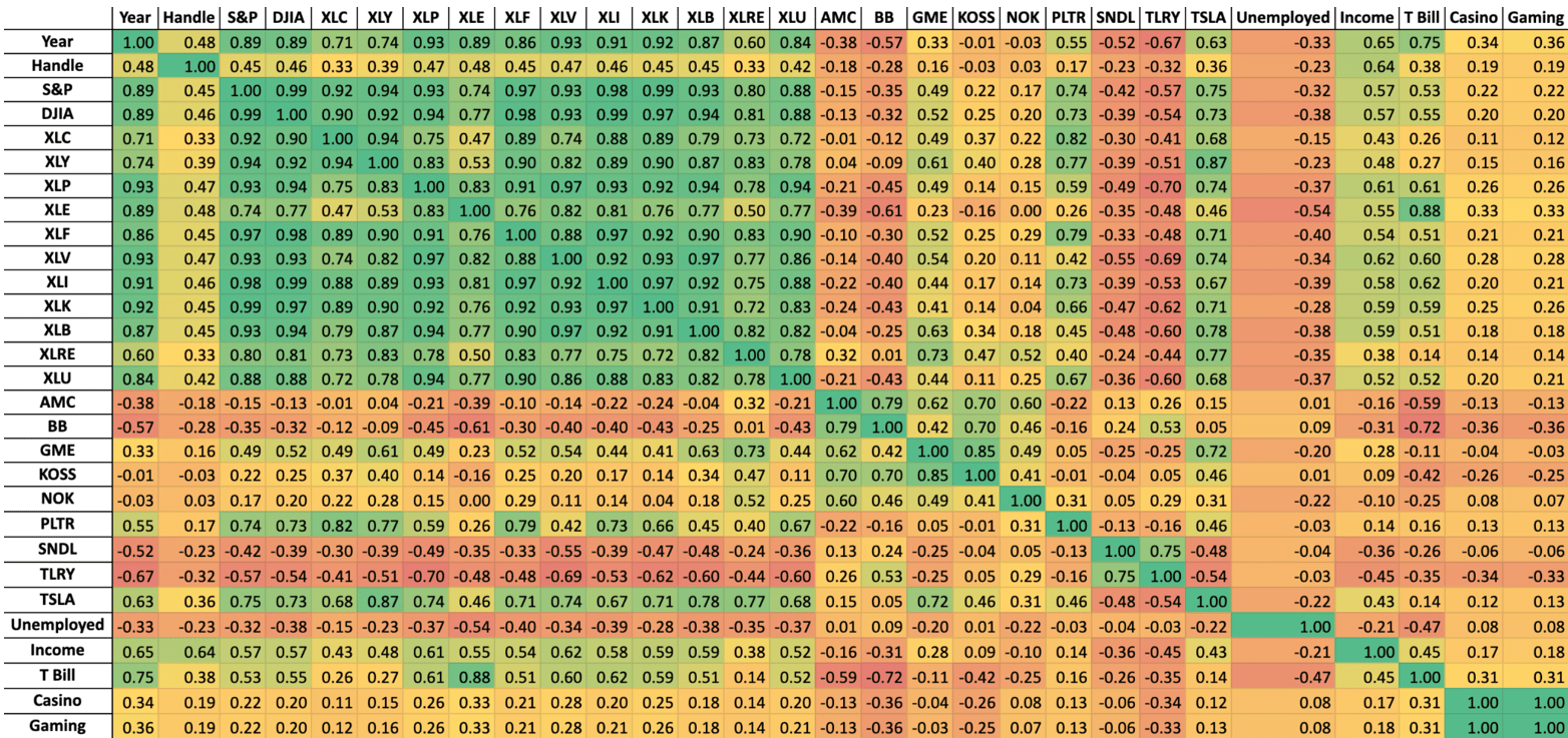
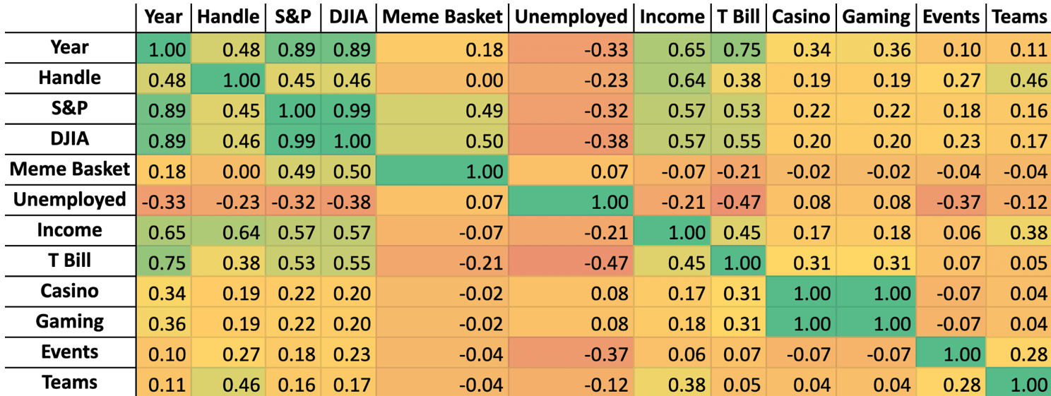
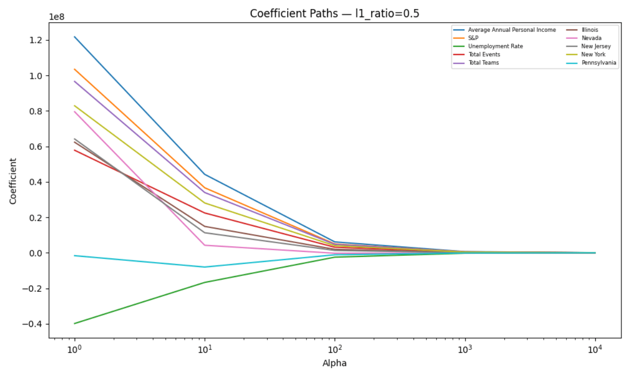
| Variable | VIF |
|---|---|
| New York | 5.750952134 |
| Average Annual Personal Income | 5.434876377 |
| New Jersey | 3.94973844 |
| Total Teams | 3.479410644 |
| Pennsylvania | 3.01523681 |
| Illinois | 2.49474033 |
| S&P | 2.269746944 |
| Nevada | 1.757646912 |
| Total Events | 1.455786282 |
| Unemployment Rate | 1.382122624 |
| Alpha | R2 | Avg. Annual Personal Income | S&P | Unemployment Rate | Total Events | Total Teams | Illinois | Nevada | New Jersey | New York | Pennsylvania |
|---|---|---|---|---|---|---|---|---|---|---|---|
| 1 | 0.5691067084 | 121754794.3 | 103476391.9 | -39887926.95 | 57830411.52 | 96627136.97 | 62367376.12 | 79549162.23 | 64178812.9 | 82904504.39 | -1636430.357 |
| 10 | 0.2545069045 | 44231088.21 | 36663726.17 | -16723078.59 | 22455611.8 | 33992327.48 | 14877931.38 | 4235394.929 | 11295396.32 | 28090381.16 | -8044777.452 |
| 100 | 0.01458092359 | 6128209.982 | 4976740.395 | -2477205.194 | 3113092.368 | 4747267.428 | 1928592.294 | -265433.5911 | 1301699.128 | 3996775.63 | -1139697.085 |
| 1000 | -0.0263419292 | 638000.5364 | 516543.0535 | -259943.718 | 323901.8529 | 495015.3124 | 199339.3069 | -38240.33299 | 132536.4698 | 417614.3914 | -118314.0242 |
| 10000 | -0.03071754242 | 64063.14112 | 51850.60113 | -26122.00743 | 32521.00907 | 49713.87304 | 20000.93819 | -3947.633926 | 13277.36785 | 41949.07824 | -11875.22282 |
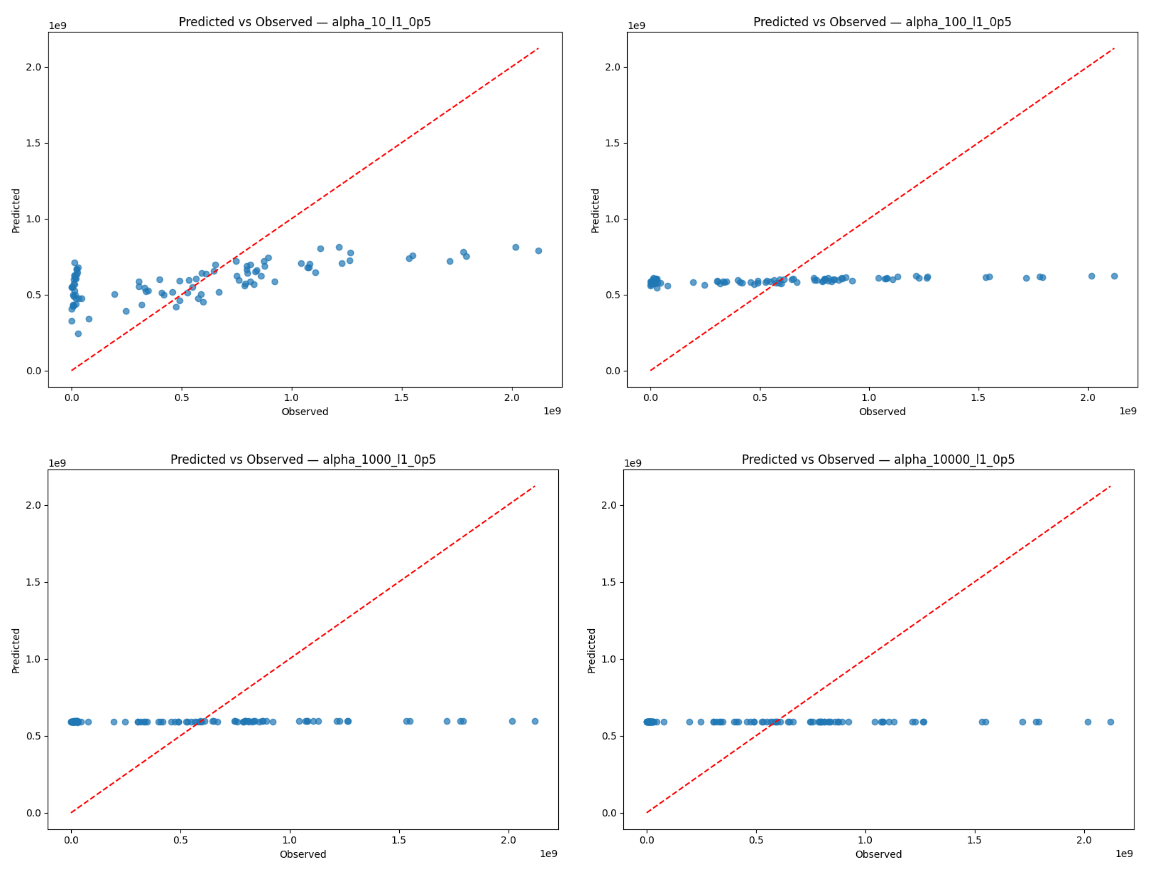
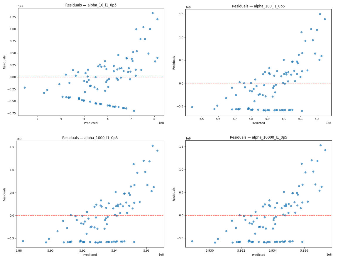
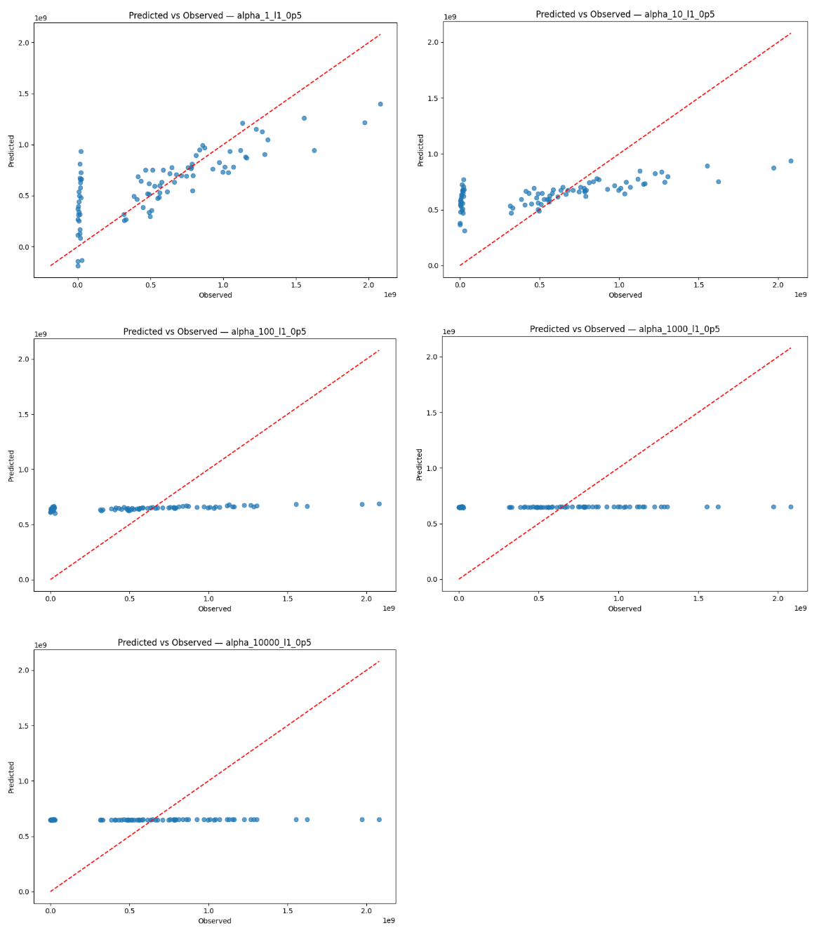
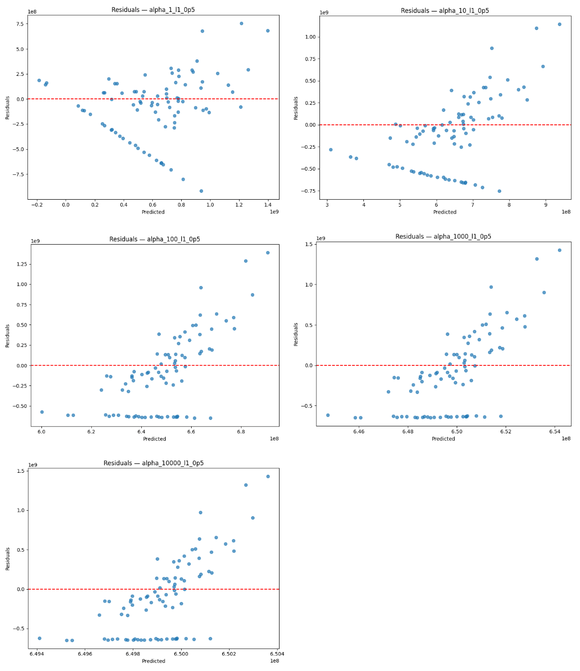
| State | R2 |
|---|---|
| New York | 0.8561 |
| New Jersey | 0.7463 |
| Pennsylvania | 0.7206 |
| Illinois | 0.7525 |
| Delaware | 0.4214 |
| Nevada | 0.7396 |
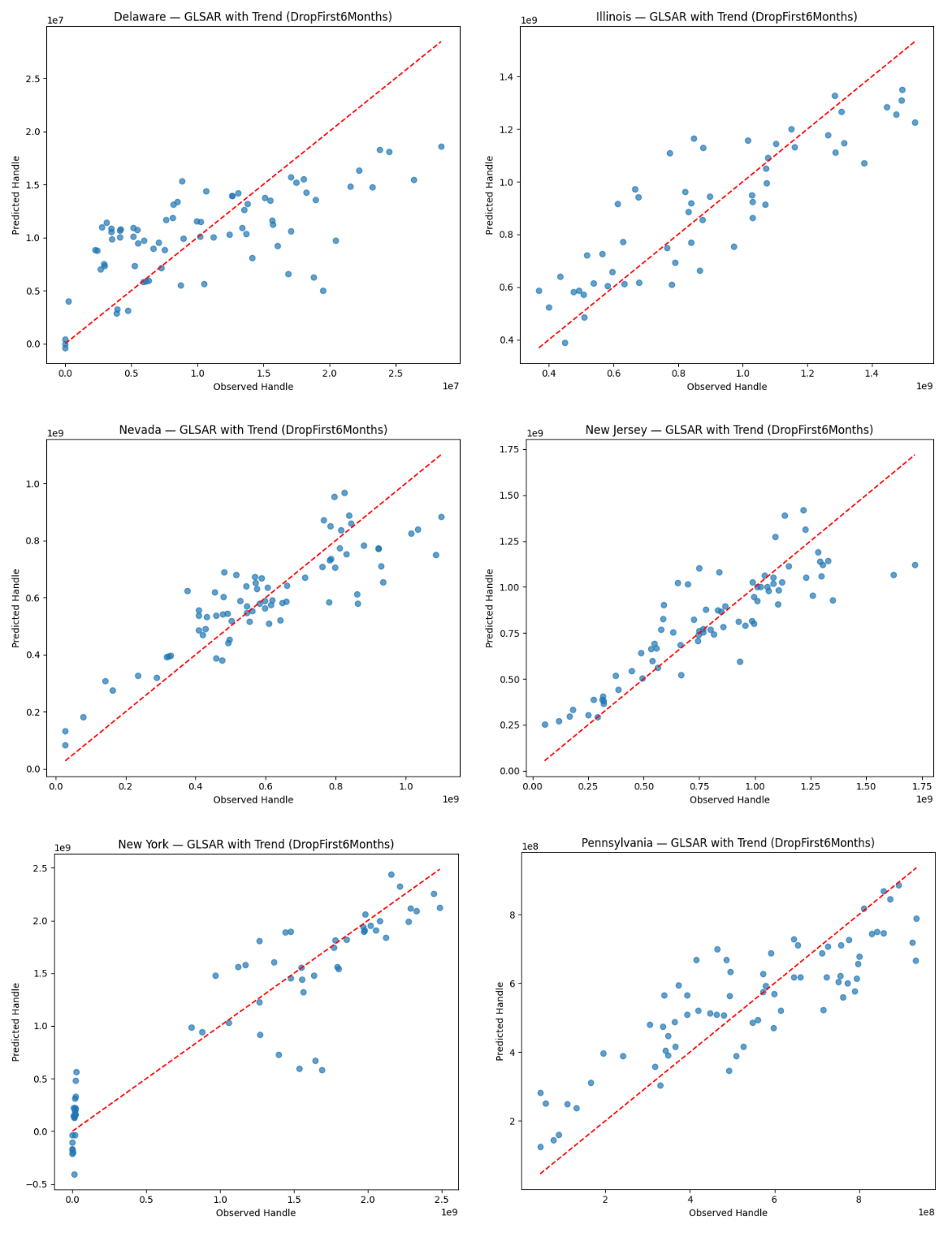
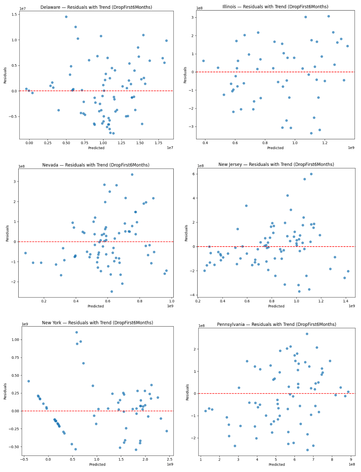
| Variable | Coefficient | P Value | CI Lower | CI Upper |
|---|---|---|---|---|
| DELAWARE | ||||
| const | 1.02E+07 | 2.38E-07 | 6.67E+06 | 1.38E+07 |
| S&P | 1.88E+06 | 4.30E-01 | -2.84E+06 | 6.60E+06 |
| Unemployment Rate | -1.41E+05 | 8.53E-01 | -1.65E+06 | 1.37E+06 |
| Total Events | 2.30E+06 | 2.66E-06 | 1.40E+06 | 3.19E+06 |
| Total Teams | 2.01E+04 | 9.50E-01 | -6.24E+05 | 6.64E+05 |
| Average Annual Personal Income | 2.00E+05 | 9.12E-01 | -3.38E+06 | 3.78E+06 |
| Trend | 9.71E+05 | 7.63E-01 | -5.43E+06 | 7.37E+06 |
| ILLINOIS | ||||
| const | 9.04E+08 | 5.49E-22 | 7.98E+08 | 1.01E+09 |
| S&P | -3.62E+07 | 6.15E-01 | -1.80E+08 | 1.08E+08 |
| Unemployment Rate | 2.70E+07 | 7.39E-01 | -1.35E+08 | 1.89E+08 |
| Total Events | 4.61E+07 | 1.28E-02 | 1.03E+07 | 8.19E+07 |
| Total Teams | 4.29E+07 | 1.31E-02 | 9.41E+06 | 7.63E+07 |
| Average Annual Personal Income | 9.01E+06 | 8.57E-01 | -9.09E+07 | 1.09E+08 |
| Trend | 2.92E+08 | 2.75E-03 | 1.06E+08 | 4.78E+08 |
| NEVADA | ||||
| const | 5.98E+08 | 4.05E-31 | 5.40E+08 | 6.55E+08 |
| S&P | 6.10E+07 | 2.96E-01 | -5.46E+07 | 1.77E+08 |
| Unemployment Rate | -2.92E+07 | 1.39E-01 | -6.82E+07 | 9.68E+06 |
| Total Events | 5.77E+07 | 2.08E-04 | 2.83E+07 | 8.70E+07 |
| Total Teams | 8.29E+07 | 3.31E-07 | 5.37E+07 | 1.12E+08 |
| Average Annual Personal Income | 7.00E+07 | 1.56E-01 | -2.74E+07 | 1.67E+08 |
| Trend | -2.41E+07 | 7.41E-01 | -1.69E+08 | 1.20E+08 |
| NEW JERSEY | ||||
| const | 8.13E+08 | 9.13E-29 | 7.27E+08 | 9.00E+08 |
| S&P | 1.12E+08 | 1.98E-01 | -5.97E+07 | 2.84E+08 |
| Unemployment Rate | 3.09E+05 | 9.92E-01 | -6.44E+07 | 6.51E+07 |
| Total Events | 7.46E+07 | 7.25E-04 | 3.25E+07 | 1.17E+08 |
| Total Teams | 6.98E+07 | 9.01E-04 | 2.97E+07 | 1.10E+08 |
| Average Annual Personal Income | 1.20E+08 | 8.13E-02 | -1.54E+07 | 2.56E+08 |
| Trend | 2.09E+07 | 8.48E-01 | -1.96E+08 | 2.38E+08 |
| NEW YORK | ||||
| const | 1.07E+09 | 1.52E-15 | 8.73E+08 | 1.26E+09 |
| S&P | -3.26E+08 | 2.62E-02 | -6.13E+08 | -4.02E+07 |
| Unemployment Rate | 2.86E+07 | 6.97E-01 | -1.18E+08 | 1.75E+08 |
| Total Events | 7.76E+07 | 1.16E-01 | -1.98E+07 | 1.75E+08 |
| Total Teams | 4.33E+06 | 9.35E-01 | -1.02E+08 | 1.11E+08 |
| Average Annual Personal Income | 3.41E+07 | 7.47E-01 | -1.76E+08 | 2.45E+08 |
| Trend | 1.08E+09 | 3.04E-07 | 7.06E+08 | 1.45E+09 |
| PENNSYLVANIA | ||||
| const | 5.47E+08 | 4.77E-20 | 4.65E+08 | 6.29E+08 |
| S&P | 4.01E+07 | 4.67E-01 | -6.94E+07 | 1.50E+08 |
| Unemployment Rate | -6.57E+06 | 7.31E-01 | -4.46E+07 | 3.14E+07 |
| Total Events | 3.18E+07 | 2.41E-02 | 4.30E+06 | 5.92E+07 |
| Total Teams | 5.08E+07 | 6.40E-04 | 2.25E+07 | 7.90E+07 |
| Average Annual Personal Income | 3.20E+07 | 4.60E-01 | -5.40E+07 | 1.18E+08 |
| Trend | 6.76E+07 | 3.60E-01 | -7.89E+07 | 2.14E+08 |
Appendix B
Python and Library Versions
Python: Version 3.9
Pandas: Version 2.2.3
NumPy: Version 1.26.4
Matplotlib: Version 3.10.0
Scikit Learn: Version 0.1.3
Statsmodels: Version 0.14.4
Seaborn: 0.13.2
Retrieving Stock Data
import yfinance as yf
import os

# Organized dictionary of stock groups
stock_groups = {
    "S&P 500 Index": ["^GSPC"],
    "Dow Jones": ["^DJI"],
    "S&P 500 Sectors": {
        "Technology": "XLK",
        "Healthcare": "XLV",
        "Financials": "XLF",
        "Consumer Discretionary": "XLY",
        "Consumer Staples": "XLP",
        "Energy": "XLE",
        "Industrials": "XLI",
        "Materials": "XLB",
        "Utilities": "XLU",
        "Real Estate": "XLRE",
        "Communication Services": "XLC"
    },
    "Meme Stocks": [
        "GME", "AMC", "BBBY", "BB", "NOK",
        "KOSS", "EXPR", "TLRY", "SNDL", "PLTR", "TSLA"
    ]
}

# Flatten all tickers into a single list
all_tickers = (
    stock_groups["S&P 500 Index"] +
    stock_groups["Dow Jones"] +
    list(stock_groups["S&P 500 Sectors"].values()) +
    stock_groups["Meme Stocks"]
)

# Define the date range
start_date = "2015-01-01"
end_date = "2025-07-04"

# Create output folder
output_dir = "stock_data"
os.makedirs(output_dir, exist_ok=True)

# Download and save each ticker
for ticker in all_tickers:
    print(f"Downloading data for {ticker}...")
    try:
        stock = yf.Ticker(ticker)
        df = stock.history(start=start_date, end=end_date)

        if not df.empty:
            file_path = os.path.join(output_dir, f"{ticker}_history.csv")
            df.to_csv(file_path)
            print(f"Saved to {file_path}\n")
        else:
            print(f"No data for {ticker}\n")

    except Exception as e:
        print(f"Error with {ticker}: {e}\n")
Creating Index of Meme Stocks
# Import libraries
import pandas as pd
import os

# Load meme stock data
print(os.getcwd())

files = [
    "AMC_history.csv",
    "GME_history.csv",
    "NOK_history.csv",
    "PLTR_history.csv",
    "SNDL_history.csv"
]

# Load each file into a dataframe
dfs = [pd.read_csv(file) for file in files]

# Convert 'Date' to datetime with UTC
for df in dfs:
    df['Date'] = pd.to_datetime(df['Date'], utc=True)

# Merge data with initial AMC
merged = dfs[0][['Date', 'Close', 'Volume']].rename(columns={'Close': 'AMC_Close', 'Volume': 'AMC_Volume'})

tickers = ['GME', 'NOK', 'PLTR', 'SNDL']
for i, ticker in enumerate(tickers):
    temp = dfs[i+1][['Date', 'Close', 'Volume']].rename(columns={'Close': f'{ticker}_Close', 'Volume': f'{ticker}_Volume'})
    #This is SQL type code for an inner join (intersection)
    merged = pd.merge(merged, temp, on='Date', how='inner')

# Calculate Volume-Weighted Price Index
weighted_prices = (merged['AMC_Close'] * merged['AMC_Volume'] +
                   merged['GME_Close'] * merged['GME_Volume'] +
                   merged['NOK_Close'] * merged['NOK_Volume'] +
                   merged['PLTR_Close'] * merged['PLTR_Volume'] +
                   merged['SNDL_Close'] * merged['SNDL_Volume'])

total_volume = (merged['AMC_Volume'] +
                merged['GME_Volume'] +
                merged['NOK_Volume'] +
                merged['PLTR_Volume'] +
                merged['SNDL_Volume'])

merged['Meme_VWAP_Index'] = weighted_prices / total_volume

# Convert to monthly data by averaging the daily VWAPs
monthly_vwap = merged[['Date', 'Meme_VWAP_Index']].copy()
monthly_vwap['Date'] = pd.to_datetime(monthly_vwap['Date'], utc=True)
#resampled to monthly 'MS'
monthly_vwap = monthly_vwap.set_index('Date').resample('MS').mean().reset_index()

# Export the monthly VWAP index
monthly_vwap.to_csv("Meme_VWAP_Index_Monthly.csv", index=False)

print("Monthly Meme VWAP Index created and exported to Meme_VWAP_Index_Monthly.csv")
Combining All Data into One Dataset
import pandas as pd

# Load Meme VWAP Index
meme_vwap = pd.read_csv("Meme_VWAP_Index.csv")

# Load Full Data
full_data = pd.read_excel("full_data.xlsx")

# Convert 'Date' columns to datetime with UTC to handle timezones
meme_vwap['Date'] = pd.to_datetime(meme_vwap['Date'], utc=True, errors='coerce')
full_data['Date'] = pd.to_datetime(full_data['Date'], utc=True, errors='coerce')

# Merge datasets on 'Date'
combined_synced = pd.merge(full_data, meme_vwap, on='Date', how='left')

# Export the combined dataset
combined_synced.to_csv("Combined_Synced_Dataset.csv", index=False)

print("Combined and synchronized dataset created and exported to Combined_Synced_Dataset.csv")
Running Elastic Net Regression and Variance Inflation Factors
# ==============================================
# ELASTICNET REGRESSION -- MEME INDEX FORCED
# FIXED FEATURE SET + TRUE FORCED VARIABLES
# ==============================================

import matplotlib
matplotlib.use("Agg")

import pandas as pd
import numpy as np
import os
import matplotlib.pyplot as plt
import seaborn as sns

from sklearn.linear_model import ElasticNet
from sklearn.model_selection import train_test_split
from sklearn.preprocessing import StandardScaler
from sklearn.impute import SimpleImputer

from statsmodels.stats.outliers_influence import variance_inflation_factor

# ==============================================
# CONFIG
# ==============================================
DATA_FILE = "Combined_Synced_Dataset.csv"

ALPHAS = np.array([1, 10, 100, 1000, 10000], dtype=float)
L1_RATIOS = [0.1, 0.5, 0.9]

TARGET = "Sports Betting Handle"

EVENT_CONTINUOUS = ["Total Events", "Total Teams"]

# ----------------------------------------------
# TRUE FORCED VARIABLES (ALWAYS INCLUDED)
# ----------------------------------------------
FORCED_VARS = [
    "Meme_VWAP_Index",
    "Unemployment Rate",
    "S&P"
    # "Dow Jones",
    # "Average Annual Personal Income"
]

# ----------------------------------------------
# OUTPUT FOLDER
# ----------------------------------------------
FORCED_TAG = (
    "NoForcedVars" if len(FORCED_VARS) == 0 else
    "_".join(v.replace(" ", "").replace("&", "").replace(".", "") for v in FORCED_VARS)
)

BASE_OUT = f"ElasticNet_MemeIndex_Results_{FORCED_TAG}"
os.makedirs(BASE_OUT, exist_ok=True)

# ==============================================
# LOAD DATA
# ==============================================
data = pd.read_csv(DATA_FILE)
data["Date"] = pd.to_datetime(data["Date"])

data["Month_Year"] = data["Date"].dt.to_period("M")
data["Legalization_Month"] = (
    data.groupby("State")["Date"].transform("min").dt.to_period("M")
)
data["Months_Since_Legalization"] = (
    data["Month_Year"] - data["Legalization_Month"]
).apply(lambda x: x.n)

# ==============================================
# HELPERS
# ==============================================
def ensure_dir(p):
    os.makedirs(p, exist_ok=True)

def save_corr_outputs(df, label, out_dir):
    ensure_dir(out_dir)

    corr = df.corr(numeric_only=True)
    corr.to_excel(f"{out_dir}/Correlation_Matrix_{label}.xlsx")

    plt.figure(figsize=(12, 10))
    sns.heatmap(corr, cmap="coolwarm", center=0)
    plt.title(f"Correlation Heatmap -- {label}")
    plt.tight_layout()
    plt.savefig(f"{out_dir}/Correlation_Heatmap_{label}.png")
    plt.close()

def save_vif(X, label, out_dir):
    ensure_dir(out_dir)

    X_scaled = StandardScaler().fit_transform(
        SimpleImputer(strategy="median").fit_transform(X)
    )

    vif = pd.DataFrame({
        "Variable": X.columns,
        "VIF": [
            variance_inflation_factor(X_scaled, i)
            for i in range(X_scaled.shape[1])
        ]
    }).sort_values("VIF", ascending=False)

    vif.to_excel(f"{out_dir}/VIF_{label}.xlsx", index=False)

def save_diagnostics(y_true, y_pred, tag, out_dir):
    ensure_dir(out_dir)

    plt.figure(figsize=(8, 6))
    plt.scatter(y_true, y_pred, alpha=0.7)
    lo, hi = min(y_true.min(), y_pred.min()), max(y_true.max(), y_pred.max())
    plt.plot([lo, hi], [lo, hi], "r--")
    plt.xlabel("Observed")
    plt.ylabel("Predicted")
    plt.title(f"Predicted vs Observed -- {tag}")
    plt.tight_layout()
    plt.savefig(f"{out_dir}/Predicted_vs_Observed_{tag}.png")
    plt.close()

    plt.figure(figsize=(8, 6))
    plt.scatter(y_pred, y_true - y_pred, alpha=0.7)
    plt.axhline(0, color="red", linestyle="--")
    plt.xlabel("Predicted")
    plt.ylabel("Residuals")
    plt.title(f"Residuals -- {tag}")
    plt.tight_layout()
    plt.savefig(f"{out_dir}/Residuals_{tag}.png")
    plt.close()

def run_elasticnet(X, y, label):
    out_dir = f"{BASE_OUT}/{label}"
    ensure_dir(out_dir)

    X = X.dropna(axis=1, how="all")
    X = X.loc[:, X.nunique() > 1]

    features = X.columns.tolist()

    X_scaled = StandardScaler().fit_transform(
        SimpleImputer(strategy="median").fit_transform(X)
    )

    save_vif(pd.DataFrame(X_scaled, columns=features), label, out_dir)

    X_tr, X_te, y_tr, y_te = train_test_split(
        X_scaled, y, test_size=0.2, random_state=42
    )

    for l1 in L1_RATIOS:
        rows = []

        for a in ALPHAS:
            model = ElasticNet(alpha=a, l1_ratio=l1, max_iter=20000)
            model.fit(X_tr, y_tr)

            r2 = model.score(X_te, y_te)
            rows.append([a, r2] + list(model.coef_))

            tag = f"alpha_{int(a)}_l1_{str(l1).replace('.', 'p')}"
            save_diagnostics(y_te, model.predict(X_te), tag, out_dir)

        coef_df = pd.DataFrame(rows, columns=["Alpha", "R2"] + features)
        coef_df.to_excel(
            f"{out_dir}/ElasticNet_Coefficients_l1_{str(l1).replace('.', 'p')}.xlsx",
            index=False
        )

        plt.figure(figsize=(10, 6))
        for f in features:
            plt.plot(ALPHAS, coef_df[f], label=f)
        plt.xscale("log")
        plt.xlabel("Alpha")
        plt.ylabel("Coefficient")
        plt.title(f"Coefficient Paths -- l1_ratio={l1}")
        plt.legend(fontsize=6, ncol=2)
        plt.tight_layout()
        plt.savefig(f"{out_dir}/Coef_Paths_l1_{str(l1).replace('.', 'p')}.png")
        plt.close()

# ==============================================
# GLOBAL FEATURE SELECTION (ANCHOR: DROP FIRST 6M)
# ==============================================
data_6m = data[data["Months_Since_Legalization"] > 6]

# --- CORRELATION MATRICES (INCLUDE FORCED VARS) ---
corr_df_6m = data_6m.select_dtypes(include=[np.number])
save_corr_outputs(corr_df_6m, "Drop_First_6_Months_Anchor", BASE_OUT)

corr = corr_df_6m.corr()

# --- CORRELATION FILTER (NON-FORCED ONLY) ---
corr_candidates = [
    c for c in corr.columns
    if c != TARGET and c not in FORCED_VARS
]

sel = corr.loc[corr_candidates, TARGET].abs() >= 0.5
selected_by_corr = corr.loc[corr_candidates].index[sel].tolist()

# --- FORCE VARIABLES BACK IN ---
forced_present = [v for v in FORCED_VARS if v in data.columns]
selected_features = sorted(set(selected_by_corr + forced_present))

print("Final feature set:")
for f in selected_features:
    print(f"  - {f} {'(FORCED)' if f in forced_present else ''}")

# ==============================================
# SCENARIO A -- ALL MONTHS
# ==============================================
save_corr_outputs(
    data.select_dtypes(include=[np.number]),
    "All_Months",
    BASE_OUT
)

state_dummies_all = pd.get_dummies(data["State"], drop_first=True)

X_all = pd.concat(
    [
        data[selected_features],
        data[EVENT_CONTINUOUS],
        state_dummies_all
    ],
    axis=1
)

# ==============================================
# SCENARIO B -- DROP FIRST 6 MONTHS
# ==============================================
state_dummies_6m = pd.get_dummies(data_6m["State"], drop_first=True)

X_6m = pd.concat(
    [
        data_6m[selected_features],
        data_6m[EVENT_CONTINUOUS],
        state_dummies_6m
    ],
    axis=1
)

# ==============================================
# SANITY CHECK
# ==============================================
assert list(X_all.columns) == list(X_6m.columns), \
    "Feature mismatch between All Months and Drop First 6 Months!"

# ==============================================
# RUN MODELS
# ==============================================
run_elasticnet(X_all, data[TARGET].values, "All_Months")
run_elasticnet(X_6m, data_6m[TARGET].values, "Drop_First_6_Months")
Running GLSAR Regression with Trend Function
import pandas as pd
import numpy as np
import os
import matplotlib
matplotlib.use("Agg")
import matplotlib.pyplot as plt
import statsmodels.api as sm
from statsmodels.regression.linear_model import GLSAR
from sklearn.preprocessing import StandardScaler
from sklearn.impute import SimpleImputer

# ============================
# CONFIG
# ============================
states = [
    'New York', 'New Jersey', 'Pennsylvania',
    'Illinois', 'Delaware', 'Nevada'
]

input_excel_path = "GLSAR_combined_synced_dataset.xlsx"

scenarios = {
    "AllMonths": None,
    "DropFirst6Months": 6
}

# ============================
# REGRESSORS (NON-STATE)
# ============================
common_features = [
    # "Meme_VWAP_Index",
    'S&P',
    # 'Dow Jones',
    "Unemployment Rate",
    "Total Events",
    "Total Teams",
    "Average Annual Personal Income",
    "Trend"
]

# ============================
# OUTPUT FOLDER (MATCH ELASTICNET)
# ============================
FEATURE_TAG = "_".join(
    c.replace(" ", "").replace("&", "").replace(".", "")
    for c in common_features
)

output_base = f"GLSAR_Results_{FEATURE_TAG}"
os.makedirs(output_base, exist_ok=True)

# ============================
# MAIN LOOP
# ============================
for scen_name, drop_months in scenarios.items():

    scen_out = os.path.join(output_base, scen_name)
    os.makedirs(scen_out, exist_ok=True)

    r2_summary = []

    for state in states:
        try:
            df = pd.read_excel(input_excel_path, sheet_name=state)
        except Exception as e:
            print(f"Skipping {state}: {e}")
            continue

        if df.empty or "Sports Betting Handle" not in df.columns:
            continue

        # ----------------------------
        # Date handling
        # ----------------------------
        df["Date"] = pd.to_datetime(df["Date"], errors="coerce")
        df = df.sort_values("Date")

        # ----------------------------
        # Linear time trend (within state)
        # ----------------------------
        df["Trend"] = np.arange(len(df))

        if drop_months is not None:
            df["Month_Year"] = df["Date"].dt.to_period("M")
            start = df["Month_Year"].min()
            df["Months_Since_Start"] = (df["Month_Year"] - start).apply(lambda x: x.n)
            df = df[df["Months_Since_Start"] > drop_months]

        # ----------------------------
        # Outcome and regressors
        # ----------------------------
        y = df["Sports Betting Handle"].values
        X = df[common_features].copy()

        # Drop constants / empty columns
        X = X.dropna(axis=1, how="all")
        X = X.loc[:, X.nunique() > 1]

        if X.shape[0] <= 8 or X.shape[1] == 0:
            continue

        # ----------------------------
        # Preprocessing
        # ----------------------------
        X = X.replace(".", np.nan)

        imputer = SimpleImputer(strategy="median")
        scaler = StandardScaler()

        X_imp = pd.DataFrame(imputer.fit_transform(X), columns=X.columns)
        X_scaled = pd.DataFrame(scaler.fit_transform(X_imp), columns=X.columns)

        X_const = sm.add_constant(X_scaled)

        # ----------------------------
        # GLSAR (AR1)
        # ----------------------------
        try:
            model = GLSAR(y, X_const, rho=1)
            result = model.iterative_fit(maxiter=15)
        except Exception as e:
            print(f"GLSAR failed for {state}: {e}")
            continue

        # ----------------------------
        # Save coefficients
        # ----------------------------
        conf = result.conf_int()
        coef_df = pd.DataFrame({
            "Variable": X_const.columns,
            "Coefficient": result.params,
            "P_Value": result.pvalues,
            "CI_Lower": conf[0],
            "CI_Upper": conf[1]
        })

        coef_df.to_excel(
            os.path.join(scen_out, f"GLSAR_WithTrend_{state}.xlsx"),
            index=False
        )

        # ----------------------------
        # R²
        # ----------------------------
        y_hat = result.predict(X_const)
        resid = y - y_hat

        r2 = 1 - np.sum(resid**2) / np.sum((y - y.mean())**2)
        r2_summary.append({"State": state, "R2": round(r2, 4)})

        # ----------------------------
        # Diagnostics
        # ----------------------------
        plt.figure(figsize=(7, 6))
        plt.scatter(y, y_hat, alpha=0.7)
        plt.plot([y.min(), y.max()], [y.min(), y.max()], "r--")
        plt.title(f"{state} -- GLSAR with Trend ({scen_name})")
        plt.xlabel("Observed Handle")
        plt.ylabel("Predicted Handle")
        plt.tight_layout()
        plt.savefig(os.path.join(scen_out, f"Predicted_vs_Actual_{state}.png"))
        plt.close()

        plt.figure(figsize=(7, 6))
        plt.scatter(y_hat, resid, alpha=0.7)
        plt.axhline(0, color="red", linestyle="--")
        plt.title(f"{state} -- Residuals with Trend ({scen_name})")
        plt.xlabel("Predicted")
        plt.ylabel("Residuals")
        plt.tight_layout()
        plt.savefig(os.path.join(scen_out, f"Residuals_{state}.png"))
        plt.close()

    # ----------------------------
    # Save R² summary
    # ----------------------------
    pd.DataFrame(r2_summary).to_excel(
        os.path.join(scen_out, "GLSAR_R2_By_State.xlsx"),
        index=False
    )
References
- J. N. Arthur, R. J. Williams, P. H. Delfabbro. The conceptual and empirical relationship between gambling, investing, and speculation. Journal of Behavioral Addictions 5, 580–591 (2016). [↩] [↩] [↩]
- S. Douidar, M. Henriksson, C. Pantzalis, J. C. Park. Speculation at home: sports betting legalization and local equity bias. https://ssrn.com/abstract=5061873 (2024). [↩] [↩] [↩]
- S. R. Baker, J. Balthrop, M. J. Johnson, J. D. Kotter, K. Pisciotta. Gambling away stability: sports betting’s impact on vulnerable households. https://ssrn.com/abstract=4881086 (2024). [↩]
- D. Kahneman, A. Tversky. Prospect theory: an analysis of decision under risk. Econometrica 47, 263–291 (1979). [↩] [↩] [↩] [↩]
- C. Camerer, D. Lovallo. Overconfidence and excess entry: an experimental approach. American Economic Review 89, 306–318 (1999). [↩] [↩]
- A. Tversky, D. Kahneman. Judgement under uncertainty: heuristics and biases. Science 185, 1124–1131 (1974). [↩]
- J. von Neumann, O. Morgenstern. Theory of Games and Economic Behavior (1944). [↩]
- M. Rabin, R. H. Thaler. Anomalies: risk aversion. Journal of Economic Perspectives 15, 219–232 (2001). [↩]
- R. H. Thaler, E. J. Johnson. Gambling with the house money and trying to break even: the effects of prior outcomes on risky choice. Management Science 36, 643–660 (1990). [↩]
- A. Imas. The realization effect: risk-taking after realized versus paper losses. American Economic Review 106, 2086–2109 (2016). [↩]
- D. A. Moore, P. J. Healy. The trouble with overconfidence. Psychological Review 115, 502–517 (2008). [↩]
- G. F. Loewenstein, E. U. Weber, C. K. Hsee, N. Welch. Risk as feelings. Psychological Bulletin 127, 267–286 (2001). [↩]
- R. Hertwig, G. Barron, E. U. Weber, I. Erev. Decisions from experience and the effect of rare events in risky choice. Psychological Science 15, 534–539 (2004). [↩]
- G. F. Loewenstein, J. Elster. Choice Over Time, 213–234 (1992). [↩]
- D. Eil, J. M. Rao. The good news-bad news effect: asymmetric processing of objective information about yourself. American Economic Journal: Microeconomics 3, 114–138 (2011). [↩]
- S. R. Baker, J. Balthrop, M. J. Johnson, J. D. Kotter, K. Pisciotta. Gambling away stability: sports betting’s impact on vulnerable households. https://ssrn.com/abstract=4881086 (2024). [↩]
- T. Bersak, R. Gearhart, L. Sonchak-Ardan. Impacts of access to legal mobile sports betting on self-reported mental health: evidence from household pulse survey. https://ssrn.com/abstract=4928244 (2024). [↩]
- R. Cox, A. Kamolsareeratana, R. Kouwenberg. Compulsive gambling in the financial markets: Evidence from two investor surveys. Journal of Banking and Finance 111, 105709 (2020). [↩]
- A. Coloma-Carmona, J. Luis Carballo, F. Miró Llinares, J. C. Aguerri. Not all traders gamble, but some gamblers trade: a latent class analysis of trading and gambling behaviors among retail investors. Public Health 244, 105742 (2025). [↩]
- U. Lee, L. E. Lewis, D. J. Mills. Association between gambling and financial trading: A systemic review. F1000Research 12, 111 (2023). [↩]
- B. Han, A. Kumar. Speculative retail trading and asset prices. The Journal of Financial and Quantitative Analysis 48, 377–404 (2013). [↩]
- A. Fodor, F. M. Patterson, C. A. Shank. Anchoring bias in the NFL gambling market. Economics Letters 250, 112288 (2025). [↩]
- T. Garrett, D Paton, L. Vaughan Williams. Financial transaction taxes and market structure: Lessons from the gambling industry. Economics Bulletin 42, 1901–1907 (2022). [↩]
- T. C. Edson, E. R. Louderback, M. A. Tom, D. A. LaPlante. Multi-dimensional loss chasing among online gamblers: assessing optimized thresholds for the prediction of gambling harm. Journal of Gambling Studies 41, 1443-1467 (2025). [↩]
- Y. Xu, X. Zhang, Y. Xuan, G. Zheng. Meme stocks and individual investor trading: evidence from Reddit outages. https://ssrn.com/abstract=4629865 (2023). [↩]
- R. Tumarkin, R. Whitelaw. New or noise? Internet postings and stock prices. Financial Analysts Journal 57, 41–51 (2001). [↩]
- S. Chava, F. Hu, N. Paradkar. Gambling on Crypto Tokens?. Journal of Financial and Quantitative Analysis 60, 2819–2846 (2025). [↩]
- S. Narayanan. Does the house always win? Sportsbook stock performance when underdogs win. Gaming Law Review 29, 340–347 (2025). [↩]
- Y. Xu, X. Zhang, Y. Xuan, G. Zheng. Meme stocks and individual investor trading: evidence from Reddit outages. https://ssrn.com/abstract=4629865 (2023). [↩]
- T. J. Moskowitz. Asset pricing and sports betting. The Journal of Finance 76, 3153–3209 (2021). [↩]
- E. Ramsey. US sports betting revenue and handle. https://www.legalsportsreport.com/sports-betting-states/revenue/ (2025). [↩] [↩]
- R. Rodenberg. United States of sports betting: an updated map of where every state stands. https://www.espn.com/chalk/story/_/id/19740480/the-united-states-sports-betting-
where-all-50-states-stand-legalization (2021). [↩] - K. Buchholz. What sports do Americans bet on? https://www.statista.com/chart/33925/share-of-us-respondents-bet-on-sports/ (2025). [↩] [↩] [↩]
- U.S. Bureau of Labor Statistics. Unemployment rate in Delaware. https://fred.stlouisfed.org/series/DEUR (2025). [↩]
- U.S. Bureau of Labor Statistics. Unemployment rate in Illinois. https://fred.stlouisfed.org/series/ILUR (2025). [↩]
- U.S. Bureau of Labor Statistics. Unemployment rate in Nevada. https://fred.stlouisfed.org/series/NVUR (2025). [↩]
- U.S. Bureau of Labor Statistics. Unemployment rate in New Jersey. https://fred.stlouisfed.org/series/NJUR (2025). [↩]
- U.S. Bureau of Labor Statistics. Unemployment rate in New York. https://fred.stlouisfed.org/series/NYUR (2025). [↩]
- U.S. Bureau of Labor Statistics. Unemployment rate in Pennsylvania. https://fred.stlouisfed.org/series/PAUR (2025). [↩]
- U.S. Bureau of Economic Analysis. Release tables: per capita income by state, annual. https://fred.stlouisfed.org/release/tables?eid=257197&rid=110 (2025). [↩]
- U.S. Bureau of Labor Statistics. Producer price index by industry: casino hotels: casino gaming receipts. https://fred.stlouisfed.org/series/PCU7211207211205 (2025). [↩]
- U.S. Bureau of Labor Statistics. Producer price index by commodity: entertainment services (partial): gaming receipts (partial). https://fred.stlouisfed.org/series/WPU5631 (2025). [↩]
- R. Soloveichik. Including illegal activity in the U.S. national economic accounts. Bureau of Economic Analysis, 1–36 (2019). [↩]
- M. Costola, M. Iacopini, C. Santagiustina. On the “mementum” of meme stocks. https://ssrn.com/abstract=3861779 (2021). [↩]
- H. Zou, T. Hastie. Regularization and variable selection via the Elastic Net. Journal of the Royal Statistical Society Series B: Statistical Methodology 67, 301–320 (2005). [↩] [↩]
- R. Tibshirani, T. Hastie, J. H. Friedman. The Elements of Statistical Learning (2001). [↩] [↩]
- J. M. Wooldridge. Econometric Analysis of Cross Section and Panel Data (2010). [↩] [↩] [↩]
- W. Greene. Econometric Analysis (2018). [↩]
- C. Granger, P. Newbold. Spurious regressions in econometrics. Journal of Econometrics 2, 111–120 (1974). [↩] [↩]
- J. D. Hamilton. Time Series Analysis (1994). [↩] [↩]


