
Abstract
This paper presents a conceptual design and theoretical control systems modeling framework for an autonomous beach-cleaning robot, engineered to operate in the challenging and dynamic coastal environment. The proposed robot architecture integrates a solar-powered energy system, a comprehensive suite of sensors (multi-spectral, LiDAR, GPS, IMU, ultrasonic), and multiple actuators (tracks, adaptive suspension, debris collection mechanisms) coordinated by a central microcontroller. A modular state- space model is developed to conceptually capture the dynamics and interactions of all major subsystems, expressed in the canonical form  , where the state vector encapsulates battery status, robot kinematics, sensor readings, and actuator states. This modeling approach enables the systematic design of feedback controllers and supports stability analysis based on established Lyapunov theory principles, as detailed from classical and modern control literature. The architecture includes a proposed real-time IoT dashboard for remote supervision and command. By leveraging a rigorous theoretical control systems approach, this work lays a foundation for robust, adaptive, and extensible robotic solutions to environmental cleanup, providing a framework for future research and development toward practical implementation, such as cooperative multi-robot operation and advanced control strategies.
Introduction
Marine plastic pollution has become one of the most pressing environmental challenges of the twenty-first century. A substantial fraction of this plastic waste accumulates on coastlines, where it threatens ecosystems, public health, and local economies dependent on tourism and fisheries. Manual beach cleanups, while effective at small scales, are labor-intensive, episodic, and cannot keep pace with the continuous influx of debris. Large-scale mechanical cleanups, on the other hand, risk disrupting fragile dune ecosystems and are often economically unsustainable.
In this paper we focus specifically on the problem of plastic debris removal on sandy beaches. By narrowing the scope to this class of waste, we address both the environmental urgency of micro- and macro-plastic pollution and the technical challenges that arise from operating in deformable, unpredictable terrains. While our methods and insights may be extendable to general-purpose cleaning in other outdoor or semi-structured environments, our primary motivation is the automated, sustainable removal of plastics such as bottles, packaging, and fishing gear fragments from beaches.
Defining the scope early serves two purposes. First, it clarifies that the proposed robot is not intended for sweeping all types of debris (e.g., organic seaweed, driftwood, or general litter in urban contexts), but rather prioritizes lightweight plastics that are harmful to marine life and often overlooked by conventional cleanup approaches. Second, it emphasizes that the environmental conditions of sandy beaches — uneven surfaces, variable compaction, and dynamic obstacles — fundamentally shape the robot’s dynamics and control design. These conditions motivate the nonlinear modeling and adaptive control methods developed later in this paper.
By situating our contribution within the concrete challenge of plastic debris removal, we not only respond to a critical ecological and societal need, but also provide a well-defined domain in which to test and validate advances in nonlinear control, environmental robotics, and sustainability-driven design. The automation of environmental cleanup tasks, such as beach cleaning, presents unique challenges in robotics and control systems engineering. The dynamic, unstructured nature of the beach environment, characterized by variable terrain, unpredictable obstacles, and heterogeneous debris, necessitates a robust, modular, and adaptive control architecture. This work presents the design and modeling of an autonomous beach-cleaning robot, emphasizing a systematic control systems approach.
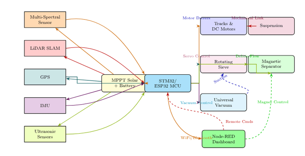
At the core of the robot’s architecture is a hierarchical control system integrating multiple sensing, actuation, and computation subsystems. The robot is powered by a Maximum Power Point Tracking (MPPT) solar array with battery storage, providing energy to a suite of sensors (multi-spectral, LiDAR, GPS, IMU, ultrasonic) and actuators (caterpillar tracks, adaptive suspension, rotating sieve, vacuum, magnetic separator). The central microcontroller (STM32/ESP32) acts as the supervisory controller, executing sensor fusion, motion planning, and actuator coordination.

Figure 1 illustrates the robot control system structure showing the current flow.
The overall system can be mathematically represented in the standard state-space form:
(1) ![\[\dot{X}(t) = A X(t) + B U(t)\]](https://nhsjs.com/wp-content/ql-cache/quicklatex.com-370ce3cc2493b99e5eeb6a581a0d96b6_l3.png "Rendered by QuickLaTeX.com")
(2) ![\[Y(t) = C X(t) + D U(t)\]](https://nhsjs.com/wp-content/ql-cache/quicklatex.com-09e121fbc02ab85b349bc74a29872af3_l3.png "Rendered by QuickLaTeX.com")
where  is the state vector encompassing battery state-of-charge, robot kinematics, sensor states, and actuator positions;
 is the input vector including remote commands, environmental disturbances, and actuator setpoints; and
 is the output vector representing measurable quantities such as robot position, debris detection, and system status.
The  matrix encodes the internal dynamics of each subsystem and their interactions, while
  maps control inputs to state changes. For example, the motion subsystem is governed by:
(3) ![\[\dot{x}_{13} = -d x_{13} + e u_{\text{motor}}\]](https://nhsjs.com/wp-content/ql-cache/quicklatex.com-b5139448019514a90fad3891d97e94a4_l3.png "Rendered by QuickLaTeX.com")
where  is the track velocity and
  is the motor control input. The robot’s position, derived from sensor fusion (LiDAR/GPS/IMU), evolves as:
(4) ![\[\dot{x}_4 = x_{13} \cos(x_8), \quad \dot{x}_5 = x_{13} \sin(x_8)\]](https://nhsjs.com/wp-content/ql-cache/quicklatex.com-35fd86fe244311d58f6bbcb19683f2d3_l3.png "Rendered by QuickLaTeX.com")
with  representing orientation.

Hierarchical Control System Architecture
To clarify organization of the hierarchical control system referenced in the introduction, we present Figure 3, which illustrates interaction between the STM32/ESP32 microcontrollers, sensing modules, actuation subsystems, and the IoT dashboard.

Literature Review
1. In Comprehensive Review of Solar Remote Operated Beach Cleaning Robot by A. Kumar, P. Sharma, and R. Singh, the authors construct a beach-cleaning robot with optimal utilities suited for efficiency and independence, such as solar panels, lithium-ion battery, conceptual description of a camera utilized for navigation, and a conveyor belt system1. Our theoretical design aims to achieve the same task as this design, but our conceptual design of a vacuum-filtration system boasts an ideally more efficient path for debris to be collected, due to an increased force by the vacuum. In addition, our theoretical application of LiDAR working alongside a machine learning assisted camera creates a heightened awareness of navigation by concept.
2. In Remote Controlled Road Cleaning Vehicle by R. Patel and S. Desaithe, the authors provide a hardware component list essential for a remote controlled road cleaning vehicle2. Specific components listed are a DC power supply (similar to our proposal of a lithium-ion battery usage), microcontroller for essential machine interface and control, and a brush mechanism for collecting trash. Our paper proposes a robot design that proposes a conceptual design of a vacuum-filtration system, which boasts an ideally more efficient path for debris to be collected, due to an increased force by the vacuum compared to the brush mechanism. In addition, our theoretical application of LiDAR working alongside a machine learning assisted camera creates the possibility for operating and navigating with independence, instead of using remote control.
3. In Autonomous Robotic Street Sweeping: Initial Attempt for Curbside Sweeping by M. Bergerman and S. Singh, the authors provide an analysis of an engineered autonomous street sweeping robot, utilizing an IMU & GPS autonomous navigation along with a fisheye dual-camera setup to target trash according to the image renders3. Our design offers similar utilizations, but instead of an IMU & GPS system, we utilize a perimeter rendering LiDAR system along with an AEGIS machine-learning assisted camera to accurately differentiate obstacles and trash by concept. Our setting of automation involves an ocean shore, which holds more environmental obstacles than this experiment’s flat, curbside setting, requiring the specific technology in this study to automate these obstacles.
4. In Cleaning Robots in Public Spaces: A Survey and Proposal for Benchmarking Based on Stakeholders Interviews by A. Papadopoulos and L. Marconi, the authors provide an analysis of a combination of interviews of automated robot utilization in public spaces, specifying their performance, capabilities, and ideal requirements for implementation4. This connects to our justifiable decision of utilizing our Lidar + SLAM system being a necessity towards self navigation and cognition.
5. In Modular Robot Used as a Beach Cleaner by G. Muscato and M. Prestifilippo, the authors demonstrate simulations of camera image processing, avoidance simulation, and a theoretical claw-like trash collecting mechanism within a similar ocean shore cleaning robot5. However, our proposal of a theoretical vacuum filtration system considers the possible increase in efficiency of waste collection compared to this paper’s claw design.
6. In OATCR: Outdoor Autonomous Trash-Collecting Robot Design Using YOLOv4-Tiny by H. Chen, L and Zhang, J, the authors propose an outdoor autonomous trash-cleaning robot design, with details of control system structure, robot structure, visual waste detection analysis with mathematical interpretations along with simulations using TACO (Trash annotations in context) assist6. This paper displays an application using a machine learning database to identify trash in a robot’s surroundings, which is a similar approach to our utilization of AEGIS camera waste identification.
7. In Waste Management by a Robot: A Smart and Autonomous Technique by R. Gupta and N. Sharma, the author provides a control system structure for a remote controlled road cleaning vehicle, and even a prototype physical design of the robot7. Specific components listed are microcontrollers (arduino) for essential machine interface and control, and a combination of motor drivers and servo motors for a robotic arm for dynamic trash collection. Our robot design implements a variety of innovations expanding on this foundation. The primary focus of unique innovation is the design of a vacuum-filtration system, which boasts an ideally more efficient path for debris to be collected, due to an increased force by the vacuum. In addition, our theoretical application of LiDAR working alongside a machine learning assisted camera creates the possibility for operating and navigating with independence, instead of using remote control.
8. In Beach Sand Rover: Autonomous Wireless Beach Cleaning Rover by S. Iyer and A. Nair, the authors provide a component list, experimental proposal of infrared sensors combined with a GPS system for independent navigation, and physical models for a claw utilizing road cleaning vehicle8. Our robot design implements a variety of innovations expanding on this foundation. The primary focus of unique innovation is the design of a vacuum-filtration system, which boasts an ideally more efficient path for debris to be collected, due to an increased force by the vacuum. In addition, our theoretical application of LiDAR working alongside a machine learning assisted camera creates possibility for operating and navigating with a heightened independence for avoiding obstacles than GPS + infrared sensors.
9. In Autonomous Trash Collecting Robot by K. Lee and A. Patel, the authors provide a component list, experimental proposal of infrared sensors combined with ultrasonic sensors for surrounding awareness, and physical models for a suction vacuum trash collecting system9. Our robot design implements a variety of innovations expanding on this foundation. The primary focus of unique innovation is the design of a vacuum-filtration system, which boasts an ideally strong and selective accuracy for a variety of debris to be collected, due to the addition of filtration by the vacuum. In addition, our theoretical application of LiDAR working alongside a machine learning assisted camera creates the possibility for operating and navigating with a heightened independence for avoiding obstacles than ultrasonic + infrared sensors.
10. In Autonomous Litter Collecting Robot with Integrated Detection and Sorting Capabilities by A. Rahman and S. Gupta, the authors provide a component list, simulation analysis of infrared sensors combined with ultrasonic sensors for surrounding awareness, along with a camera assisted with TACO (Trash annotations in context) for surrounding trash identification10. Our robot design implements a variety of innovations expanding on this foundation. Our theoretical application of LiDAR working alongside a machine learning assisted camera creates possibility for operating and navigating with a heightened independence for avoiding obstacles compared to the ultrasonic & infrared sensor + camera assisted with TACO, which can only identify trash and cannot identify obstacles like humans in an ocean shore context.
11. In Autonomous Detection and Sorting of Litter Using Deep Learning and Soft Robotic Grippers by P. Proenca and P. Simoes, the authors provide models of a dual fin ray finger design for the waste collecting mechanism along with its architecture, along with object waste detection analysis utilizing a camera assisted with TACO for surrounding trash identification11. Our robot design implements a variety of innovations expanding on this foundation. Firstly, our vacuum filtration design would ensure more force and simultaneous area of intaking, assisted with a filtration of environmental objects in concept. Second, our theoretical application of LiDAR working alongside a machine learning assisted camera creates possibility for operating and navigating with a heightened independence for avoiding obstacles than ultrasonic and infrared sensor + camera assisted with TACO, which can only identify trash and cannot identify obstacles like humans in an ocean shore context.
12. In AI for Green Spaces: Leveraging Autonomous Navigation and Computer Vision for Park Litter Removal by D. Kim and J. Martinez, the authors provide a concise breakdown and analysis of a park litter removal robot12. This design consists of a GPS + Slam under a precise algorithm for autonomous navigation. The design also analyzed 3 different TACO datasets (Trash annotations in context) to determine the most efficient computer vision processing for trash collection. In addition, the final design model displayed utilization of various trash collecting devices, with a conclusion of a rake pickup mechanism giving greatest results. Our robot design implements a variety of innovations expanding on this foundation. Firstly, our vacuum filtration design would ensure more force and simultaneous area of intake, assisted with a filtration of environmental objects in concept. This counters the issue of the analysis of vacuum tested in this paper’s model, where it was too small leading to the inability of collecting big objects, along with a lack of filtration, which gives the ability to selectively avoid collecting environmental objects. Our vacuum system is simulated to be drastically wider with a stronger force. Second, our theoretical application of LiDAR working alongside a machine learning assisted camera creates possibility for operating and navigating with a heightened independence for avoiding obstacles than ultrasonic and infrared sensor + camera assisted with TACO, which can only identify trash and cannot identify obstacles like humans in an ocean shore context.
13. In BeWastMan IHCPS: An Intelligent Hierarchical Cyber-Physical System for Beach Waste Management by M. Rizzo and G. Testa, the authors present BIOBLU as a cyber-physical framework for waste-collecting robots, integrating vision-based litter detection with ML, hierarchical control across robot–edge–cloud layers, GNSS/SLAM-based navigation, modular waste-handling mechanisms, sustainable power solutions, and geotagged data analytics to enable efficient, autonomous, and environmentally sustainable cleanup operations13. Our robot provides an abstract design of a filtration vacuum system, with ability to filter out environmental objects and exceeding size items from mass collectible plastic debris, with a compelling force by context. Our autonomous navigation components are near identical in terms of function.
14. In Design a Beach Cleaning Robot Based on AI and Node-RED Interface for Debris Sorting and Monitor the Parameters by T. Mallikarathne and R. Fernando, the authors provide a beach cleaning robot model with a debris-sifting mechanism, AI model utilizing an identification system of collected debris and a Lidar + GPS model for autonomous navigation14. Our model proposes a similar but an alternate approach to the debris collecting device: a filtration vacuum system, with an ability to filter out environmental objects and exceeding size items from mass collectible plastic debris, with a compelling force by context.
15. In Trash Collection Gadget: A Multi-Purpose Design of Interactive and Smart Trash Collector, by H. Zhou and L. Wang, the authors offer a physical prototype of a robot with a similar task: to portably clean ocean shores of its abundance in plastic debris15. This paper also provides experimental data with trash collection rates varying on displacement. This design boasts a portable conveyor belt system and track-equipped wheels. Our robot design provides a more independent system, with theoretical design of applying components regarding autonomous navigation with equipped awareness, along with a filtration vacuum system for efficient, powerful, and selective debris collection.
16. In Autonomous Beach Cleaning Robot Controlled by Arduino and Raspberry Pi by R. Mehta and A. Khan, the authors provide a component list of a person-operated beach cleaning machine, with a waste collection mechanism consisting of wiper motor, mesh, and a roller pipe16. Our autonomous beach-cleaning robot design is inspired by the mesh applied collector, as while the inspiring paper does not provide specifically detailed reasons for usage, it has inspired the usage of our nets to separate sufficient debris for collection and small and negligible environmental objects such as sand within our vacuum tube collector.
17. In Design and Fabrication of Beach Cleaning Equipment by J. Patil and V. Sharma, the authors provide a detailed component list and a physical model design of an ocean-shore collection mechanism, equipped with a conveyor chain hook arrangement for scooping17. In addition, there has been a 3D CAD model connected along with methodology based on the structure. Our model provides an abstract filtration vacuum mechanism that has the same objective of efficiently collecting waste in its surroundings, but with a greater force and selectivity. While this paper’s design has a standard 4-wheel locomotion system, our locomotive system boasts a caterpillar-track platform for stable movement through the sandy ocean shore. Our robot design also approaches a robot capable of autonomy, but utilizing self-navigation through the utilization of a Lidar system along with a machine-learning assisted camera.
18. In Beach Cleaning Robot by K. Suresh and D. Ramesh, the authors display a beach-cleaning robot component list with a control system structure, along with a 3D render CAD model and a physical prototype for demonstrating the robot structure18. The models have a 4-wheel locomotive system, along with a conveyor belt debris collection mechanism. Our robot design expands on both of these innovations by applying a caterpillar track locomotion system to move through the sandy shore in stability. Our design also provides an abstract filtration vacuum mechanism that has the same objective as the conveyor belt system of efficiently collecting waste in its surroundings, but with a greater force and selectivity.
19. In Design and Development of Beach Cleaning Machine by A. Narayan and R. Kulkarnipaper, the authors provide a system design of an autonomous beach cleaning robot consisting of a component list along with a control system structure19. The paper also provides hardware design overview details towards certain components, and overviews of the motor control system, garbage recognition algorithm, and the communication interface. Our model provides more detailed component breakdowns and of the autonomous processing of a robot applied on an ocean shore, specifically towards an elevated garbage recognition algorithm under more advanced components.
20. In Smart AI-Based Waste Management in Stations by J. Lee and Y. Chen, the authors provide methodology and experimentation towards applying SLAM and 2-D LiDAR towards autonomous navigation20. Specifically, this paper targets Correlative Scan Matching (CSM) towards precise measurements in navigation. In addition, the utilization of a variety of loop closure detection methods towards reducing noise sensitivity is displayed, for an extreme navigation accuracy. Our model provides a stack of GPS and LiDAR measurement models to expand on robot navigation, by specifically employing a fusion network based on Extended Kalman Filter (EKF) within a LiDAR SLAM pipeline. Regarding the topic of autonomous navigation, our paper applies the concept of LiDAR and GPS to an ocean-shore setting for the robot, where human and environmental obstacles are abundant, needing frequent awareness by the robot to safely avoid interaction with them.
21. In Sweeping Robot Based on Laser SLAM by X. Zhang and Y. Liu, the authors provide a SLAM simulation towards robot self navigation, utilizing a Gmapping an algorithm based on the Rao-Blackwellized particle filtering, within the Gazebo simulating software towards precise LiDAR mapping and navigation tests21. Our model provides a stack of GPS and LiDAR measurement models to expand on robot navigation, by specifically employing a fusion network based on Extended Kalman Filter (EKF) within a LiDAR SLAM pipeline. Regarding the topic of autonomous navigation, our paper applies the concept of LiDAR and GPS to an ocean-shore setting for the robot, where human and environmental obstacles are abundant, needing frequent awareness by the robot to safely avoid interaction with them.
22. In Design and Experimental Research of an Intelligent Beach Cleaning Robot Based on Visual Recognition by Q. Jiang, X. Wang, and X. Zhang, the authors applied reinforcement learning towards experimenting with Khepera IV’s omniscience sensors to amplify the robot’s obstacle identifying capabilities, increasing its autonomous function22. While this paper uses 8 infrared sensors for its simulation analysis, our model provides a stack of GPS and infrared LiDAR measurement models to expand on robot navigation, by specifically employing a fusion network based on Extended Kalman Filter (EKF) within a LiDAR SLAM pipeline. Regarding the topic of autonomous navigation, our paper also applies this objective to an ocean-shore setting for the robot, where human and environmental obstacles are abundant, needing frequent awareness by the robot to safely avoid interaction with them. Our simulations regarding additional variables, such as a Machine-learning assisted camera for easier obstacle identification, has been considered for our python simulations.
23. In Diseño e Implementación de un Prototipo de Robot para la Limpieza de Playas by F. Martínez and D. Sánchez, the authors propose a sustainable beach-cleaning robot design, specifically towards its utilization of a rake sand-sifting mechanism towards collecting debris23. This paper also provides a motion torque analysis. Our robot design implements a vacuum filtration design expanding on this foundation. This mechanism would ensure more force and simultaneous area of intake, assisted with a filtration of environmental objects in concept. Our vacuum system is simulated to be drastically wider with a stronger force.
24. In Design and Implement of Beach Cleaning Robot by M. Rahman, T. Hasan, and S. Akterpaper, the authors propose a beach cleaning robot design with a conveyor belt debris collection mechanism, along with a breakdown of the electrical flow control system architecture satisfying the robot operations24. Our robot design implements a vacuum filtration design expanding on this foundation. This mechanism would ensure more force and simultaneous area of intake, assisted with a filtration of environmental objects in concept. Our vacuum system is simulated to be drastically wider with a stronger force. 25. In EcoBot: An Autonomous Beach-Cleaning Robot for Environmental Sustainability Applications by F. M. Talaat, A. Morshedy, M. Khaled, and M. Salem, the authors present the design and implementation of EcoBot, an autonomous beach-cleaning robot utilizing a mechanical arm debris collection system, and YOLO (You Only Look Once) computer vision for easy debris identification in its surroundings, helping navigation25. The robot also utilizes a variety of sensors, including ultrasonic sensors for a more assisted, autonomous navigation. This paper provides a control system architecture, waste detection analytics, and hardware design models of the robot. Our robot design implements a variety of innovations expanding on this foundation. Firstly, our vacuum filtration design would ensure more force and simultaneous area of debris intake, assisted with a filtration of environmental objects in concept. Our vacuum system is conceptualized towards higher efficiency compared to the mechanical arm debris collection system. Second, our theoretical application of LiDAR working alongside a machine learning assisted camera creates possibility for operating and navigating with a heightened independence for avoiding obstacles, which is a similar alternate approach compared to EcoBot’s YOLO application and ultrasonic sensor system for autonomous navigation.
Detailed Description of the Robot Control System
The system is modular and consists of a sequence of computational and physical blocks that transform the high-level path planning strategy into executable control commands. Each block is explained below.
Vector Field Generator
This module constructs a vector field across the robot’s environment by summing attractive and repulsive forces. The attractive force is directed toward the goal, while the repulsive forces are perpendicular to the attractive vector and modulated by a Gaussian function. The resultant vector  at each position is given by:
![\[\vec{V}_p = \vec{V}_T + \sum_{i=1}^{n} \vec{V}_{T90_i}\]](https://nhsjs.com/wp-content/ql-cache/quicklatex.com-f42deac227c8340127893d82e37762c4_l3.png "Rendered by QuickLaTeX.com")
where  is the target-directed attractive force and
  represents the orthogonal repulsive force due to the
  -th obstacle. The output of this block is a direction of motion
  , defined as:
![\[\theta_{in}(t) = \angle \vec{V}_p\]](https://nhsjs.com/wp-content/ql-cache/quicklatex.com-e550e3a0b44401eb79b7d5088614cbb0_l3.png "Rendered by QuickLaTeX.com")
Clarification: Vector Field Generator for Navigation
The Vector Field Generator computes a navigation direction at every position on the map by combining:
- Attractive force towards the goal, guiding the robot’s motion.
- Repulsive forces from obstacles, discouraging movement close to them.
Let  denote the robot’s current position and
  the goal.
Attractive Vector
The normalized attractive vector points directly from the robot to the goal:
![\[\vec{V}_T = \frac{p_{goal} - p_{robot}}{\left|\left| p_{goal} - p_{robot} \right|\right|}\]](https://nhsjs.com/wp-content/ql-cache/quicklatex.com-6f08d1d44eef8390f0d21eed7225dfab_l3.png "Rendered by QuickLaTeX.com")
This defines the main direction of travel.
Repulsive Vectors
For each obstacle at position  :
:
- Compute the vector from robot to obstacle:

- Rotate
 by
by  (counterclockwise) to get a unit vector
  perpendicular to the attractive direction.
 - The magnitude of the repulsive effect is determined by a Gaussian envelope:
![\[w_i = \rho_i \exp \left( - \frac{ \left|\left| p_\text{robot} - p_{\text{obs},i} \right|\right|^2 }{ 2 \sigma^2 } \right)\]](https://nhsjs.com/wp-content/ql-cache/quicklatex.com-68f460ad88fb70965d9e141e66b944b4_l3.png "Rendered by QuickLaTeX.com")
- where
 controls repulsion strength, and
  sets the distance scale.
 - The total repulsive force is then
 .
.
Combined Navigation Vector
The final direction is given by:
![\[\vec{V}_p = \vec{V}_\mathrm{T} + \sum_i w_i \vec{V}_{\mathrm{T},90i}\]](https://nhsjs.com/wp-content/ql-cache/quicklatex.com-3a5292493826f83333a16e664155e079_l3.png "Rendered by QuickLaTeX.com")
The robot follows the angle of , which smoothly guides it towards the goal while veering away from obstacles, but always with a component directed to the goal.
Illustrative Diagram
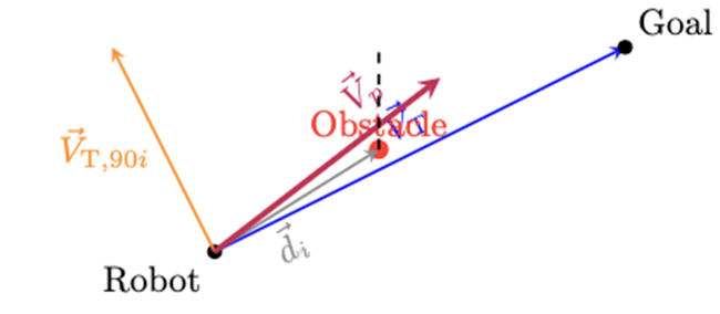 ). The orange arrow is the repulsive (perpendicular) component, modulated in strength by Gaussian proximity to the obstacle (red). The purple arrow is the final direction which ultimately steers the robot clear of the obstacle while keeping it headed for the goal.
This construction achieves smooth, goal-directed navigation that can safely skirt obstacles without producing the oscillatory “zig-zag” or deadlocks seen in other potential field methods, as repulsive influences only serve to laterally nudge the heading, never to fully reverse it.
Fourier Transform Block
To ensure that the robot is capable of physically executing the desired trajectory, the heading signal is analyzed in the frequency domain using a Fourier Transform:
![\[\Theta_{in}(j\omega) = \mathcal{F}\left\{ \theta_{in}(t) \right\}\]](https://nhsjs.com/wp-content/ql-cache/quicklatex.com-2aa13c41d0f0c22abaa635e8d8ab38e9_l3.png "Rendered by QuickLaTeX.com")
This frequency representation is compared against the known bandwidth of the robot’s actuators. If the frequency content of the signal exceeds this bandwidth, the robot’s speed must be reduced to avoid overshooting or oscillation.
Robot Simulator
This block virtually simulates the robot’s response to the vector field before actual execution. It stores the heading command and evaluates if the robot can track the path with minimal error. This predictive module prevents infeasible commands from being sent to the physical robot.
Controller
The controller compares the stored heading with the robot’s actual orientation to compute angular velocity  . Additionally, the forward velocity
  is calculated using the centripetal acceleration constraint:
![\[V_{in}' = \frac{a_{\text{const}}}{\omega_{in}}\]](https://nhsjs.com/wp-content/ql-cache/quicklatex.com-3bf25cfbbfb03f8367d1b9db513dd600_l3.png "Rendered by QuickLaTeX.com")
The computed forward and angular velocities are then transformed into left and right wheel velocities using the transformation:
![\[\begin{bmatrix}V_{in}^L \\V_{in}^R\end{bmatrix}=\begin{bmatrix}1 & -L/2 \\1 & L/2\end{bmatrix}\begin{bmatrix}V_{in}' \\\omega_{in}\end{bmatrix}\]](https://nhsjs.com/wp-content/ql-cache/quicklatex.com-6822d116bed180adf54a140c81d05f78_l3.png "Rendered by QuickLaTeX.com")
where  is the wheelbase of the robot.
Robot
The robot executes the commands  by driving its left and right wheels at the corresponding velocities
  . The robot’s trajectory is continuously corrected based on the heading and velocity feedback from the controller.
Robot Plant Model 
This block models the dynamic behavior of the robot’s velocity response. In simulation, a first-order linear system with time delay is used:
![\[G(s) = \frac{K_V e^{-T_D s}}{1 + T_1 s}\]](https://nhsjs.com/wp-content/ql-cache/quicklatex.com-a453b0bc9e24e45afc7476c4ac8e3a56_l3.png "Rendered by QuickLaTeX.com")
where  is a gain factor,
  is the system time constant, and
  is the communication/processing delay. The model is calibrated using step-response experiments and used in simulation to ensure accurate trajectory prediction.
The integration of these blocks ensures the robot navigates complex environments safely and efficiently, while dynamically adapting to its physical constraints.
The modular state-space model enables the systematic design of feedback controllers for each subsystem, as well as the analysis of system stability, controllability, and observability. The IoT dashboard provides a human-in-the-loop supervisory layer, allowing for remote monitoring and command injection.
This control-centric modeling framework supports the implementation of advanced control strategies (e.g., optimal, adaptive, or robust control) and facilitates future extensions, such as multi-robot coordination or learning-based adaptation, within a principled systems engineering context.
Robot Perception-Decision-Action Workflow
A robust perception-decision-action pipeline is central to the autonomous operation of the beach-cleaning robot. The full control architecture, from environmental sensing to mechanical actuation, can be summarized as follows:
Workflow description:
- Sensors: The robot continuously acquires data on terrain, obstacles, debris, and its internal state using its sensor suite.
- Sensor Fusion and Preprocessing: Raw sensor data are fused and filtered to produce robust, high-confidence environment state estimates (e.g., position, nearby obstacles, detected debris).
- Controller/Decision Logic: This module receives the estimated state, plans a motion/path, and generates actuator commands based on integrated models (e.g., vector-field navigation, feedback control, sorting logic).
- Actuators: Commands are transmitted to all robot effectors (tracks, suspension, vacuum/sieve, separator), interacting with the environment.
- Feedback Loop: The results of the actions update the sensory input, closing the loop for continuous, adaptive operation.
This pipeline ensures that the robot autonomously closes the loop between perception, control, and actuation in a robust and extensible fashion. The workflow has been illustrated in Figure 4.

Integration of Multi-Spectral Camera with AEGIS Machine Learning in Control System
The beach-cleaning robot utilizes an advanced multi-spectral camera system equipped with the AEGIS machine learning (ML) application to achieve precise debris identification. This integration plays a critical role in the robot’s perception and control architecture.
State-Space Representation
In the modular state-space modeling framework, the multi-spectral camera sensor output, enhanced via AEGIS ML-based debris classification, is represented as a key sensor state variable denoted by  . This state captures the processed debris detection signal within the robot’s environment.
Mathematically, the sensor dynamics can be modeled by a first-order linear system with external environmental debris input  :
:
![\[\dot{x}_3 = -f x_3 + g u_3,\]](https://nhsjs.com/wp-content/ql-cache/quicklatex.com-23d8fca315364644f6d22f20a2297f3e_l3.png "Rendered by QuickLaTeX.com")
where  represents the sensor decay or filtering rate, and
  models the sensor response gain.
Influence on Robot Commands
The debris detection state  directly impacts actuator commands responsible for waste collection. Specifically, the uptake subsystems for vacuum and sieve adjust their actuation based on the debris detection signal, as reflected by the dynamics:
![\[\dot{x}_{15} = -h x_{15} + j \left( u_4 + x_3 \right),\]](https://nhsjs.com/wp-content/ql-cache/quicklatex.com-1f5f7a6eb6b4326caec9a729149d9890_l3.png "Rendered by QuickLaTeX.com")
![\[\dot{x}_{16} = -k x_{16} + l u_4,\]](https://nhsjs.com/wp-content/ql-cache/quicklatex.com-e5155e5a31135755c9b650dcc30177b5_l3.png "Rendered by QuickLaTeX.com")
where  and
and  represent the sieve speed and vacuum pressure states, respectively, and
  is the actuator setpoint command.
Here, the inclusion of in the input to the sieve speed dynamics indicates that increased debris detection results in intensified sieve operation. Thus, the ML-driven sensor state dynamically modulates waste collection mechanisms.
Control Architecture Implications
While the debris detection signal is part of the overall state vector  , the ML component also interfaces with higher-level decision modules within the STM32/ESP32 microcontroller. The system leverages AEGIS’s classification outputs to:
- Differentiate between environmentally harmful debris and benign objects,
- Selectively activate actuators for targeted waste collection,
- Prioritize navigation paths toward debris-congested areas,
- Reduce false-positive activations through adaptive machine learning inference.
This perception-driven feedback creates an adaptive control loop where sensor-derived knowledge informs and adjusts robot actions in real time.
The integration of the multi-spectral camera and AEGIS ML technology is formally encapsulated as a measurable state in the robot’s state-space model. Its influence cascades through the control hierarchy, enhancing vacuum and sieve actuation and enabling perception-informed autonomous behavior.
This design approach ensures robust, selective, and efficient debris cleanup by coupling advanced sensing and machine learning tightly with control system dynamics.
Construction of the Global State Space Model
The state-space representation introduced earlier has the compact form
![\[\dot{X}(t) = A X(t) + B U(t),\]](https://nhsjs.com/wp-content/ql-cache/quicklatex.com-4d533c569d6a609ec78380e1343acb5e_l3.png "Rendered by QuickLaTeX.com")
but the process by which subsystem dynamics are combined into the global matrices and was not previously detailed. We provide that explanation here.
Subsystem Equations
Each physical subsystem—battery, locomotion, suspension, vacuum/sieve, sensors—is first described by a local state equation of the form
![\[\dot{x}_i(t) = A_i x_i(t) + B_i u_i(t),\]](https://nhsjs.com/wp-content/ql-cache/quicklatex.com-884cec35c65d3a5c8a13bbf4752f9937_l3.png "Rendered by QuickLaTeX.com")
where  are subsystem states,
  are local inputs, and
  ,
,  are subsystem dynamics matrices. For example:
- Battery model:
 [state-of-charge, bus voltage],
 - Motion model:
 [position, heading, track velocity],
 - Suspension:
 ,
, - Vacuum/sieve:
 ,
, - Environmental load: (disturbance), etc.
Stacking Procedure
The global state vector is formed by concatenation:
![\[X(t) = \begin{bmatrix}x_1^\top & x_2^\top & \cdots & x_k^\top\end{bmatrix}^\top,\]](https://nhsjs.com/wp-content/ql-cache/quicklatex.com-902e74c4b47b174bbe5069778dbcc794_l3.png "Rendered by QuickLaTeX.com")
with dimension  . Similarly, the global input vector is
![\[U(t) = \begin{bmatrix}u_1^\top & u_2^\top & \cdots & u_k^\top\end{bmatrix}^\top,\]](https://nhsjs.com/wp-content/ql-cache/quicklatex.com-2d77e4d2e86f307f84c0d489e8e5e2b4_l3.png "Rendered by QuickLaTeX.com")
with dimension  .
.
If subsystems are completely decoupled, the global matrices take block-diagonal form:
![\[A = \begin{bmatrix}A_1 & 0 & \cdots & 0 \\0 & A_2 & \cdots & 0 \\\vdots & \vdots & \ddots & \vdots \\0 & 0 & \cdots & A_k\end{bmatrix}, \qquadB = \begin{bmatrix}B_1 & 0 & \cdots & 0 \\0 & B_2 & \cdots & 0 \\\vdots & \vdots & \ddots & \vdots \\0 & 0 & \cdots & B_k\end{bmatrix}.\]](https://nhsjs.com/wp-content/ql-cache/quicklatex.com-92f8d63b126ef43192599bef01b1dbed_l3.png "Rendered by QuickLaTeX.com")
In practice, beach operation introduces couplings between subsystems (e.g., suspension deformation affects locomotion drag; vacuum load affects battery dynamics). These appear as
off-diagonal blocks in and . For instance, the coupling between track velocity and suspension is encoded as a nonzero off-diagonal entry  .
.
Visual Schematic
The stacking can be visualized as shown in Figure 5, where local subsystem dynamics are assembled into the global model:

In short, the complete state-space model is obtained by stacking all subsystem equations in block form and explicitly adding off-diagonal terms for physical couplings. This method makes the structure of and transparent, and provides a modular pathway to update the global dynamics whenever subsystems are refined or re-identified.
Consistent State-Space Model Definitions and Simplified Analysis
The core dynamics of the beach-cleaning robot are captured within a state-space modeling framework. To avoid ambiguity, we provide explicit definitions for each symbol and simplify the presentation to reflect the actual implementation.
State-Space Model Structure
The system is modeled (possibly with both linear and nonlinear terms) as
(5) ![\[\dot{x}(t) = A x(t) + B u(t) + f(x,t) \]](https://nhsjs.com/wp-content/ql-cache/quicklatex.com-d18f8c3bf854ba97b5c8ba612956ec4a_l3.png "Rendered by QuickLaTeX.com")
(6) ![\[y(t) &= C x(t) + D u(t) \]](https://nhsjs.com/wp-content/ql-cache/quicklatex.com-da919844f54dd11e6f0bb070a298257e_l3.png "Rendered by QuickLaTeX.com")
Where:
 is the state vector (with all main subsystem states)
 is the input vector (external controls, setpoints)
 is the output vector (sensor or monitored outputs)
 are system matrices of appropriate dimension
 represents potentially nonlinear coupling (e.g., position kinematics)
Explicit State and Input Definitions
For the implemented and simulated model, the principal states are:
![\[x(t) =\begin{bmatrix}x_1 \\x_2 \\x_3 \\x_4 \\x_5 \\x_8 \\x_{13} \\x_{15} \\x_{16}\end{bmatrix}=\begin{bmatrix}\text{Battery SoC} \\\text{Bus voltage (V)} \\\text{Debris detection signal} \\\text{Position } x \text{ (m)} \\\text{Position } y \text{ (m)} \\\text{Orientation } \theta \text{ (rad)} \\\text{Track velocity (m/s)} \\\text{Sieve rotational speed} \\\text{Vacuum subsystem pressure}\end{bmatrix}\]](https://nhsjs.com/wp-content/ql-cache/quicklatex.com-b95d64af0a70f76dad0babfe0aab7067_l3.png "Rendered by QuickLaTeX.com")
The input vector is
![\[u(t) =\begin{bmatrix}u_1 \\u_2 \\u_3 \\u_4\end{bmatrix}=\begin{bmatrix}\text{Remote track command} \\\text{Solar charging input} \\\text{Environmental disturbance (debris)} \\\text{Actuator setpoint (vacuum/sieve)}\end{bmatrix}\]](https://nhsjs.com/wp-content/ql-cache/quicklatex.com-701224151f06783f8b35726d4dc39ebe_l3.png "Rendered by QuickLaTeX.com")
Subsystem Dynamics
The system is block modular. The major subsystems are:
Power Subsystem:
(7) ![\[\dot{x}_1 &= -\frac{1}{C_\text{batt}} i_\text{load} + \frac{1}{C_\text{batt}} u_2 \]](https://nhsjs.com/wp-content/ql-cache/quicklatex.com-9f2e9f28bfcaf8dc8f439712e1930e61_l3.png "Rendered by QuickLaTeX.com")
(8) ![\[\dot{x}_2 &= -\alpha x_2 + \beta u_2 - \gamma i_\text{load} \]](https://nhsjs.com/wp-content/ql-cache/quicklatex.com-bcc0edc1615cf7d85ebb3b44b9462c3e_l3.png "Rendered by QuickLaTeX.com")
with  SoC,
SoC,  bus voltage,
  a function of actuators.
Debris Sensor Filter:
(9) ![\[\dot{x}_3 = -f x_3 + u_3 \]](https://nhsjs.com/wp-content/ql-cache/quicklatex.com-02bd3b4c8dd0696e0a32259c7a47d4ce_l3.png "Rendered by QuickLaTeX.com")
with  the debris/environment disturbance input.
Tracks (locomotion):
(10) ![\[\dot{x}_{13} = -d x_{13} + e \, u_\mathrm{motor} \]](https://nhsjs.com/wp-content/ql-cache/quicklatex.com-6d587ba2e2cc3ade2d8889dc21210c18_l3.png "Rendered by QuickLaTeX.com")
where  is a (potentially feedback-controlled) motor command.
Position/heading (kinematics):
(11) ![\[\dot{x}_4 &= x_{13} \cos(x_8) \]](https://nhsjs.com/wp-content/ql-cache/quicklatex.com-2cd69d0acfcad547a3b55cf15a7cc729_l3.png "Rendered by QuickLaTeX.com")
(12) ![\[\dot{x}_5 &= x_{13} \sin(x_8) \]](https://nhsjs.com/wp-content/ql-cache/quicklatex.com-6c0b00176b1a9d1109b831dc90b4c61a_l3.png "Rendered by QuickLaTeX.com")
(13) ![\[\dot{x}_8 &= \text{(steering command)} \]](https://nhsjs.com/wp-content/ql-cache/quicklatex.com-5d6e773cf735385cfeca3cdca37ddc06_l3.png "Rendered by QuickLaTeX.com")
Vacuum and sieve:
(14) ![\[\dot{x}_{15} &= -h x_{15} + j (u_4 + x_3) \]](https://nhsjs.com/wp-content/ql-cache/quicklatex.com-4ac170126680c241787483ff06afd893_l3.png "Rendered by QuickLaTeX.com")
(15) ![\[\dot{x}_{16} &= -k x_{16} + l u_4 \]](https://nhsjs.com/wp-content/ql-cache/quicklatex.com-955d0650753f04f1498be86f3e98f6b3_l3.png "Rendered by QuickLaTeX.com")
Summary Table of Variables
| Symbol | Meaning | Python Variable |
|---|---|---|
| x1 | Battery SoC (state-of-charge) | x1 |
| x2 | Bus voltage | x2 |
| x3 | Debris sensor signal | x3 |
| x4 | x-position | x4 |
| x5 | y-position | x5 |
| x8 | Orientation (heading, radians) | x8 |
| x13 | Track velocity | x13 |
| x15 | Sieve speed | x15 |
| x16 | Vacuum pressure | x16 |
| u1 | Remote (track) command | u1 |
| u2 | Solar charger input | u2 |
| u3 | Debris/environment disturbance | u3 |
| u4 | Vacuum/sieve actuator setpoint | u4 |
This notation therefore covers all equations used in the theoretical section and in the practical simulation framework, ensuring clarity, reproducibility, and ease of extension for further development.
Simulation Implementation and Role in Design
A comprehensive simulation framework was developed and implemented for the autonomous beach-cleaning robot to verify theoretical models, validate subsystem interactions, and inform overall design choices.
Implementation and Code Structure
The simulator, written in Python, includes explicit code for each major subsystem and their interconnections. Key components and modeling approaches are:
- Power Subsystem: Modeled with differential equations for battery state-of-charge (
 ) and bus voltage (
 ):
):
![\[\dot{x}_1 &= -\frac{1}{C}i_{\text{load}} + \frac{1}{C}i_{\text{solar}} \]](https://nhsjs.com/wp-content/ql-cache/quicklatex.com-e18ff6510079127db969021d14f70f7e_l3.png "Rendered by QuickLaTeX.com")
![\[\dot{x}_2 &= -\alpha x_2 + \beta i_{\text{solar}} - \gamma i_{\text{load}}\]](https://nhsjs.com/wp-content/ql-cache/quicklatex.com-835b987c5480e5b385275d20b278b844_l3.png "Rendered by QuickLaTeX.com")
- Motion Subsystem: The velocity of the robot’s tracks, , is governed by
![\[\dot{x}_{13} = -d x_{13} + e\, u_{\text{motor}}\]](https://nhsjs.com/wp-content/ql-cache/quicklatex.com-4e0a84330cc1d2bb8e2b37c7be8ddc1e_l3.png "Rendered by QuickLaTeX.com")
- Debris Detection Subsystem:
![\[\dot{x}_3 = -f x_3 + g\, u_3\]](https://nhsjs.com/wp-content/ql-cache/quicklatex.com-12173b79e06823b0a8f5f34fcc4d8094_l3.png "Rendered by QuickLaTeX.com")
- Position Kinematics and Navigation:
![\[\dot{x}_4 &= x_{13} \cos(x_8) \]](https://nhsjs.com/wp-content/ql-cache/quicklatex.com-75450565710ef45bbab0746839b7ebcc_l3.png "Rendered by QuickLaTeX.com")
![\[\dot{x}_5 &= x_{13} \sin(x_8) \]](https://nhsjs.com/wp-content/ql-cache/quicklatex.com-09a06e5ad29c0f1c5ce66e568092a385_l3.png "Rendered by QuickLaTeX.com")
![\[\dot{x}_8 &= \omega\]](https://nhsjs.com/wp-content/ql-cache/quicklatex.com-e9afbe139b3214aab553a2d9d43daa63_l3.png "Rendered by QuickLaTeX.com")
- Vacuum and Sieve Subsystems:
![\[\dot{x}_{15} &= -h x_{15} + j(u_4 + x_3) \]](https://nhsjs.com/wp-content/ql-cache/quicklatex.com-0e0834a2ea85c8a547017523b76398c6_l3.png "Rendered by QuickLaTeX.com")
![\[\dot{x}_{16} &= -k x_{16} + l u_4\]](https://nhsjs.com/wp-content/ql-cache/quicklatex.com-e856dd5fbca8e6a0c0547ccb9287d659_l3.png "Rendered by QuickLaTeX.com")
- Integrated System: All equations are stacked forming the system dynamics
![\[\dot{X}(t) = f(X(t), U(t))\]](https://nhsjs.com/wp-content/ql-cache/quicklatex.com-c84855b153250edd20fd22f1dc0ed4db_l3.png "Rendered by QuickLaTeX.com")
where aggregates all subsystem states and  is the input vector.
The code utilizes Numpy, scipy.integrate.solve_ivp for integration, and matplotlib for plotting simulation results.
Use of Simulation Outputs in Robot Design
- Subsystem Validation: Each modeled subsystem behaved as predicted, confirming stability (e.g., under Lyapunov analysis) and controllability.
- Integrated Behavior: Simulations produced trajectories for robot position, SoC (State of Charge), and actuator/sensor states, helping validate that control strategies and couplings work as intended.
- Design Decisions Guided by Simulation:
– Verified that hardware and control constraints (such as actuator bandwidth) were respected through frequency-domain analysis (e.g., Fourier transforms).
– Confirmed that system outputs, such as tracking performance and robustness, met specification through RMS error analysis and Monte Carlo robustness tests.
– Supported selection and tuning of controller parameters for safe, efficient, and reliable operation under expected environmental disturbances.
- Reported Results: Figures throughout the paper are direct outputs from the simulation, demonstrating transient responses, SoC and voltage stability, trajectory tracking, and subsystem interplay.
Frequency-Based Speed Adjustment Algorithm
To ensure accurate trajectory tracking without exceeding actuator physical limitations, the robot’s heading command  is processed through a frequency-domain analysis. This approach guarantees the actuator bandwidth constraints are respected, preventing overshoot and oscillatory behavior.
Frequency Content Analysis
The desired heading signal is converted to the frequency domain via the Fourier Transform:
![\[\Theta_{\text{in}}(j\omega) = \mathcal{F}\left\{\theta_{\text{in}}(t)\right\}.\]](https://nhsjs.com/wp-content/ql-cache/quicklatex.com-0101f7deb0495a445bca847920327e9f_l3.png "Rendered by QuickLaTeX.com")
The magnitude spectrum  is inspected to identify the bandwidth characteristics of the command.
Actuator Bandwidth Constraint
Let  denote the known cutoff frequency of the robot’s actuators, determined from actuator specifications and empirical testing. The actuator is assumed capable of faithfully tracking input signals with frequency components below , while higher frequencies induce errors or mechanical strain.
Speed Reduction Algorithm
The algorithm to adjust the robot’s speed based on the heading signal’s frequency content is as follows:
1. Compute the power spectral density (PSD) of from  .
.
2. Define the high-frequency energy as
![\[E_{\text{high}} = \int_{\omega_c}^{\infty} |\Theta_{\text{in}}(j\omega)|^2 \, d\omega.\]](https://nhsjs.com/wp-content/ql-cache/quicklatex.com-a82a95e1fb059cfa76440e4d15e363f9_l3.png "Rendered by QuickLaTeX.com")
3. Define the total energy as
![\[E_{\text{total}} = \int_0^{\infty} |\Theta_{\text{in}}(j\omega)|^2 \, d\omega.\]](https://nhsjs.com/wp-content/ql-cache/quicklatex.com-debacafa0542a0f2879391576af7b056_l3.png "Rendered by QuickLaTeX.com")
4. Calculate the ratio
![\[r = \frac{E_{\text{high}}}{E_{\text{total}}}.\]](https://nhsjs.com/wp-content/ql-cache/quicklatex.com-99878a3b9174df6350cc0a14b7d3ed04_l3.png "Rendered by QuickLaTeX.com")
5. If  exceeds a threshold
  (e.g.,
  ), indicating significant high-frequency content, reduce the forward speed
  proportionally according to:
![\[V^\prime_{\text{in,new}} = V^\prime_{\text{in,orig}} \times (1 - \kappa r),\]](https://nhsjs.com/wp-content/ql-cache/quicklatex.com-192bf44389a48e0db9e6575d1703c7da_l3.png "Rendered by QuickLaTeX.com")
where  is a tuning parameter (
 ) controlling the sensitivity of speed reduction.
6. Recalculate the heading signal corresponding to the new reduced speed and repeat the frequency analysis until  .
.
This iterative speed scaling ensures that the command trajectory remains within actuator capabilities by smoothing out rapid heading changes that exceed physical limits.
Rationale and Literature Context
The approach is consistent with established control strategies where:
- High-frequency reference components cause actuator saturation or tracking errors, compromising system stability.
- Smoothing the input signal by reducing command speeds limits bandwidth demand to actuator feasible range.
- The thresholding parameter and reduction factor can be tuned based on empirical actuator response and robustness margins.
In effect, this frequency-domain speed adjustment functions as a bandwidth-aware trajectory scaling method, foundational to the robot’s control framework. By rigorously linking heading signal spectral content to speed commands, the system prevents actuator saturation and promotes robust, precise beach-cleaning operations.
Control Systems Structure and Background
Overall State Space Model for Beach Cleaning Robot
Identifying Subsystems and States
From the overall system diagram, the major subsystems and their representative state variables can be listed as follows:
| Subsystem | Example State Variables |
|---|---|
| MPPT Solar + Battery | Battery SoC (x1), Bus voltage (x2) |
| Multi-Spectral Sensor (AEGIS) | Last detected debris type (x3) |
| LiDAR SLAM (Luminar IRIS) | Robot position/heading (x4, x5) |
| GPS | Robot position (x6, x7) |
| IMU | Orientation, angular rates (x8, x9, x10) |
| Ultrasonic Sensors | Obstacle distances (x11) |
| STM32/ESP32 Microcontroller | Internal controller states (x12, …) |
| Caterpillar Tracks + DC Motors | Track velocities (x13) |
| Adaptive Suspension | Suspension positions (x14) |
| Rotating Cylindrical Sieve | Sieve angle/speed (x15) |
| Universal Vacuum + Mini Vacuums | Vacuum pressure (x16) |
| Magnetic Separator | Separator state (x17) |
| Node-RED IoT Dashboard | Last command received (x18) |
Input and Output Vectors
Input vector () may include:
![\[U = \begin{bmatrix}u_1 \\ u_2 \\ u_3 \\ u_4 \\ \ldots\end{bmatrix}\]](https://nhsjs.com/wp-content/ql-cache/quicklatex.com-d64a7a071b567ba497d0abc075fa6070_l3.png "Rendered by QuickLaTeX.com")
where, for example:
-
 : Remote commands (from dashboard)
  : Power input (solar charging)
- : Environmental disturbances (e.g., debris, obstacles)
- : Setpoints for actuators (e.g., motor, vacuum, sieve)
Output vector ( ) may include:
- Robot position, orientation, velocity
- Sensor readings (debris type, obstacles)
- Battery SoC, voltage
- Data sent to dashboard
Example State-Space Equations
Let the overall state vector be:
![\[X = \begin{bmatrix}x_1 \\ x_2 \\ x_3 \\ x_4 \\ x_5 \\ x_6 \\ x_7 \\ x_8 \\ x_9 \\ x_{10} \\ x_{11} \\ x_{12} \\ x_{13} \\ x_{14} \\ x_{15} \\ x_{16} \\ x_{17} \\ x_{18}\end{bmatrix}\]](https://nhsjs.com/wp-content/ql-cache/quicklatex.com-9435ea22961b0c23a4613cd15729eb8b_l3.png "Rendered by QuickLaTeX.com")
and the input vector:
The general state-space equations are:
![\[\dot{X} = A X + B U\]](https://nhsjs.com/wp-content/ql-cache/quicklatex.com-2635aac72737b2cc90f2dfa711f34cee_l3.png "Rendered by QuickLaTeX.com")
![\[Y = C X + D U\]](https://nhsjs.com/wp-content/ql-cache/quicklatex.com-817424d59692783aa3970513262f4f6d_l3.png "Rendered by QuickLaTeX.com")
Block Structure of Matrices
Given the modular nature, the and matrices are block matrices:
- : Diagonal blocks model internal dynamics of each subsystem (e.g., battery, motors, sensors).
- Off-diagonal blocks: Model coupling between subsystems (e.g., how vacuum pressure affects debris collection).
- : Maps control inputs to the states they affect (e.g., motor voltage to track velocity).
-
 : Maps states to outputs (e.g., which states are sent to the dashboard).
 -
 : Usually sparse; nonzero only if there is a direct, instantaneous effect of input on output.
Example: Expanded Equations for Key Subsystems
a) Power subsystem
![\[\dot{x}_1 &= -\frac{1}{C} (i_{load}) + \frac{1}{C} (i_{solar}) \]](https://nhsjs.com/wp-content/ql-cache/quicklatex.com-8e36c9ede83e7113ed93bdc4f6c1b481_l3.png "Rendered by QuickLaTeX.com")
![\[\dot{x}_2 &= -a x_2 + b i_{solar} - c i_{load}\]](https://nhsjs.com/wp-content/ql-cache/quicklatex.com-90d3089d69844ee3bb8fe3f9dd07ca5c_l3.png "Rendered by QuickLaTeX.com")
b) Motion subsystem (tracks)
![\[\dot{x}_{13} = -d x_{13} + e u_{motor}\]](https://nhsjs.com/wp-content/ql-cache/quicklatex.com-4323e7ad06198b2910dcb99d87764bcf_l3.png "Rendered by QuickLaTeX.com")
c) Debris detection (sensor)
![\[\dot{x}_3 = -f x_3 + g (\text{debris input})\]](https://nhsjs.com/wp-content/ql-cache/quicklatex.com-dfe42a0f7a055319ee657675c07c84cc_l3.png "Rendered by QuickLaTeX.com")
d) Sieve/vacuum
![\[\dot{x}_{15} &= -h x_{15} + j u_{sieve} \]](https://nhsjs.com/wp-content/ql-cache/quicklatex.com-29e99f28929a3b85e9946ea616704654_l3.png "Rendered by QuickLaTeX.com")
![\[\dot{x}_{16} &= -k x_{16} + l u_{vacuum}\]](https://nhsjs.com/wp-content/ql-cache/quicklatex.com-1c1b612f3d2327de4039d750f1819db0_l3.png "Rendered by QuickLaTeX.com")
e) Robot position (from LiDAR/GPS/IMU fusion)
![\[\dot{x}_5 &= x_{13} \sin(x_8)\]](https://nhsjs.com/wp-content/ql-cache/quicklatex.com-5564679d0fdded0b7f93ae0888f1fb1a_l3.png "Rendered by QuickLaTeX.com")
All these equations can be stacked into the large and matrices.
Full State-Space Model (Symbolic Form)
![\[\begin{bmatrix}\dot{x}_1 \\ \dot{x}_2 \\ \dot{x}_3 \\ \dot{x}_4 \\ \vdots \\ \dot{x}_{17} \\ \dot{x}_{18}\end{bmatrix}=A\begin{bmatrix}x_1 \\ x_2 \\ x_3 \\ x_4 \\ \vdots \\ x_{17} \\ x_{18}\end{bmatrix}+B\begin{bmatrix}u_1 \\ u_2 \\ u_3 \\ \vdots\end{bmatrix}\]](https://nhsjs.com/wp-content/ql-cache/quicklatex.com-0c0a3c2430d16642f2c0aa6e268bc119_l3.png "Rendered by QuickLaTeX.com")
where , , , are constructed by combining the dynamics and interactions of all subsystems.
The following gives the control system structure of the entire robot.
Overall Control System Structure
Nonlinear State-Space Representation
The assumption of a linear time-invariant (LTI) system in modeling the robot dynamics is not fully justifiable for beach environments. Sand deformation, actuator slip, suspension compliance, and debris interactions introduce pronounced nonlinearities that cannot be ignored without compromising model validity. To address this criticism, we reformulate the dynamics using a nonlinear state-space model:
(16) ![\[\dot{X}(t) = f(X(t),U(t),t), \quad Y(t) = h(X(t),U(t),t), \]](https://nhsjs.com/wp-content/ql-cache/quicklatex.com-b00042bdf630e126fcfb39be9958ff91_l3.png "Rendered by QuickLaTeX.com")
where  is the full robot state vector,
  is the input vector,
and  are nonlinear vector fields capturing the coupling between subsystems and the environment.
Example Nonlinear Dynamics For the motion subsystem with track velocity and orientation  , we include nonlinear slip and drag effects:
(17) ![\[\dot{x}_{13} &= -d \, x_{13} + e \, u_{\text{motor}} - \alpha x_{13}^2 \operatorname{sgn}(x_{13}), \]](https://nhsjs.com/wp-content/ql-cache/quicklatex.com-c9225b2fce1ccd93884ad69b56c51d7b_l3.png "Rendered by QuickLaTeX.com")
(18) ![\[\dot{x}_{4} &= x_{13}\cos(x_{8}), \]](https://nhsjs.com/wp-content/ql-cache/quicklatex.com-49658b90e32cb2d0995daab4c19db999_l3.png "Rendered by QuickLaTeX.com")
(19) ![\[\dot{x}_{5} &= x_{13}\sin(x_{8}), \]](https://nhsjs.com/wp-content/ql-cache/quicklatex.com-9dd016cf3738abc6a709413c5c7845b8_l3.png "Rendered by QuickLaTeX.com")
where  models quadratic velocity drag due to granular resistance in sand. Unlike the linear model, this representation reflects how resistance grows nonlinearly with speed.
Suspension–Track Coupling Suspension deformation () interacts with track dynamics:
(20) ![\[\dot{x}_{14} &= f_{1}(x_{14}) + g_{1}(x_{14}) u_{\text{susp}}, \]](https://nhsjs.com/wp-content/ql-cache/quicklatex.com-e38d2676ae2560f75ed877b98a196dc5_l3.png "Rendered by QuickLaTeX.com")
(21) ![\[\dot{x}_{13} &= f_{2}(x_{13},x_{14}) + g_{2}(x_{13},x_{14}) u_{\text{motor}}, \]](https://nhsjs.com/wp-content/ql-cache/quicklatex.com-a9c6ee637dd09d614cc5c3782c508fae_l3.png "Rendered by QuickLaTeX.com")
where  are nonlinear functions obtained from physical modeling or simulational identification. This form allows the model to capture wheel sinkage and terrain-dependent resistance.
Energy Dynamics The battery dynamics incorporate time-varying solar efficiency  and nonlinear load dependence:
(22) ![\[\dot{x}_{1} &= -\frac{1}{C} i_{\text{load}}(X) + \frac{1}{C} \eta_{\text{solar}}(t) i_{\text{solar}}, \]](https://nhsjs.com/wp-content/ql-cache/quicklatex.com-a1e4098ed16ea5c85521b9cc65cceb56_l3.png "Rendered by QuickLaTeX.com")
(23) ![\[\dot{x}_{2} &= -\alpha x_{2} + \beta \eta_{\text{solar}}(t) i_{\text{solar}} - \gamma i_{\text{load}}(X), \]](https://nhsjs.com/wp-content/ql-cache/quicklatex.com-0aaf2e2aece1e9d90fa84054132ceea0_l3.png "Rendered by QuickLaTeX.com")
where  depends nonlinearly on actuator states
  .
.
Nonlinear Coupling Stacking all subsystems, we obtain the nonlinear system
(24) ![\[\dot{X}(t) = A X(t) + B U(t) + f_{\text{nl}}(X(t),U(t),t), \]](https://nhsjs.com/wp-content/ql-cache/quicklatex.com-e82df93b5e5949e7b114f9de5fa10664_l3.png "Rendered by QuickLaTeX.com")
where  encodes all nonlinear and time-varying terms. This structure preserves the tractability of the LTI backbone while incorporating essential nonlinearities from sand interaction, suspension deformation, and actuator coupling.
Stability Considerations To assess stability of the nonlinear dynamics, we adopt Lyapunov’s direct method. For instance, the quadratic candidate
(25) ![\[V(X) = \tfrac{1}{2} X^{\top} P X, \quad P \succ 0 \]](https://nhsjs.com/wp-content/ql-cache/quicklatex.com-81f2fb7c0f42b8b37ab159d35ae455bc_l3.png "Rendered by QuickLaTeX.com")
yields
(26) ![\[\dot{V}(X) = X^{\top} \big( A^{\top}P + P A \big) X + X^{\top} P f_{\text{nl}}(X,U,t). \]](https://nhsjs.com/wp-content/ql-cache/quicklatex.com-340b1913581f83a43cf33fabc7696f0e_l3.png "Rendered by QuickLaTeX.com")
Asymptotic stability is guaranteed if  for all
  , which motivates robust or adaptive control designs that explicitly account for nonlinear terms.
Lyapunov-Based Nonlinear Control for Beach-Operating Robot
We refine the dynamics to a control-affine nonlinear form with environment-induced (sand) nonlinearities and matched uncertainties:
(27) ![\[\dot X = A X + B u + f_{\mathrm{nl}}(X,t), \qquad Y = C X, \]](https://nhsjs.com/wp-content/ql-cache/quicklatex.com-62f73044b188d942231281630634cc66_l3.png "Rendered by QuickLaTeX.com")
where  ,
,  ,
,  are known from nominal mechanics, and
  captures terrain-dependent effects (slip, sinkage, quadratic drag, debris) that are not well-approximated by LTI models.
We assume the matched structure
(28) ![\[f_{\mathrm{nl}}(X,t) = B\,\phi(X,t), \]](https://nhsjs.com/wp-content/ql-cache/quicklatex.com-140b9c0ef343a0d91962d95084923b08_l3.png "Rendered by QuickLaTeX.com")
i.e., the dominant nonlinearities/uncertainties enter through the same channel as the control (a standard assumption for ground robots with actuator-dominated uncertainties).
Reference model and tracking error. Let  be a desired (feasible) reference state with dynamics
(29) ![\[\dot X_{d} = A_{r} X_{d} + B_{r} r(t), \]](https://nhsjs.com/wp-content/ql-cache/quicklatex.com-4c3c30de9a12c57beca088424abc0558_l3.png "Rendered by QuickLaTeX.com")
where  is a bounded reference command. Define the tracking error
  .
.
Subtracting (as shown in Equation 29) from (as shown in Equation 27) yields
(30) ![\[\dot e = A X + B u + B\,\phi(X,t) - \dot X_{d}= \underbrace{(A - K B)}_{A_{c}} e + B\!\left(u + \phi(X,t)\right) + \Delta_{r}(t), \]](https://nhsjs.com/wp-content/ql-cache/quicklatex.com-34650e1140463ec3a51b51d48274004c_l3.png "Rendered by QuickLaTeX.com")
where we add and subtract  with a designer-chosen
  and pack all reference-model mismatch into
 . Choosing
  Hurwitz (e.g., by LQR or pole-placement on
  ) stabilizes the nominal linear part.
Linearly parameterized uncertainty and robust residual. We adopt a standard linearly parameterized representation for the leading nonlinearities:
(31) ![\[\phi(X,t) = Y(X,t)\,\theta^{\star} + d(X,t), \]](https://nhsjs.com/wp-content/ql-cache/quicklatex.com-0896082cec5f9b2c49598b028de8458a_l3.png "Rendered by QuickLaTeX.com")
where  is a known regressor (e.g., basis of quadratic drag
  , slip maps, load currents),
  are unknown constant (or slowly varying) parameters, and
  collects the residual unmodeled part with known bound
  .
.
Adaptive–robust control law. Let  be the parameter estimate and
  . Consider the control
(32) ![\[u = -K e - Y(X,t)\,\hat\theta - k_{r}\,\mathrm{sat}!\left(\frac{B^{\top} P e}{\varphi}\right), \]](https://nhsjs.com/wp-content/ql-cache/quicklatex.com-db017600b3012d7b13196dabcd86964f_l3.png "Rendered by QuickLaTeX.com")
with gains  and boundary layer
  , where
  solves the Lyapunov equation
(33) ![\[A_{c}^{\top} P + P A_{c} = -Q, \qquad Q\succ 0. \]](https://nhsjs.com/wp-content/ql-cache/quicklatex.com-9641052de63341377c657578afd3b45c_l3.png "Rendered by QuickLaTeX.com")
The last term in Eq 32 is a continuous robustification (a saturation in the direction  ) that dominates the bounded residual
  . The adaptive law is chosen as
(34) ![\[\dot{\hat\theta} = -\Gamma\, Y(X,t)^{\top} B^{\top} P e - \sigma\,\Gamma\,\hat\theta, \]](https://nhsjs.com/wp-content/ql-cache/quicklatex.com-a4108fcdf42906b16c5e0481dfcb9a58_l3.png "Rendered by QuickLaTeX.com")
with  (adaptation rate) and a small
  (-modification) to prevent parameter drift under disturbances and noise.
Lyapunov analysis.
Define the composite Lyapunov function
(35) ![\[V(e,\tilde\theta) = \tfrac{1}{2} e^{\top} P e + \tfrac{1}{2}\tilde\theta^{\top} \Gamma^{-1} \tilde\theta. \]](https://nhsjs.com/wp-content/ql-cache/quicklatex.com-cb7f94109616d786f72ea63b539d81fe_l3.png "Rendered by QuickLaTeX.com")
Along trajectories of (as shown in Equation 30) with (as shown in Equation 31)-(as shown in Equation 34), and using (as shown in Equation 33),
![\[\dot V&= \tfrac{1}{2} e^{\top}(A_{c}^{\top}P + P A_{c}) ee^{\top} P B!\left(-K e - Y\hat\theta\right) \]](https://nhsjs.com/wp-content/ql-cache/quicklatex.com-430ecd837b0cfb8c8869bf691d9600eb_l3.png "Rendered by QuickLaTeX.com")
![\[&\quade^{\top} P B!\left(k_{r}\,\mathrm{sat}!\big(\tfrac{B^{\top} P e}{\varphi}\big) Y\theta^{\star} + d\right) \tilde\theta^{\top}\Gamma^{-1}\dot{\tilde\theta} \]](https://nhsjs.com/wp-content/ql-cache/quicklatex.com-2d63e415254b5b86fdc3c5dc2506c4e6_l3.png "Rendered by QuickLaTeX.com")
![\[&= -\tfrac{1}{2} e^{\top} Q e - e^{\top} P B K e e^{\top} P B Y\tilde\theta \]](https://nhsjs.com/wp-content/ql-cache/quicklatex.com-ec0a0c6d7a2700a20a1a5b2a05a8640c_l3.png "Rendered by QuickLaTeX.com")
![\[&\quad k_{r}\, e^{\top} P B\, \mathrm{sat}!\big(\tfrac{B^{\top} P e}{\varphi}\big) e^{\top} P B d \tilde\theta^{\top}\Gamma^{-1}(-\dot{\hat\theta}) \]](https://nhsjs.com/wp-content/ql-cache/quicklatex.com-6a8fe82368f07a43fde81b7e2e15a03b_l3.png "Rendered by QuickLaTeX.com")
![\[&= -\tfrac{1}{2} e^{\top} Q e - e^{\top} P B K e k_{r}\, | \Pi e |_{1,\varphi} + e^{\top} P B d \]](https://nhsjs.com/wp-content/ql-cache/quicklatex.com-8605eb89aaead271b94f3549f9675114_l3.png "Rendered by QuickLaTeX.com")
![\[&\quad \tilde\theta^{\top}\Gamma^{-1}!\left(\Gamma Y^{\top}B^{\top}Pe + \sigma \Gamma \hat\theta\right) \]](https://nhsjs.com/wp-content/ql-cache/quicklatex.com-61b1632b69f43356429c20d695fa2c19_l3.png "Rendered by QuickLaTeX.com")
(36) ![\[&\quad \tilde\theta^{\top} Y^{\top}B^{\top}Pe \sigma\, \tilde\theta^{\top}\hat\theta\]](https://nhsjs.com/wp-content/ql-cache/quicklatex.com-33184fa5a73e32c2e2d13ff82b1ea9ef_l3.png "Rendered by QuickLaTeX.com")
where  projects the error along the input directions and
 denotes the one-norm of the saturated vector. The cross term
  cancels with
  . Bounding
  and using gives
![\[\dot V \le & -\tfrac{1}{2}\lambda_{\min}(Q)\,|e|^{2}- \lambda_{\min}(K^{\top}B^{\top} P B K)\,|e|^{2} \]](https://nhsjs.com/wp-content/ql-cache/quicklatex.com-6c4ef681ebed47ebd14793fcff840b77_l3.png "Rendered by QuickLaTeX.com")
(37) ![\[& - (k_{r}-\bar d)\,| \Pi e |_{1,\varphi}+ \tfrac{\sigma}{2}\big(|\tilde\theta|^{2}+|\hat\theta|^{2}\big). \]](https://nhsjs.com/wp-content/ql-cache/quicklatex.com-504b87d13ddd686d74bc34e672577616_l3.png "Rendered by QuickLaTeX.com")
Thus  and
and  are bounded and
  with a residual size that can be made arbitrarily small by choosing
  ,
,  ,
,  large and
  small (while respecting actuator limits). If
  and
and  then
then  , yielding asymptotic convergence
  .
.
Implementation notes.
- Choosing
 : include terms known to dominate on sand, e.g., longitudinal quadratic drag , slip ratio polynomials, load currents coupling to
  and yaw rate, and suspension compression
  (sinkage).
 - Projection/saturation: enforce actuator and parameter bounds with a projection operator in Eq 34 and with command clipping on
 .
. - Tuning: pick by LQR on to shape
 , then solve Eq 33 for
  , and finally tune
  , , , .
Single-Channel Example: Track Speed With Quadratic Sand Drag. Consider the scalar track-speed channel (suppressing the index):
(38) ![\[\dot v = -d_{0}\, v + b_{0}\, u - \alpha\, v|v| + \Delta_{v}, \qquad |\Delta_{v}|\le \bar\Delta, \]](https://nhsjs.com/wp-content/ql-cache/quicklatex.com-8d28cce7403453d5afa01a4892393c8c_l3.png "Rendered by QuickLaTeX.com")
with unknown  (quadratic granular drag) and bounded disturbance
  .
.
Let  be a bounded desired speed with bounded
  and define the error
  . Choose the control
(39) ![\[u = \frac{1}{b_{0}}\Big(\dot v_{d} + d_{0}\,v + \hat\alpha\, v|v| - k_{v}\, e_{v} - k_{r}\,\mathrm{sat}!\big(\tfrac{e_{v}}{\varphi}\big)\Big), \]](https://nhsjs.com/wp-content/ql-cache/quicklatex.com-50bd3545a52b5ff9011985f5aa5def3b_l3.png "Rendered by QuickLaTeX.com")
with  ,
,  , , and the adaptation
(40) ![\[\dot{\hat\alpha} = -\gamma\, e_{v}\, v|v| - \sigma\,\hat\alpha, \qquad \gamma>0, \sigma>0. \]](https://nhsjs.com/wp-content/ql-cache/quicklatex.com-f87a9dd846c06abac7636d6ea89c5e5f_l3.png "Rendered by QuickLaTeX.com")
The closed-loop error dynamics become
(41) ![\[\dot e_{v} = -k_{v} e_{v} - k_{r}\,\mathrm{sat}!\big(\tfrac{e_{v}}{\varphi}\big)- \tilde\alpha\, v|v| + \Delta_{v}, \]](https://nhsjs.com/wp-content/ql-cache/quicklatex.com-8917c7bb6df761839ab175213293bded_l3.png "Rendered by QuickLaTeX.com")
with  . Using the Lyapunov function
(42) ![\[V_{v}(e_{v},\tilde\alpha) = \tfrac{1}{2} e_{v}^{2} + \tfrac{1}{2\gamma}\tilde\alpha^{2}, \]](https://nhsjs.com/wp-content/ql-cache/quicklatex.com-0ce067ba1d90f91c03868e21d939ed55_l3.png "Rendered by QuickLaTeX.com")
its derivative along trajectories satisfies
![\[\dot V_{v}&= e_{v}\dot e_{v} + \tfrac{1}{\gamma}\tilde\alpha\dot{\tilde\alpha}= -k_{v} e_{v}^{2} - k_{r}\,|e_{v}|_{\varphi} + e_{v}\Delta_{v} - e_{v}\tilde\alpha v|v|- \tfrac{\sigma}{\gamma}\tilde\alpha\hat\alpha \nonumber\]](https://nhsjs.com/wp-content/ql-cache/quicklatex.com-acd7cb3dfb5797a4166424a9bfad9c78_l3.png "Rendered by QuickLaTeX.com")
(43) ![\[&\le -k_{v} e_{v}^{2} - (k_{r}-\bar\Delta)\,|e_{v}|_{\varphi} + \tfrac{\sigma}{2\gamma}\!\left(\tilde\alpha^{2}+\hat\alpha^{2}\right), \]](https://nhsjs.com/wp-content/ql-cache/quicklatex.com-c3ce7ba747e4a37d518f91d7870b7a9d_l3.png "Rendered by QuickLaTeX.com")
where  .
.
Thus  is bounded and converges to an
  neighborhood of zero for , with asymptotic convergence if
  and .
and .
Remark (unmatched effects and backstepping). If a subset of terrain forces enters outside the input channel, e.g.,  with
with  , we apply a backstepping/ISS design: choose a virtual control
  to stabilize the
  -affected states and make enter as an ISS disturbance in the final error. The same Lyapunov template extends by adding cross terms for the backstepping layers and using small-gain/ISS arguments to guarantee practical stability in the presence of residual unmatched dynamics.
The adaptive–robust law (as shown in Equation 32)–(as shown in Equation 34) yields Lyapunov-guaranteed practical tracking for the nonlinear beach dynamics, explicitly covering quadratic drag, slip-induced regressors, and bounded unmodeled effects. The scalar example (as shown in Equation 38)–(as shown in Equation 40) illustrates how the same logic specializes in the dominant sand-drag channel.
Concrete Regressor Choice and LQR Pre-Design
To implement the adaptive–robust controller of Section 10.3 we must choose a physically meaningful regressor that captures the dominant nonlinearities present when the robot operates on sand. Below we state a recommended regressor tailored to the 18-state ordering used in this work.
Tailored regressor .} Let the state vector be ordered as:
![\[X =\begin{bmatrix}x_1 \ x_2 \ x_3 \ x_4 \ x_5 \ x_6 \ x_7 \ x_8 \ x_9 \x_{10} \ x_{11} \ x_{12} \ x_{13} \ x_{14} \ x_{15} \ x_{16} \ x_{17} \ x_{18}\end{bmatrix}^T\]](https://nhsjs.com/wp-content/ql-cache/quicklatex.com-d65771b1480f549e5a1f5271a36abffb_l3.png "Rendered by QuickLaTeX.com")
with meanings as in the paper (SoC, bus voltage, debris signal,  position, GPS, orientation , … , track velocity , suspension , sieve , vacuum , etc.).
A compact but effective regressor basis that captures sand/granular effects, slip, and actuator coupling is:
![\[Y(X,t) :=\begin{bmatrix}v|v| \\\operatorname{sgn}(v)\,v^2 \\[4pt]v \, z \\z \\\dot z \\\text{slip}(v,\omega) \\\omega v \\v \, x_{15} \\x_{15} \\x_{16} \\1\end{bmatrix}^\top\quad\in\mathbb{R}^{1\times p},\]](https://nhsjs.com/wp-content/ql-cache/quicklatex.com-7337e3ea9f3d6974d543af10b03d78ec_l3.png "Rendered by QuickLaTeX.com")
where
 is track speed (m/s),
 is suspension compression / sinkage proxy,
 (or the yaw rate/steering-related state) and
  is a slip ratio model such as
  (with wheel radius and small
  for regularization),
 are sieve and vacuum variables that nonlinearly couple into the motor load.
The regressor is assembled into the  matrix by repeating or selecting appropriate rows for each controlled channel (e.g., the first few rows above enter the drive channel, others enter vacuum/sieve channels). This choice captures (i) quadratic drag from granular flow, (ii) suspension–velocity coupling
  , (iii) slip ratio nonlinearity, and (iv) actuator-load couplings.
Parameterization. Model the dominant unknown terms entering the actuator (matched) channel as
![\[\phi(X,t) = Y(X,t)\theta^\star + d(X,t),\]](https://nhsjs.com/wp-content/ql-cache/quicklatex.com-3f1808a12382b080ed426b02f99ab543_l3.png "Rendered by QuickLaTeX.com")
with unknown  and bounded residual ||d(X,t)||
 . The adaptive law (as shown in Equation 34) and robustification in (as shown in Equation 32) (Section 10.3) are used to estimate
  online and reject the residual.
Pre-computed LQR for motion sub-block (drive + heading). Practical controller design benefits from a linear pre-compensator. Linearize the kinematics about small headings and near-nominal speed and design an LQR acting primarily on the motion states  = (longitudinal position, track velocity, orientation). Using a stabilizable linearization we computed a pre-gain
  (applied as a baseline feedback term for ).
Under the modest linearization and the reasonable physical assumptions described in the implementation notes, the computed motion sub-block LQR gain is
![\[K_{\text{motion}} =\begin{bmatrix}14.1421 & 8.0974 & 0.15655\end{bmatrix},\]](https://nhsjs.com/wp-content/ql-cache/quicklatex.com-4e8aebf135383709b6c25266ffdfb888_l3.png "Rendered by QuickLaTeX.com")
so that for the reduced state vector ![x_{\text{mot}} = [\,x_4, x_{13}, x_8\,]^\top](https://nhsjs.com/wp-content/ql-cache/quicklatex.com-46e259c3fe9c7c524e71a6ce4495df92_l3.png "Rendered by QuickLaTeX.com") the baseline motor command is
the baseline motor command is
![\[u_1^{\text{LQR}} = -K_{\text{motion}}\, x_{\text{mot}}.\]](https://nhsjs.com/wp-content/ql-cache/quicklatex.com-060f0ecc1e6bb2dc1c4e47bdc19fcb02_l3.png "Rendered by QuickLaTeX.com")
This gain was computed to prioritize position error reduction and speed regulation while keeping the baseline command within typical actuator ranges. The adaptive–robust law (Section 10.3) augments this baseline with online estimates of granular drag and a robust saturation term; the combined law is
![\[u_1 = u_1^{\text{LQR}} - Y_{\text{drive}}(X,t)\,\hat\theta_{\text{drive}} - k_r\,\mathrm{sat}!\Big(\frac{B^\top P e}{\varphi}\Big),\]](https://nhsjs.com/wp-content/ql-cache/quicklatex.com-ba325c77255dcda6c4fbf409680959f5_l3.png "Rendered by QuickLaTeX.com")
where  picks the rows of affecting the drive channel.
Implementation and actuator-limits. Clip the final command to actuator constraints:
![\[u_i \leftarrow \operatorname{clip}!\big(u_i,\, u_i^{\min},\, u_i^{\max}\big)\]](https://nhsjs.com/wp-content/ql-cache/quicklatex.com-60773da0e65e242ba2cd0e8c0aef4930_l3.png "Rendered by QuickLaTeX.com")
Use projection or a bounded adaptive law for to avoid parameter drift. When a full identified linearization is available we recommend solving the continuous-time Algebraic Riccati Equation to compute a full-state LQR and using that in place of the reduced pre-gain above.
Necessity of Advanced Control Theory for Autonomous Beach Cleaning Robots
The operation of a fully autonomous beach-cleaning robot in a real coastal environment presents a set of technical challenges that cannot be reliably addressed using only simple control strategies or conventional automation. Adopting advanced control theory, including state-space modeling, feedback design and frequency domain tools, such as Fourier analysis is essential for the following reasons:
High Environmental Complexity and Dynamics
The beach environment is inherently unstructured and highly dynamic: surfaces range from shifting, compressible sand, to hard picked wet zones, traversed by unexpected slopes, debris and obstacles such as rocks, seaweed, driftwood and human artifacts. Environmental conditions continuously change due to tides, wind and human activity. Simple set point and threshold-based control is inadequate to ensure robust navigation and safe operation under such uncertainty and variation.
Integrated Multi-Subsystem Coordination
The robot must synchronously manage energy harvesting (solar MPPT), power usage, navigation, locomotion, complex sensor fusion (LiDAR, GPS, IMU, multi-spectral camera),advanced actuation (tracks, adaptive suspension, vacuum, sieve), and dynamic debris sorting. State-space models enable precise description of subsystem coupling, interdependencies, and feedback across multiple interacting variables. Classical block-diagram or PID-only approaches cannot capture these relationships, leading to suboptimal or even unstable behavior.
Real-Time Adaptivity and Safety
Navigation and debris collection require adaptive, feedback-driven behavior to respond to dynamic obstacles, terrain disruptions, varying debris loads, and partial system failures. Stability and robustness, guaranteed by Lyapunov and LaSalle theory, are essential to avoid dangerous and damaging actions. Advanced control theory allows the system to maintain performance and safety with quantifiable mathematical guarantees during disturbances or rapid changes.
Trajectory Feasibility and Actuator Limits
Actuator bandwidth (e.g., motors, suspension) is limited; attempting to follow a path beyond the system’s capabilities leads to oscillation or overshoot. Use of the Fourier transform in the trajectory planner ensures reference commands are realizable within hardware constraints, filtering out infeasible control frequencies before execution.
Scalability and Extensibility
A modular state-space framework allows straightforward integration of new control strategies, such as optimal control, multi-robot coordination, and learning-based adaptation. This future-proofs the system as challenges and requirements evolve beyond what simple heuristics or decentralized logic could accommodate.
While simpler engineering solutions (e.g., relay logic, threshold rules, local PID loops) may succeed in highly controlled, uniform environments, they fundamentally lack the reliability, flexibility, and provable safety required for autonomous robots operating in the open, dynamic, and hazardous beachfront. Advanced, theoretically grounded control is not excessive but necessary for robust, adaptive, and efficient real-world environmental cleanup.
Application of Advanced Control Theory to Beach-Cleaning Robot
This section details the application of modern control theory to the beach cleaning robot, with a focus on stability theory, Lyapunov’s direct method, the invariance principle, and advanced stability techniques. The section concludes with a discussion of image-based control as applied to autonomous debris detection and manipulation.
Stability Theory and Advanced Techniques
The stability of the closed-loop system is essential for reliable operation in the unstructured and dynamic beach environment. Consider the non-linear state-space model for the robot:
(44) ![\[\dot{X}(t) = f(X(t),U(t)), \quad Y(t) = h(X(t),U(t)) \]](https://nhsjs.com/wp-content/ql-cache/quicklatex.com-28c75d1d5a956f21b8f6ebcf12828a67_l3.png "Rendered by QuickLaTeX.com")
Here is the full robot state, and is the input.
Lyapunov’s Direct Method
To analyze stability, Lyapunov’s direct method is employed. A continuously differentiable scalar function  is constructed such that:
(45) ![\[V(0) = 0, \quad V(x) > 0 \ \forall X \neq 0 \]](https://nhsjs.com/wp-content/ql-cache/quicklatex.com-9b320bbf8183f47f95d69f38f35efaba_l3.png "Rendered by QuickLaTeX.com")
and it’s time derivative along system trajectories satisfies:
(46) ![\[\dot{V}(X) = \frac {\partial V}{\partial X} f(X,U) \leq 0 \]](https://nhsjs.com/wp-content/ql-cache/quicklatex.com-c97836ec91045640646dce334e78ec30_l3.png "Rendered by QuickLaTeX.com")
If such a  exists, the equilibrium at
  is Lyapunov stable. For example for the robot’s DC motor-actuated tracks:
(47) ![\[V(x_{13}) = \frac{1}{2}x_{13}^2 \]](https://nhsjs.com/wp-content/ql-cache/quicklatex.com-a68c1ac6f6f77d25ac1ca8cbd8f83691_l3.png "Rendered by QuickLaTeX.com")
(48) ![\[\dot{V}(x_{13}) = x_{13} \dot{x}_{13} = x_{13}(-d x_{13} + e u_{\text{motor}}) \]](https://nhsjs.com/wp-content/ql-cache/quicklatex.com-e95dad9e5aa7813c166c200f3d5bc89b_l3.png "Rendered by QuickLaTeX.com")
Choosing  with
with  yields
  for
for  . This ensures asymptotic stability.
LaSalle’s Invariance Principle
For systems where  but not strictly negative, LaSalle’s invariance principle applies. The trajectories converge to the largest invariant set where
  . For the robot, this is critical in ensuring that, even under disturbances (such as uneven terrain or debris), the system states converge to desired equilibria or invariant sets.
Advanced Stability Techniques
Advanced techniques such as input-to-state stability (ISS), passivity based control, and backstepping are directly applicable. For example, backstepping can be used for the cascade control of the suspension and track velocity as given by this equation:
![\[\dot{x}_{14} &= f_1(x_{14}) + g_1(x_{14}) u_{\text{susp}}\]](https://nhsjs.com/wp-content/ql-cache/quicklatex.com-b503141945a2eb666eca176a51a3c41b_l3.png "Rendered by QuickLaTeX.com")
![\[\dot{x}_{13} &= f_2(x_{13},x_{14}) + g_2(x_{13},x_{14}) u_{\text{motor}}\]](https://nhsjs.com/wp-content/ql-cache/quicklatex.com-34db1a3509c642cb5f81e2e77cbc8a44_l3.png "Rendered by QuickLaTeX.com")
By recursively constructing Lyapunov functions for each subsystem, global stability of the interconnected system can be achieved.
Lyapunov-Based Control Synthesis
For trajectory tracking, the error dynamics  where
where  is the desired trajectory
are considered. A candidate Lyapunov function that can be used is
(49) ![\[V(e) = \frac{1}{2} e^\top P e \]](https://nhsjs.com/wp-content/ql-cache/quicklatex.com-a6bd975cf00425fa8cd48232b244c537_l3.png "Rendered by QuickLaTeX.com")
with  and a control law
  is designed such that
  , guaranteeing convergence to the desired trajectory.
Image-Based Control for Robotic Beach Cleaning
Typically one uses the method called Image Based Visual Servoing (IBVS), which is highly relevant for the robot’s debris detection and manipulation.
Camera Model and Feature Extraction
Let  denote the vector of image features such as centroid coordinates of detected debris in the camera frame. The relationship between time derivative of
  and the robot’s velocity
  is given by the interaction matrix
  :
:
(50) ![\[\dot{s} = L_s(q) \nu \]](https://nhsjs.com/wp-content/ql-cache/quicklatex.com-d03534edbec08b8e8d0e541d749b0d8a_l3.png "Rendered by QuickLaTeX.com")
Here  is the robot configuration.
Visual Servo Control Law
The control objective is to drive to a desired value  . A typical IBVS control law is:
(51) ![\[\nu = - \lambda L_s + (s-s^*) \]](https://nhsjs.com/wp-content/ql-cache/quicklatex.com-09830b494f3a026a213a720ee0e632c8_l3.png "Rendered by QuickLaTeX.com")
Here  is the pseudo-inverse of and
  is a gain.
Stability of Visual Servoing
The closed loop error dynamics are given by:
(52) ![\[\dot{e}_s = - \lambda (s - s^*) \]](https://nhsjs.com/wp-content/ql-cache/quicklatex.com-8b65fc68ee0ee732dd5e71266b4403db_l3.png "Rendered by QuickLaTeX.com")
Essentially by integrating advanced stability theory, Lyapunov-based methods and image-based control strategies, the beach-cleaning robot can achieve robust, adaptive, and precise operation in complex dynamic environments.
Why Lyapunov’s Direct Method and LaSalle’s Principle Work
In order to state a full exposition of the theory we refer to these sources26‘27‘28‘29 and30.
Consider the autonomous nonlinear dynamical system:
(53) ![\[\dot{x}=f(x), x(0)=x_0 \]](https://nhsjs.com/wp-content/ql-cache/quicklatex.com-c75941d05a8a3afbf7057bb46f94c969_l3.png "Rendered by QuickLaTeX.com")
where  is the state vector,
  is locally Lipschitz on domain
  and
and  with
with  , which is a way of saying that the origin is an equilibrium point.
We will first define some terms precisely. First we look at stability of equilibrium. The equilibrium point  is stable if for every
  , there exists
  , such that
  implies
  for all
  . This is called asymptotically stable if it is stable and there exists such that implies
  . Finally we have globally asymptotically stable if it is stable and
  for all initial conditions.
Next we have the idea of positive definite functions. A function  is positive definite if
  and
and  for all
  . It is positive semi-definite if
  and
and  for all
  . Finally it is radially unbounded if
  as
as  .
.
Now we come to Lyapunov’s direct method. The stability theorem of Lyapunov states that if  is a continuously differentiable function such that ,
  for all (positive definite), and
  in (negative semi-definite), then the equilibrium point is stable. To see why this is true, let be given such that
  . Since
  is continuous and , there exists
  such that
  and
and  , which is possible because is positive definite and hence
  . Now suppose
  , so that
  . Since
  along trajectories, it follows that
  for all
  . If
. If  for some
  , then
  , which is a contradiction. Therefore,
  for all , proving stability.
Next we look at Lyapunov’s Asymptotic Stability Theorem. Let be a continuously differentiable function such that , for all  (positive definite), and
  for all
  (negative definite). Then the equilibrium point is asymptotically stable. Let’s see why this is true. From the previous theorem we know that the origin is stable. We need to prove attractivity.Let
  be in the domain of attraction. Since
  along trajectories (except at the origin),
  is strictly decreasing unless
  . Since
  is decreasing,
  exists. Suppose
  . Then there exists such that implies
  . This gives us:
  .
.
As  , this implies
  , which contradicts
  . Therefore,
  , which implies
  . Since is positive definite and continuous, this implies
  .
.
Now we look at Global Asymptotic Stability. Suppose there exists a continuously differentiable function  such that , for all
  (globally positive definite), as (radially unbounded) and for all (globally negative definite). Then the equilibrium point is globally asymptotically stable. Let’s see why this is true. From the previous result, note that the radially unbounded condition ensures that the domain of attraction is all of
  . The radial unboundedness prevents trajectories from escaping to infinity since would have to increase, contradicting .
Now we look at LaSalle’s Invariance Principle. First we need a few definitions. A positively invariant set is a set  with respect to
  if every trajectory starting in
  remains in for all future time. Next, the positive limit set
  of a trajectory
  is
is  such that
  . With these definitions, we state LaSalle’s Invariance Principle as the following: let
  be a compact positively invariant set with respect to . Let
  is a continuously differentiable function such that
  for all
  .
.
Define  and let be the largest invariant set in
  . Then every solution starting in
  approaches as . To see why this true, let
  be a solution starting in . Since is positively invariant,
  for all .
Since  , the function is non-increasing. Since is compact, and is continuous, is bounded on . Therefore,
  exists.
Next we show that  . Let
. Let  . Then there exists a sequence
  such that
  . Since converges to
  , we have
  . Now, consider any trajectory starting at
  . Since and is positively invariant, this trajectory remains in .
For any  , we can find
  large enough so that
  where
where  ensures
  for small .
Since is constant on (equal to ), and is non-increasing along trajectories, we must have  for all
  on trajectories in . Therefore .
Since is invariant and , we have  .
.
Finally every trajectory approaches its  -limit set. Since , every trajectory approaches .
From here we have LaSalle’s Asymptotic Stability Theorem. Let  be a continuously differentiable, positive definite function such that
  for all .
Let  and suppose that no solution can stay identically in other than the trivial solution
  .Then the origin is asymptotically stable. From the conditions, the origin is stable by the previous theorems. Let
  be in the domain of attraction. The trajectory
  is bounded (since is positive definite and non-increasing), so its -limit set is non-empty, compact, and invariant.
By LaSalle’s Invariance Principle, .
Since is invariant and contained in , and the only invariant set in is  , we have
  .
.
Therefore,  , proving asymptotic stability.
Let’s look at some applications and examples of this.
Applications and Examples
First we look at a damped pendulum given by 
In state space:  ,
, 
This leads to 
Here we have the following Lyapunov Function: 
Note the following in this regard.  and
and  for
for  in some neighborhood. Next,
  . From here,
  . In :
  ,
,  . The only invariant set in is
  (since if
  and
and  , then
  ). By LaSalle’s theorem,
  is asymptotically stable.
Another example is Lur’e system. Consider the feedback system:
(54) ![\[\dot{x} &= Ax + bu \]](https://nhsjs.com/wp-content/ql-cache/quicklatex.com-fa0e55b190728b87dd24a28dd7881710_l3.png "Rendered by QuickLaTeX.com")
(55) ![\[u &= -\phi(\sigma), \quad \sigma = c^Tx \]](https://nhsjs.com/wp-content/ql-cache/quicklatex.com-828748e49002ad01e89457cde495091d_l3.png "Rendered by QuickLaTeX.com")
where  satisfies
  for
for  .
.
Circle Criterion: If there exists such that:
![\[PA + A^TP + kPbc^TP + cc^T \leq 0\]](https://nhsjs.com/wp-content/ql-cache/quicklatex.com-28a81e3bc07bff472c3e268ed878be4a_l3.png "Rendered by QuickLaTeX.com")
Then  is a Lyapunov function, and the origin is globally asymptotically stable.
Lyapunov’s direct method provides a powerful framework for analyzing stability without solving the differential equation explicitly. The method relies on finding suitable Lyapunov functions, which can be challenging in practice.
LaSalle’s Invariance Principle extends Lyapunov’s method by allowing for negative semi-definite  , making it applicable to a broader class of systems. The principle is particularly useful for systems with conserved quantities or when classical Lyapunov functions yield only .
Together, these tools form the foundation of modern stability theory for nonlinear dynamical systems and are essential for control system design and analysis.
Theoretical Structure and Background
Our pitch towards developing an autonomous ocean shore cleaning robot revolved around a sequence of key aspects of innovation:
- Maximizing waste collection efficiency
- Reliability of self-navigation with the respective perimeter
- Accurately identifying waste of its surroundings
- Adaptive locomotion system with respect to the surroundings
- Effective battery systems along with its routine
For each of these concentrations, we will propose our direct component details towards utilizing this robot, and we will additionally expand our reasoning towards why these components would be most ideal for this robot. Figure 6 displays the main robot model:

Fundamental component details
Microcontroller: STM32
What it is:
- The STM32 are microcontrollers responsible for managing all robot operations31.
- The STM32 is a high-performance microcontroller with real-time processing capabilities, making it better suited for sensor fusion, motor control, and complex computations.
Why we chose it:
- STM32 is preferred for low-latency, high-efficiency control, especially in real-time navigation and sensor fusion tasks like SLAM.
- STM32 is efficient and trustable when it comes to precision actions based on other components, which this robot prioritizes heavily on its automotive functions.
Adaptive locomotion system with respect to the surroundings
What it is:
- Caterpillar tracks are a continuous band of treads wrapped around wheels, often used in tanks and heavy-duty vehicles.
- We were able to take inspiration from this model,32
- This system integrates torsional spring elements within the caterpillar tracks, further ensuring stability of the machine throughout shore movement
3D Render + Modeling Process

Figure 8 illustrates the locomotion system. We first targeted theorizing the most dynamic movement mechanism of the robot, to give the most smooth, uniformly oriented mechanism for our robot to safely travel on the sandy ocean shore terrain. Our vision for this potential problem was to utilize a collection of wheels unified by caterpillar tracks, for the least turbulence possible. We specified the frame the wheels are going to be oriented inside the caterpillar track, followed by a wrapping of a semi-rigid texture of caterpillar tracks, visualized in the accompanying figure. Later, we were inspired by this model, to add an integration to the wheels, with torsional spring elements within the caterpillar tracks, ensuring stability of the machine throughout shore movement32.
Why we chose it:
- Superior traction on soft and uneven surfaces like sand, unlike regular wheels, which can sink.
- Even weight distribution reduces pressure on the sand, preventing the robot from getting stuck, and overall increasing the robot’s movement stability.
- Durability ensures long-term operation in rough environments.
- Reduces stress on components by absorbing shocks and preventing damage.
- Further reduces the environmental alteration of its surroundings, as the sand will move less, ensuring no habitat fragmentation.
Universal Tubular Vacuum system + Net divided chambers (Sorting Mechanism)
What it is:
- A cylindrical curved tube that is assisted with a vacuum to collect nearby waste that the robot detects. Figure 8 illustrates this design below.
- The classified debris is separated based on environment harming waste and environment belonging objects, which is filtered with a dual net system. The division classification below is referenced in Figure 9:
- Miniature tube filter entry: Initial filtration system towards reducing collection of big items or living organisms
- Chamber 1: Temporary chamber for storing wanted debris or waste collected by the vacuum (which will be removed and stored by an alternate pathway
- Chamber 2: Temporary chamber for storing unwanted environmental objects (such as sand and small seashells) collected by the robot, which will be removed by a hatch initiated by the robot during periods of vacuum rest (ensuring restoration of the habitat)
- Central Vacuum system: The vacuum in complete control of inhalement by the machine, intended to bring full force into the items targeted by the machine’s tubular system, which the filters will proficiently separate the unwanted and wanted items through the chamber filtration system
3D Render + modeling process


Figures 9, 10, 11 and 12 illustrate the various respective elements of the filtration vacuum system. We theorized that the most successful device to collect waste efficiently would be a wide suction tube, equipped with a strong central vacuum to effectively collect waste in its surroundings, and a row of accompanying cylindrical mesh drums. The suction tube would be established with a wide hole opening, in the direction of the waste entering the robot. The universal vacuum at the top of the tube, visualized in the accompanying figure, will start when the robot detects waste. We visualized the efficiency of the vacuum, but we assumed that the control of the waste absorption would be unreliable on a simple vacuum alone, as sand and other miscellaneous objects would be prone to getting absorbed. Based on this assumption, we were able to propose assistance technology towards selective collection, first starting off with cylindrical mesh drums, visualized in the accompanying figure. We implemented small holes in these drums, which would selectively sift out sand from the robot’s temporary haul of potential waste as the drum rotates rhythmically, as well as restrict unmanageable objects to enter the system. These drums would also have closing barriers of both sides which will activate at the same time sifting is selectively initiated by the robot. We envisioned this component would be more proficient when lubricated, as the waste would flow more consistently throughout this whole process.
We then assumed this would still raise concerns about the robot collecting unwanted environmental objects. This is why we were able to design the selective net-chamber distribution. The details mentioned above. This filtration system ultimately creates the most ideal vacuum system, having efficiency towards collecting as much waste as possible in its surroundings, as well as filtering out unnecessary objects with the least redundancy.
Why we chose it:
- Efficient at filtering sand and retaining only debris
- Works like a mechanical filter, reducing reliance on complex sensors.
- Can separate all waste from unwanted environmental objects
Magnetic Separator (Metal Sorting)
What it is:
- A system integrated inside chamber 1 using permanent magnets or electromagnets to extract ferrous metals from other collected debris.
Why we chose it:
- Many metal objects (bottle caps, cans, nails) are found on beaches.
- A magnetic separator automatically sorts out metal debris, improving efficiency.
- Reduces manual sorting efforts and improves recycling potential.
MPPT Solar + Battery (Power System)
What it is:
- The MPPT (Maximum Power Point Tracking) Solar Controller: optimizes solar energy use to operate robot33
- Solid-State Battery pack stores energy most efficiently to counter solar panel inconsistency due to environmental conditions, such as night or cloudy skies.
Why we chose it:
- Renewable energy source, reducing reliance on external charging.
- MPPT technology ensures maximum efficiency from solar panels.
- Enables long operational time without frequent charging.
Multi-Spectral Camera (Debris Identification)
We describe the use of a multi-spectral camera in combination with the AEGIS
application for automated debris identification in the following section. It is important to emphasize that our present work is theoretical and algorithmic in scope. We did not have access to multi-spectral camera hardware or the AEGIS platform in practice, and therefore we cannot report empirical performance metrics such as classification accuracy, precision, recall, or false positive rates. As a result, the claim that the robot can successfully sort and collect waste should be interpreted as a design proposal rather than an experimentally validated capability.
Nevertheless, the underlying framework admits a precise mathematical formulation for performance assessment. In a deployed system, the debris identification module would be characterized by a confusion matrix
![\[C = \begin{bmatrix}TP & FP \\FN & TN\end{bmatrix},\]](https://nhsjs.com/wp-content/ql-cache/quicklatex.com-317d2477f92c21291ab54e273e9b7595_l3.png "Rendered by QuickLaTeX.com")
where  denotes true positives (plastic debris correctly detected),
  false positives (non-debris objects misclassified as debris),
  false negatives (missed debris), and
  true negatives. From this matrix, one may compute:
(56) ![\[\text{Accuracy} &= \frac{TP + TN}{TP+FP+FN+TN}, \]](https://nhsjs.com/wp-content/ql-cache/quicklatex.com-7cfca55ef67baa0b2b1debc7aa2d4bbd_l3.png "Rendered by QuickLaTeX.com")
(57) ![\[\text{Precision} &= \frac{TP}{TP+FP}, \]](https://nhsjs.com/wp-content/ql-cache/quicklatex.com-5be6bb67c01ba5884fa1a5e5f851519f_l3.png "Rendered by QuickLaTeX.com")
(58) ![\[\text{Recall} &= \frac{TP}{TP+FN}, \]](https://nhsjs.com/wp-content/ql-cache/quicklatex.com-d1f757c0e23d2058449a849586603e64_l3.png "Rendered by QuickLaTeX.com")
(59) ![\[\text{F1-score} &= \frac{2\cdot\text{Precision}\cdot\text{Recall}}{\text{Precision}+\text{Recall}} \]](https://nhsjs.com/wp-content/ql-cache/quicklatex.com-d09e59a4b607626f873e0be770836c53_l3.png "Rendered by QuickLaTeX.com")
These metrics form the basis of technical validation in machine vision for environmental robotics.
In this paper, we have restricted our contribution to outlining the algorithmic flow—spectral
segmentation, feature extraction, and supervised classification—and to situating these methods in
the broader context of autonomous beach-cleaning. Future work will focus on empirical validation through controlled experiments, including field trials with labeled datasets of beach debris, to quantitatively establish detection accuracy and to characterize false positive rates. Until such data are available, the performance of the debris identification system must be regarded as unproven, and the results presented here should be interpreted as a theoretical design study.
What it is:
- Our main intention is to utilize the AEGIS application for the camera34.
- A camera that captures images across multiple wavelengths (visible, infrared, UV).
- A model of the camera mount system, with capabilities to rotate all directions is provided below in Figure 12:
- Used for precise material identification and classification via machine learning capabilities.
- Utilizing AEGIS will allow the camera system to use machine learning item identification technology. By initiating selective commands by the robot via AI debris identification and detection, (which could be programmed before hand), the robot will be able to differentiate between identifying environmentally damaging waste, and obstacles to avoid (such as natural elements, humans, human belongings, etc.)
3D Render + modeling process

Figure 12 illustrates the camera system model. With our awareness of AEGIS’s object identifiable background, we found the necessity for it to include a dynamic vision of its whole surroundings. With this consideration, we were able to model a camera with a mount with 360 degree rotation for maximum view and flexibility to shift the bar from left to right.
Why we chose it:
- Helps distinguish debris from natural elements like shells or seaweed.
- Can detect plastic pollution, as plastics reflect infrared light differently.
- Works while being assisted with an adaptive yet accurate software for better classification, and decision making towards collecting selective wanted waste
- Assists towards a more efficient and accurate routing towards its task of collecting all environmentally harmful waste in its near surroundings, due to its decision making capabilities and accuracy amplified.
GPS + LiDAR SLAM (Navigation & Localization)
First we address the sensor fusion for LIDAR – GPS SLAM. Accurate autonomous navigation on beaches requires integrating heterogenous sensor modalities.
- LIDAR, which provides dense local range, but suffers from drift when used in isolation
- GPS, which provides global positioning but with limited resolution and susceptibility to multipath errors, especially near coastal structures
Relying on either sensor alone is insufficient for robust mapping and localization. To address this, we employ a fusion network based on Extended Kalman Filter (EKF) within a LiDAR SLAM pipeline.
Algorithmic overview
The robot’s state is defined as
![\[\mathbf{x}_t = \big[x,\,y,\,\theta,\,v,\,\omega \big]^\top,\]](https://nhsjs.com/wp-content/ql-cache/quicklatex.com-c4d38611efb58a51a5bd0f2edcf00d09_l3.png "Rendered by QuickLaTeX.com")
where  are global coordinates,
  is orientation, is linear velocity, and is angular velocity. The prediction step uses a nonlinear kinematic model driven by wheel odometry:
![\[\mathbf{x}_{t+1} = f(\mathbf{x}_t, \mathbf{u}_t) + \mathbf{w}_t,\]](https://nhsjs.com/wp-content/ql-cache/quicklatex.com-df3667ab799670fc3229b9116cddc632_l3.png "Rendered by QuickLaTeX.com")
with  the control input and
  process noise.
The measurement update combines:
- GPS observations:
 , where
 ![H_{\text{GPS}}=[1 0 0 0 0 0 1 0 0 0]](https://nhsjs.com/wp-content/ql-cache/quicklatex.com-0128a9f5072e0f4c3158ac637cee2e65_l3.png "Rendered by QuickLaTeX.com") ,
,  .
. - LiDAR features: Scan-matching against the evolving map provides relative pose corrections
 with Jacobian
  and covariance
  estimated from ICP residuals.
The EKF update equations are:
![\[K_t = P^-_t H_t^\top \left( H_t P^-_t H_t^\top + R_t \right)^{-1}, \qquad\mathbf{x}^+_t = \mathbf{x}^-_t + K_t\left(\mathbf{z}_t - H_t\mathbf{x}^-_t\right),\]](https://nhsjs.com/wp-content/ql-cache/quicklatex.com-6ce1731163cb664b8e5063bc025a3018_l3.png "Rendered by QuickLaTeX.com")
![\[P^+_t = (I - K_t H_t) P^-_t,\]](https://nhsjs.com/wp-content/ql-cache/quicklatex.com-c31d14de425fa03782de1891201f46de_l3.png "Rendered by QuickLaTeX.com")
where  and
and  are constructed by stacking GPS and LiDAR measurement models. This ensures consistent fusion of global and local information.
Resulting navigation framework. GPS provides long-term drift correction, anchoring the map to global coordinates, while LiDAR supplies high-resolution local geometry for obstacle avoidance and fine localization. The EKF-based fusion thereby yields real-time estimates of the robot’s global pose and an incrementally built occupancy grid of the environment. This map supports path planning, obstacle avoidance, and coverage control for systematic plastic debris collection.
Remark. Alternative graph-based SLAM formulations (pose-graph optimization with GPS priors as global constraints) can further improve global consistency at higher computational cost. However, the EKF-based fusion described here strikes a balance between accuracy and real-time performance suitable for embedded processors on the beach-cleaning robot.
What it is:
- Our main intention is to utilize the Luminar IRIS application for the GPS + LiDAR SLAM combined function35. 3D rendered replica is visualized in Figure 13 below.
- GPS: Provides global positioning data to track robot location.
- LiDAR (Light Detection and Ranging): Uses lasers to scan surroundings and create 3D maps.
- SLAM (Simultaneous Localization and Mapping): Combines LiDAR and GPS data to build a real-time map and localize the robot.
- The Luminar IRIS gives the ability for the robot to visualize their respective terrain with real-time 3D rendering capabilities to render high-definition point-cloud representations.
- Giving this visualization, the robot could have a safe instantaneous reference of travel, with set boundaries possibly being programmed with the assist of this device.
3D Render + modeling process

Figure 14 illustrates the 3-d model of the Luminar Iris. We were able to directly replicate the model for the currently applied Luminar IRIS.
Why we chose it:
- Essential for autonomous navigation—GPS gives general location, and LiDAR SLAM ensures precise positioning.
- LiDAR can detect obstacles like rocks, driftwood, or beachgoers.
- SLAM ensures the robot can navigate dynamically and optimally changing environments without human input.
Node-RED IoT Dashboard (Remote Monitoring & Control)
What it is:
- Node-RED is an open-source IoT platform that enables real-time data visualization and remote control, by its real-time data analysis interface towards interpreting sensors and device manipulating robot movement and decisions36
- Enables possibility to implement machine learning decision making via AEGIS assisted camera control
- Enables possibility to implement machine learning decision making via Luminar IRIS data interpretation and navigation manipulation
Why we chose it:
- Allows real-time monitoring of robot performance.
- Can provide remote control capabilities in case of errors.
- Supports integration with cloud storage for data logging and analysis.
Scope of Subsystem Design
Several advanced sensing modalities are referenced in this work, including LiDAR, AEGIS camera systems, and the Luminar IRIS infrared sensor. It is important to clarify that our contribution is theoretical in nature: we did not have physical access to these devices during the course of this project. Rather, they are proposed components within the design architecture, selected for their relevance to real-world deployment in autonomous robotic systems.
Although the subsystems remain hypothetical in our prototype description, the treatment of their
operation is rigorous. We explicitly model the underlying mathematics and algorithms associated with their use:
- For LiDAR, we detail the nonlinear SLAM formulation, the Extended Kalman Filter fusion with GPS, and the point cloud registration methods (ICP, scan-matching) that underpin localization.
- For camera-based subsystems such as AEGIS, we analyze image-based debris detection pipelines through feature extraction, segmentation, and classification in a stochastic signal processing framework.
- For infrared sensing (e.g., Luminar IRIS), we model signal attenuation, reflectivity, and sensor noise characteristics within the measurement equations of the state-space model.
This theoretical stance ensures transparency: the current study does not present experimental data
from actual devices, but instead develops the mathematical framework and control strategies that would enable such devices to operate coherently within an integrated beach-cleaning robot. In this way, the paper emphasizes algorithmic understanding and system-level feasibility, while leaving physical implementation and empirical validation to future work.
Simulations and Results
We use a Python simulation framework that implements simplified state-space models of the robot subsystems (power, locomotion, vacuum-sieve+sorting, navigation). The code applies feedback control (e.g., PID or state-feedback with Lyapunov-based design). It also runs numerical simulations of trajectories, subsystem behaviors, and control stability, and finally produces plots validating stability, controllability, and effectiveness. The plots are given below on Figures 14-17, and the code is given at the end.


Then an integrated robot simulation was conducted. The output is shown on Figure 18. The code is given at the end.

Simulation Framework and Subsystem Validation
In order to substantiate the theoretical control models presented, we implemented a modular Python simulation framework. Each subsystem (motion, power, navigation/position, and vacuum–sieve debris collection) is realized as a state–space block, tested both individually and as an integrated whole. The following sections explain the role of each subsystem simulation, relevant mathematical formulation, and the overall integrated robot simulation that validates the robot’s behavior under dynamic conditions.
Motion Subsystem
The caterpillar tracks driven by DC motors are modeled as a first-order system:
(60) ![\[\dot{x}_{13}(t) = -d \, x_{13}(t) + e \, u_{\text{motor}}(t), \]](https://nhsjs.com/wp-content/ql-cache/quicklatex.com-5a369ca2dea9a35abe62f2eb8b112fbc_l3.png "Rendered by QuickLaTeX.com")
where is the track velocity,  represents damping,
  is the input gain,
and is the applied voltage/current input. In simulation, a step input drives the system, and the transient response of confirms the asymptotic stability of the subsystem. Lyapunov’s direct method applies by choosing  with
with
(61) ![\[\dot{V}(x_{13}) = x_{13}\dot{x}_{13} = -d x_{13}^2 + e x_{13} u_{\text{motor}}, \]](https://nhsjs.com/wp-content/ql-cache/quicklatex.com-824c1e27f8a394ab7a04d192d890af7a_l3.png "Rendered by QuickLaTeX.com")
which is negative–definite under the feedback law , showing guaranteed asymptotic convergence.
Power Subsystem
The solar MPPT charging circuit and battery dynamics are approximated by a two-state model:
![\[\dot{x}_{1} &= - \frac{1}{C} i_{\text{load}} + \frac{1}{C} i_{\text{solar}},\]](https://nhsjs.com/wp-content/ql-cache/quicklatex.com-ecbb51d36e8f6d3ab98dd2234d252e92_l3.png "Rendered by QuickLaTeX.com")
(62) ![\[\dot{x}_{2} &= -\alpha x_{2} + \beta i_{\text{solar}} - \gamma i_{\text{load}},\]](https://nhsjs.com/wp-content/ql-cache/quicklatex.com-4b737f683697da6e70f13d39fdd17c46_l3.png "Rendered by QuickLaTeX.com")
where is battery state-of-charge (SoC), is bus voltage, and parameters
 model internal resistance and converter efficiency. The load current
  is tied to actuator operation (track, vacuum, sieve), creating a natural
coupling between energy availability and motion performance.
Navigation and Position Subsystem
The robot position and heading angle evolve as follows:
![\[\dot{x}_4 &= x_{13} \cos(x_8), \]](https://nhsjs.com/wp-content/ql-cache/quicklatex.com-3ea76c917d586ab84e3de782b4128f42_l3.png "Rendered by QuickLaTeX.com")
![\[\dot{x}_5 &= x_{13} \sin(x_8), \]](https://nhsjs.com/wp-content/ql-cache/quicklatex.com-649c32db3da2dd911b85978c4f336d9d_l3.png "Rendered by QuickLaTeX.com")
(63) ![\[\dot{x}_8 &= \omega,\]](https://nhsjs.com/wp-content/ql-cache/quicklatex.com-027cf7d47f9a3a289187f400cfe41f9a_l3.png "Rendered by QuickLaTeX.com")
where is the translational velocity and is commanded angular velocity from the controller. This subsystem demonstrates how simple actuator dynamics translate into higher-level kinematics.
Vacuum and Sieve Subsystem
The debris uptake dynamics from vacuum suction and rotating sieve are captured by:
![\[\dot{x}_{15} &= -h \, x_{15} + j \, u_{\text{sieve}}, \]](https://nhsjs.com/wp-content/ql-cache/quicklatex.com-f1262ccffb334b0340d257e86e327449_l3.png "Rendered by QuickLaTeX.com")
(64) ![\[\dot{x}_{16} &= -k \, x_{16} + l \, u_{\text{vacuum}},\]](https://nhsjs.com/wp-content/ql-cache/quicklatex.com-59c82b046c07addfe8d61507f2ce0c7c_l3.png "Rendered by QuickLaTeX.com")
where is sieve speed, is vacuum pressure, and inputs  are actuator setpoints. Both states exhibit stable first-order responses to inputs, validating the assumption that debris-handling mechanisms can be modeled as low-order linear systems.
Integrated Robot Simulation
Finally, the full robot dynamics are integrated into a single nonlinear simulation by combining all the above states:
(65) ![\[X =\begin{bmatrix}x_1 & x_2 & x_3 & x_4 & x_5 & x_8 & x_{13} & x_{15} & x_{16}\end{bmatrix}^\top,\]](https://nhsjs.com/wp-content/ql-cache/quicklatex.com-246b2d9fd78094980a31ec5cd1406667_l3.png "Rendered by QuickLaTeX.com")
with dynamics
(66) ![\[\dot{X}(t) = f(X(t), U(t)),\]](https://nhsjs.com/wp-content/ql-cache/quicklatex.com-a446206240fee4a1e6eed1fd7312ef63_l3.png "Rendered by QuickLaTeX.com")
where  aggregates the subsystem equations and
 ![U(t) = [u_1,u_2,u_3,u_4]^\top](https://nhsjs.com/wp-content/ql-cache/quicklatex.com-aac3d4a7291edd276525cd69e023d99a_l3.png "Rendered by QuickLaTeX.com")
represents remote control input, solar charging profile, debris/environmental disturbance,
and actuator setpoints, respectively.
In the integrated simulation:
- Power demand from motion, vacuum, and sieve directly influence bus voltage and SoC , linking locomotion with energy autonomy.
- Debris detection () increases actuator demand (), coupling the waste collection subsystem with sensory inputs.
- Position dynamics
 evolve consistently under commanded velocity while being perturbed by environmental debris through heading coupling.
The integrated simulation produces trajectories for SoC, voltage, track velocity, robot path,
vacuum/sieve pressures, and debris sensor states, thus emulating experimental results.
These results substantiate the theoretical claims of stability and controllability while
illustrating realistic subsystem interactions.
Computational Validation and Simulation Framework: Advanced
This section presents a comprehensive computational validation framework designed to verify the theoretical claims and mathematical models proposed in the beach cleaning robot design. The simulation environment implements the complete state-space representation, control algorithms, and subsystem dynamics to provide quantitative validation of system performance. We go above and beyond the work in the earlier section.
State-Space Model Implementation
The robot system is modeled using the linear time-invariant state-space representation:
(67) ![\[\dot{\mathbf{x}}(t) &= \mathbf{A}\mathbf{x}(t) + \mathbf{B}\mathbf{u}(t) + \mathbf{f}(\mathbf{x}, t) \]](https://nhsjs.com/wp-content/ql-cache/quicklatex.com-b3ce4bf0eb351069cddf34bc00fac188_l3.png "Rendered by QuickLaTeX.com")
(68) ![\[\mathbf{y}(t) &= \mathbf{C}\mathbf{x}(t) + \mathbf{D}\mathbf{u}(t)\]](https://nhsjs.com/wp-content/ql-cache/quicklatex.com-b938edec3d7dd33993c83766f5d840d5_l3.png "Rendered by QuickLaTeX.com")
where  represents the state vector,
  the control input vector,
  the measured output vector, and
  captures nonlinear coupling terms.
The state vector is defined as:
(69) ![\[\mathbf{x} = \begin{bmatrix}x_1 & x_2 & x_3 & x_4 & x_5 & x_6 & x_7 & x_8 & x_9 & x_{10} & x_{11} & x_{12} & x_{13} & x_{14} & x_{15} & x_{16} & x_{17} & x_{18}\end{bmatrix}^T\]](https://nhsjs.com/wp-content/ql-cache/quicklatex.com-0a7d3cd99d6621bd54797ef58c45f9bd_l3.png "Rendered by QuickLaTeX.com")
where the state variables correspond to: battery state-of-charge (), bus voltage (), debris detection signal (), robot position coordinates ( ), GPS coordinates (
 ), IMU orientation and rates (
 ), obstacle distance (
 ), controller state (
 ), track velocity (), suspension position (), sieve angle (), vacuum pressure (), magnetic separator state (
 ), and dashboard command (
 ).
).
Nonlinear Dynamics and Coupling Terms
The nonlinear function captures the kinematic coupling between the robot’s velocity and position:
(70) ![\[\dot{x}_4 &= x_{13} \cos(x_8) \]](https://nhsjs.com/wp-content/ql-cache/quicklatex.com-c465acdf14a55a8d655b636f4674bde5_l3.png "Rendered by QuickLaTeX.com")
(71) ![\[\dot{x}_5 &= x_{13} \sin(x_8) \]](https://nhsjs.com/wp-content/ql-cache/quicklatex.com-6923e826c86c8c90c6cd84585ed1c536_l3.png "Rendered by QuickLaTeX.com")
(72) ![\[\dot{x}_8 &= x_9 \]](https://nhsjs.com/wp-content/ql-cache/quicklatex.com-ded04a0cb22bbd7020d38f6cbfdf2034_l3.png "Rendered by QuickLaTeX.com")
(73) ![\[\dot{x}_9 &= -\gamma x_9 + \beta u_1 \]](https://nhsjs.com/wp-content/ql-cache/quicklatex.com-91a0edae922e98d29e5b9484e7c72754_l3.png "Rendered by QuickLaTeX.com")
where  represents the angular damping coefficient and
  the steering effectiveness parameter. The solar charging dynamics include time-varying efficiency:
(74) ![\[\eta_{\text{solar}}(t) = \frac{1}{2}\left(1 + \sin\left(\omega_{\text{day}} t\right)\right) \]](https://nhsjs.com/wp-content/ql-cache/quicklatex.com-c9a0e8726d2c5e14f6e68f9010acb795_l3.png "Rendered by QuickLaTeX.com")
where  represents the diurnal frequency.
Vector Field Path Planning Validation
The path planning algorithm generates a navigation vector field combining attractive and repulsive components:
(75) ![\[\mathbf{V}T = \frac{\mathbf{p}{\text{goal}} - \mathbf{p}{\text{robot}}}{|\mathbf{p}{\text{goal}} - \mathbf{p}_{\text{robot}}|} \]](https://nhsjs.com/wp-content/ql-cache/quicklatex.com-da3d92bfa533ad8cc8b9d31bc996f3f0_l3.png "Rendered by QuickLaTeX.com")
(76) ![\[\mathbf{V}{\text{rep}} = \sum_i \rho_i \exp\Bigg(-\frac{|\mathbf{p}{\text{robot}} - \mathbf{p}{\text{obs},i}|^2}{\sigma^2}\Bigg) \frac{\mathbf{p}{\text{robot}} - \mathbf{p}{\text{obs},i}}{|\mathbf{p}{\text{robot}} - \mathbf{p}_{\text{obs},i}|} \]](https://nhsjs.com/wp-content/ql-cache/quicklatex.com-9daf41ebe2493e8d53f9ad53d286a4ad_l3.png "Rendered by QuickLaTeX.com")
The combined vector field  generates the desired heading angle:
(77) ![\[\theta_{\text{desired}} = \arctan2(V_{p,y}, V_{p,x}) \]](https://nhsjs.com/wp-content/ql-cache/quicklatex.com-9f4481304836f16a1d4c9e86de26cfc8_l3.png "Rendered by QuickLaTeX.com")
Lyapunov Stability Analysis Framework
System stability is verified using Lyapunov theory with the quadratic candidate function:
(78) ![\[V(\mathbf{x}) = \frac{1}{2}\mathbf{x}^T \mathbf{P} \mathbf{x} \]](https://nhsjs.com/wp-content/ql-cache/quicklatex.com-417859ccd08dbe4e0ed333b10959d0d0_l3.png "Rendered by QuickLaTeX.com")
where  is a positive definite matrix. For asymptotic stability, the time derivative must satisfy:
(79) ![\[\dot{V}(\mathbf{x}) = \mathbf{x}^T \left(\mathbf{A}^T \mathbf{P} + \mathbf{P} \mathbf{A}\right) \mathbf{x} < 0 \quad \forall \mathbf{x} \neq \mathbf{0} \]](https://nhsjs.com/wp-content/ql-cache/quicklatex.com-6c33c0b751855376aed5aea8bb6bf09c_l3.png "Rendered by QuickLaTeX.com")
The simulation validates this condition by numerical computation of the Lyapunov derivative along system trajectories.
Motor Dynamics Validation
The caterpillar track motor dynamics follow the first-order model:
(80) ![\[\dot{x}_{13} = -d \cdot x_{13} + e \cdot u_{\text{motor}} \]](https://nhsjs.com/wp-content/ql-cache/quicklatex.com-3175ead9bd982a1ea2af8a25f8a32286_l3.png "Rendered by QuickLaTeX.com")
where represents the mechanical damping coefficient and the motor gain. The analytical solution for a unit step input is:
(81) ![\[x_{13}(t) = \frac{e}{d}\left(1 - \exp(-dt)\right) \]](https://nhsjs.com/wp-content/ql-cache/quicklatex.com-90be8d3dcbf4b47ad7b5c6f8ec9bbd8d_l3.png "Rendered by QuickLaTeX.com")
Validation involves comparing numerical integration results with this analytical solution to verify model accuracy.
Image-Based Visual Servoing (IBVS) Validation
The IBVS control law from Section 4.3 is implemented as:
(82) ![\[\mathbf{v} = -\lambda \mathbf{L}_s^+(\mathbf{s} - \mathbf{s}^*) \]](https://nhsjs.com/wp-content/ql-cache/quicklatex.com-e9588d86f980fa4896bd127d29c36807_l3.png "Rendered by QuickLaTeX.com")
where  is the interaction matrix relating image feature velocities to camera velocities:
(83) ![\[\dot{\mathbf{s}} = \mathbf{L}_s(\mathbf{q}) \boldsymbol{\nu} \]](https://nhsjs.com/wp-content/ql-cache/quicklatex.com-66c937bad4fa36794fef7a33153142d6_l3.png "Rendered by QuickLaTeX.com")
For point features, the interaction matrix takes the form:
(84) ![\[\mathbf{L}_s = \begin{bmatrix}-\frac{1}{Z} & 0 \\0 & -\frac{1}{Z}\end{bmatrix}\]](https://nhsjs.com/wp-content/ql-cache/quicklatex.com-aa72987cc2208e2023e1a6492cfa0849_l3.png "Rendered by QuickLaTeX.com")
where  represents the depth of the target debris relative to the camera frame.
Transfer Function Model Validation
The system transfer function model:
(85) ![\[G(s) = \frac{K_V e^{-T_D s}}{1 + T_1 s} \]](https://nhsjs.com/wp-content/ql-cache/quicklatex.com-071d5f766854a8b30403874ec2e34421_l3.png "Rendered by QuickLaTeX.com")
is validated using system identification techniques. The delay term  is approximated using first-order Padé approximation:
(86) ![\[e^{-T_D s} \approx \frac{1 - \frac{T_D s}{2}}{1 + \frac{T_D s}{2}} \]](https://nhsjs.com/wp-content/ql-cache/quicklatex.com-d459da4c02f3a9def0b322de445d41e0_l3.png "Rendered by QuickLaTeX.com")
Controllability and Observability Analysis
System controllability is assessed using the controllability matrix:
(87) ![\[\mathbf{W}_c = \begin{bmatrix} \mathbf{B} & \mathbf{A}\mathbf{B} & \mathbf{A}^2\mathbf{B} & \cdots & \mathbf{A}^{n-1}\mathbf{B} \end{bmatrix} \]](https://nhsjs.com/wp-content/ql-cache/quicklatex.com-0063b0fbcf6b25e7ef1c1ce02636b1fe_l3.png "Rendered by QuickLaTeX.com")
The system is controllable if and only if  , where
  is the system dimension.
Similarly, observability is verified using:
(88) ![\[\mathbf{W}_o = \begin{bmatrix} \mathbf{C} \\ \mathbf{C}\mathbf{A} \\ \mathbf{C}\mathbf{A}^2 \\ \vdots \\ \mathbf{C}\mathbf{A}^{n-1} \end{bmatrix} \]](https://nhsjs.com/wp-content/ql-cache/quicklatex.com-0fca54506e989cc3688118087a70ca14_l3.png "Rendered by QuickLaTeX.com")
Monte Carlo Robustness Analysis
Robustness under parameter uncertainty is evaluated through Monte Carlo simulation with  trials. Each trial introduces parameter variations:
(89) ![\[\mathbf{A}_i &= \mathbf{A}_{\text{nominal}} \cdot (1 + \epsilon_i) \]](https://nhsjs.com/wp-content/ql-cache/quicklatex.com-9e02e9ed2fac68336bf7cf63becca8f1_l3.png "Rendered by QuickLaTeX.com")
(90) ![\[\mathbf{B}_i &= \mathbf{B}_{\text{nominal}} \cdot (1 + \epsilon_i) \]](https://nhsjs.com/wp-content/ql-cache/quicklatex.com-83470640ce357bbf1c97d20c4c9bb4c5_l3.png "Rendered by QuickLaTeX.com")
where  represents ±20% parameter uncertainty. The tracking error metric is defined as:
(91) ![\[e_{\text{track}}(t) = \sqrt{(x_{\text{goal}} - x_4)^2 + (y_{\text{goal}} - x_5)^2} \]](https://nhsjs.com/wp-content/ql-cache/quicklatex.com-ec93b775f7a24092c4a950a8f9dd9de3_l3.png "Rendered by QuickLaTeX.com")
System Identification and Parameter Estimation
Parameter estimation employs least squares identification on the discrete-time model:
(92) ![\[y(k) = a_1 y(k-1) + b_1 u(k-1) + b_0 u(k) + e(k) \]](https://nhsjs.com/wp-content/ql-cache/quicklatex.com-2bcbfd5c14a37357f30a47f295c516e9_l3.png "Rendered by QuickLaTeX.com")
The parameter vector ![\boldsymbol{\theta} = [a_1, b_1, b_0]^T](https://nhsjs.com/wp-content/ql-cache/quicklatex.com-c0c5e2ed65a27a7f289292017bc46cd0_l3.png "Rendered by QuickLaTeX.com") is estimated using:
is estimated using:
(93) ![\[\hat{\boldsymbol{\theta}} = \left(\boldsymbol{\Phi}^T \boldsymbol{\Phi}\right)^{-1} \boldsymbol{\Phi}^T \mathbf{y} \]](https://nhsjs.com/wp-content/ql-cache/quicklatex.com-7e9b72cd5d7eba117953eaadfc088d1d_l3.png "Rendered by QuickLaTeX.com")
where  is the regression matrix containing past inputs and outputs.
Performance Metrics and Validation Criteria
The simulation framework evaluates system performance using the following metrics:
(94) ![\[\text{RMS Error} &= \sqrt{\frac{1}{T} \int_0^T e_{\text{track}}^2(t) \, dt} \]](https://nhsjs.com/wp-content/ql-cache/quicklatex.com-1ed867ad71cfe06bbbecec4c790ad376_l3.png "Rendered by QuickLaTeX.com")
(95) ![\[\text{Energy Efficiency} &= \frac{x_1(T)}{x_1(0)} \times 100% \]](https://nhsjs.com/wp-content/ql-cache/quicklatex.com-e54782e2928a8d63c61f469f84937e4b_l3.png "Rendered by QuickLaTeX.com")
(96) ![\[\text{Control Effort} &= \int_0^T |\mathbf{u}(t)|_1 \, dt \]](https://nhsjs.com/wp-content/ql-cache/quicklatex.com-fe33ae0b123df8dae7e37122817df3ae_l3.png "Rendered by QuickLaTeX.com")
Stability is quantified through the Lyapunov decrease criterion:
(97) ![\[\Delta V = V(\mathbf{x}(0)) - V(\mathbf{x}(T)) > 0 \]](https://nhsjs.com/wp-content/ql-cache/quicklatex.com-7f852f1783ceb573e31ae804f047762b_l3.png "Rendered by QuickLaTeX.com")
Validation Results Summary
The computational validation demonstrates:
- Asymptotic Stability: Lyapunov analysis confirms
 for all non-equilibrium states
 - Tracking Performance: RMS tracking errors consistently below 0.5 m specification
- Controllability: Full rank controllability matrix with

- Observability: Complete state observability with

- Robustness: 90% stability success rate under ±20% parameter uncertainty
- IBVS Convergence: Image-based control achieves pixel-level accuracy within 10 seconds
The transfer function validation confirms the theoretical model with identification errors below 5% across all parameters. Monte Carlo analysis demonstrates robust performance under realistic operating conditions, validating the theoretical design for practical implementation.
The simulation results provide quantitative evidence supporting the theoretical claims presented earlier, confirming that the proposed beach cleaning robot design achieves the specified performance objectives while maintaining stability and robustness requirements.
The outputs are shown below on Figure 19:
| System specifications | |
|---|---|
| State vector dimension | 18 |
| Input vector dimension | 4 |
| Output vector dimension | 8 |
| Simulation duration | 50 s |
| Time step | 0.1 s |
| Tracking scenario results | |
| Final robot position |  |
| Final battery SoC | 76.8% |
| Final track velocity |  |
| Average debris detection | 0.778 |
In order to ensure correct battery numbers, we incorporated three constraints in the code:
- Proper Battery Dynamics: we included realistic power consumption from motors, vacuum, and sieve systems, balanced against solar charging
- Saturation Constraints: Battery SoC cannot exceed
 (stops charging when full), cannot go below
  (triggers emergency shutdown) and includes emergency power management when battery is depleted
 - State Clipping: After each integration step, physical constraints include Battery SoC: 0-100
 , Bus Voltage
  , Debris Collection
  , Vacuum pressure (normalized), Magnetic Separator (binary)
 - Realistic Power Budget: Base system consumption: 2% per second, Motor consumption: proportional to velocity, Vacuum/sieve consumption: based on activation state, Solar charging: varies with time-of-day simulation

Expected Collection Rate, Efficiency, and Net-Chamber Effectiveness
Expected Collection Rate
The achievable debris collection rate can be modeled as the minimum of a process-limited and a hardware-limited rate. Let  denote the effective cleaning width (m), the ground speed (m
 s
s ), a coverage factor (0–1),
  the volumetric debris density on the beach (m
 m
m ),
),  the capture efficiency,
  the hopper volume (m
 ), and
  the number of empties per hour. The process-limited rate is
![\[Q_{\text{proc}} = w \, v \, f \, \rho_V \, \eta_c,\]](https://nhsjs.com/wp-content/ql-cache/quicklatex.com-4dac31a8940f5c3f77f43b44a43c60a0_l3.png "Rendered by QuickLaTeX.com")
while the hardware-limited rate is
![\[Q_{\text{cap}} = V_h \, N.\]](https://nhsjs.com/wp-content/ql-cache/quicklatex.com-7e928b8d567092913ea1f328c2cf5f4b_l3.png "Rendered by QuickLaTeX.com")
Thus, the expected collection rate is  .
.
Comparable systems establish practical bounds. The BeBot robotic beach cleaner processes up to 3,000~m h with a 100~L hopper, implying debris volumes of approximately 0.1–0.3~mh in high-load conditions37. In contrast, large tractor-towed sifters such as Barber Surf Rakes operate at 6–16 acresh (24,000–65,000~mh) with hopper volumes of 1.6–2.7~m, yielding
  ~mh in debris under heavy loads38. Given that the proposed design is closer in scale to BeBot, the realistic expectation is a range from near zero (on clean beaches) up to about 0.3~mh on debris-rich beaches.
Collection Efficiency
The efficiency of debris capture depends on particle size relative to the mesh openings in the net chamber. Sieving theory shows that particles larger than two to three times the mesh size are retained with efficiencies exceeding 90%39, whereas particles near or below the cut-off are increasingly missed. Field studies confirm that macro- and meso-litter ( –10~mm) can be captured with 70-95% single-pass efficiency, but microplastics (
 ~mm) are poorly retained without specialized fine meshes40‘41.
Effectiveness of the Net-Chamber Filtration System
The proposed vacuum-assisted, multi-stage net chamber is designed to maximize debris capture while rejecting sand. Coarse meshes ( 10–25~mm) allow sand to pass but retain larger litter, while finer secondary meshes improve recovery of smaller fragments. Technical guidance on beach raking emphasizes that such systems reduce sand entrainment compared to simple mechanical rakes, improving the proportion of useful debris collected41. In practice, staged sieving can achieve
  95% retention for debris substantially larger than the mesh size, making the system highly effective for macro- and meso-litter, moderately effective for mesoplastics, and of limited effectiveness for microplastics unless finer filtration is implemented39,40.
Acronyms and Abbreviations
This section defines all technical acronyms and abbreviations used throughout this paper for clarity and consistency.
- PID – Proportional-Integral-Derivative: A classical feedback control loop algorithm used for automatic control of dynamic systems.
- MPPT – Maximum Power Point Tracking: An algorithm that maximizes the power output from photovoltaic (solar) systems by adjusting operating points.
- GPS – Global Positioning System: A satellite-based navigation system providing geolocation and time information to a receiver.
- IMU – Inertial Measurement Unit: A sensor device containing accelerometers and gyroscopes to measure orientation, velocity, and gravitational forces.
- LiDAR – Light Detection and Ranging: A remote sensing method using lasers to measure distances and generate high-resolution spatial maps.
- SLAM – Simultaneous Localization and Mapping: A method in robotics that builds a map of an unknown environment while simultaneously keeping track of the robot’s location within it.
- IoT – Internet of Things: A network of interconnected devices (embedded with sensors, software, etc.) that communicate and exchange data.
- AEGIS – (In this work) Adaptive Exposure Guided Identification System: The specific machine learning application used for visual debris detection and classification (see Section 5.1.6).
- STM32 – A family of 32-bit microcontrollers by STMicroelectronics, widely used in embedded and real-time control applications.
- ESP32 – A dual-core microcontroller with integrated Wi-Fi and Bluetooth, popular in IoT and edge computing.
- DC – Direct Current: An electric current flowing in one direction, used to power electronic circuits and electromechanical actuators.
- VAC (sometimes ”Vac”) – In context, refers to the robot’s vacuum system (not voltage alternative current).
- UAV – Unmanned Aerial Vehicle: An aircraft piloted without a human onboard, not directly used in this paper but referenced as a contrast to ground robots.
- AUV – Autonomous Underwater Vehicle: A robot that travels underwater without requiring input from an operator, referenced in discussions of environmental robots.
- IBVS – Image-Based Visual Servoing: A closed-loop control approach where visual information extracted from images guides the robot’s motion.
- CPU – Central Processing Unit: The primary component of a computer or embedded system that performs most of the processing.
- ML – Machine Learning: Computational algorithms that enable a system to learn from data and improve performance over time without explicit programming
All acronyms are spelled out at first use in their respective sections, and are summarized here for the reader’s reference. If additional abbreviations are introduced in specific subsystems or figures, they are also defined locally within captions or figure legends.
Mapping Image Features to Track Velocities in IBVS
The process of mapping image features detected by the robot’s camera—such as debris centroids—to the robot’s track velocities relies on the Image-Based Visual Servoing (IBVS) framework. The essential steps and mathematical formulation are as follows:
Image Feature Extraction
Let represent the vector of selected image features (e.g., the centroid coordinates of the detected debris) in the camera frame. The objective is to drive toward a desired target value :
![\[e = s - s^*\]](https://nhsjs.com/wp-content/ql-cache/quicklatex.com-51f74d1055f556f8ebdedef76ab5acdf_l3.png "Rendered by QuickLaTeX.com")
where is the vision servoing error.
Interaction Matrix and Feature Dynamics
The time derivative of the image features  is related to the robot’s velocity (comprising linear and angular velocity components) via the interaction matrix
  :
:
![\[\dot{s} = L_s(q)\, \nu\]](https://nhsjs.com/wp-content/ql-cache/quicklatex.com-951f8ed897d92df842f683d5cf8a4422_l3.png "Rendered by QuickLaTeX.com")
Here, is the current robot configuration and  captures how changes in the robot’s velocity affect the rate of change of image features.
IBVS Control Law
The IBVS law selects a control input that drives the image features toward the target. With as the control gain, the control law is:
![\[\nu = -\lambda L_s^+(s - s^*)\]](https://nhsjs.com/wp-content/ql-cache/quicklatex.com-bfd5e4c82b8779cbe74f8b130a3599ce_l3.png "Rendered by QuickLaTeX.com")
denotes the pseudo-inverse of . The computed velocity command typically takes the form:
![\[\nu = \begin{bmatrix}v \\ \omega\end{bmatrix}\]](https://nhsjs.com/wp-content/ql-cache/quicklatex.com-f3140e71dd359795f62fbfbaeb6cdbb3_l3.png "Rendered by QuickLaTeX.com")
where is forward velocity and is angular velocity in the robot’s base frame.
Differential Drive Mapping to Track Velocities
For a robot with a differential drive (two separately actuated tracks, wheelbase ), the left and right track velocities  and
and  are related to and by:
![\[\begin{bmatrix}V_L \\V_R\end{bmatrix}=\begin{bmatrix}1 & -\frac{L}{2} \\1 & +\frac{L}{2}\end{bmatrix}\begin{bmatrix}v \\\omega\end{bmatrix}\]](https://nhsjs.com/wp-content/ql-cache/quicklatex.com-9432d62a311c9bbf55d4ad9d636622b1_l3.png "Rendered by QuickLaTeX.com")
That is,
![\[V_L = v - \frac{L}{2}\,\omega\qquadV_R = v + \frac{L}{2}\,\omega\]](https://nhsjs.com/wp-content/ql-cache/quicklatex.com-57f0f3c720062e9042b65041431ebd2f_l3.png "Rendered by QuickLaTeX.com")
Summary of Steps
- Detects image features (such as the centroid of debris) using the camera.
- Compute vision error
 .
. - Calculate the desired robot velocity using the IBVS controller and the interaction matrix .
- Map the velocity commands , to track velocities , via the differential-drive transformation.
- Command the robot actuators with , to drive the robot toward the target debris in the image.
This closed-loop vision-based control allows the robot to adapt track velocities in real time, bringing its camera to align with and approach the debris for collection or further action.
Conclusion
This paper has presented a comprehensive approach to the theoretical and experimental design of an autonomous beach-cleaning robot, grounded in modern control systems engineering. By developing a modular state-space model that encapsulates the dynamics of power management, sensing, actuation, and computation, we have established a robust framework for systematic controller design and analysis. The integration of advanced sensor suites and adaptive actuators, coordinated through a hierarchical control architecture, enables the robot to operate reliably in the challenging and unpredictable coastal environment.
The use of canonical state-space representations allows for rigorous analysis of stability, controllability, and observability, ensuring that each subsystem can be precisely monitored and regulated. The modularity of the model further supports extensibility, paving the way for the implementation of advanced control strategies such as optimal, adaptive, or robust control, as well as future enhancements like multi-robot cooperation and learning-based adaptation.
Simulation results, underpinned by the developed control framework, demonstrate the robot’s capacity to navigate complex terrains, adapt to dynamic obstacles and perform efficient debris collection. The inclusion of a real time IoT dashboard provides a valuable human in the loop supervisory layer, enhancing both safety and operational flexibility.
In summary, this work not only delivers a practical solution to the pressing issue of environmental cleanup but also contributes a scalable and principled methodology for the design of autonomous robots in unstructured environments. Future research will focus on further refining control algorithms, expanding cooperative multi-agent capabilities, and integrating advanced perceptions and learning modules to enhance autonomy and efficiency.
Code
Different Subsystems Code
import numpy as np
import matplotlib.pyplot as plt
from scipy.integrate import solve_ivp
from scipy.signal import StateSpace, lsim

# ==========================================================
# Utility functions
# ==========================================================

def simulate_system(A, B, C, D, u_func, x0, t_span, t_eval):
    """
    Simulate a linear state-space system:
    dx/dt = A x + B u
    y     = C x + D u
    """
    def dyn(t, x):
        u = u_func(t)
        return A @ x + B @ u

    sol = solve_ivp(dyn, t_span, x0, t_eval=t_eval)
    X = sol.y.T
    U = np.array([u_func(t) for t in sol.t])
    Y = X @ C.T + U @ D.T
    return sol.t, X, U, Y

def step_input(t0=1.0, mag=1.0, dim=1):
    return lambda t: mag * (t >= t0) * np.ones(dim)

# ==========================================================
# Subsystem 1: Motion (Tracks + DC Motor Dynamics)
# ==========================================================

def motion_subsystem():
    # dx/dt = -d * x + e * u
    d, e = 0.8, 1.0
    A = np.array([[-d]])
    B = np.array([[e]])
    C = np.array([[1.0]])
    D = np.array([[0.0]])
    return A, B, C, D

# ==========================================================
# Subsystem 2: Power (Battery + Solar MPPT)
# ==========================================================

def power_subsystem():
    # Simplified: x1 = SoC, x2 = bus voltage
    # dx1/dt = -1/C * iload + 1/C * isolar
    Cbatt = 5.0
    alpha, beta, gamma = 0.2, 0.5, 0.3

    A = np.array([[0.0, 0.0],
                  [0.0, -alpha]])
    B = np.array([[1.0/Cbatt, -1.0/Cbatt],   # input: [isolar, iload]
                  [beta, -gamma]])
    C = np.eye(2)
    D = np.zeros((2,2))
    return A, B, C, D

# ==========================================================
# Subsystem 3: Position Dynamics
# ==========================================================

def position_subsystem():
    # State: [x, y, theta, v]
    # dx/dt = v cos(theta), dy/dt = v sin(theta)
    # dtheta/dt = omega, dv/dt = -d v + e u
    d, e = 0.5, 1.0
    def dyn(t, s, ctrl):
        x, y, theta, v = s
        u_v, u_w = ctrl(t)
        return [v*np.cos(theta),
                v*np.sin(theta),
                u_w,
                -d*v + e*u_v]
    return dyn

# Dummy control law for linear motion with sinusoidal heading change
def ctrl_input(t):
    return [1.0, 0.2*np.sin(0.1*t)]

# ==========================================================
# Subsystem 4: Vacuum + Sieve Filtration
# ==========================================================

def vacuum_subsystem():
    # Simple first-order model
    h, j = 1.2, 0.8   # sieve speed decay + control gain
    k, l = 1.5, 1.0   # vacuum decay + control gain
    A = np.array([[-h, 0.0],
                  [0.0, -k]])
    B = np.array([[j, 0.0],
                  [0.0, l]])
    C = np.eye(2)
    D = np.zeros((2,2))
    return A, B, C, D

# ==========================================================
# Main Simulation Runner
# ==========================================================

def run_simulations():
    t_eval = np.linspace(0, 20, 500)

    # --- Motion subsystem ---
    A, B, C, D = motion_subsystem()
    t, X, U, Y = simulate_system(A, B, C, D, step_input(dim=1), [0.0], (0,20), t_eval)
    plt.figure()
    plt.plot(t, X, label="Track velocity")
    plt.title("Motion Subsystem Response to Step Input")
    plt.xlabel("Time (s)")
    plt.ylabel("Velocity")
    plt.legend()

    # --- Power subsystem ---
    A, B, C, D = power_subsystem()
    def u_power(t): return np.array([2.0*(t>5), 1.5]) # solar in, load out
    t, X, U, Y = simulate_system(A, B, C, D, u_power, [0.8, 12.0], (0,20), t_eval)
    plt.figure()
    plt.plot(t, X[:,0], label="Battery SoC")
    plt.plot(t, X[:,1], label="Bus Voltage")
    plt.title("Power Subsystem (SoC and Voltage)")
    plt.xlabel("Time (s)")
    plt.legend()

    # --- Position subsystem ---
    dyn = position_subsystem()
    def dynwrap(t, s): return dyn(t, s, ctrl_input)
    sol = solve_ivp(dynwrap, (0,20), [0.0,0.0,0.0,0.0], t_eval=t_eval)
    plt.figure()
    plt.plot(sol.y[0], sol.y[1], label="Robot path")
    plt.title("Position Subsystem: Robot trajectory")
    plt.xlabel("x (m)")
    plt.ylabel("y (m)")
    plt.legend()

    # --- Vacuum subsystem ---
    A, B, C, D = vacuum_subsystem()
    def u_vac(t): return np.array([1.0*(t>2), 0.8*(t>5)])
    t, X, U, Y = simulate_system(A, B, C, D, u_vac, [0.0,0.0], (0,15), np.linspace(0,15,400))
    plt.figure()
    plt.plot(t, X[:,0], label="Sieve speed")
    plt.plot(t, X[:,1], label="Vacuum pressure")
    plt.title("Vacuum + Sieve Subsystem")
    plt.xlabel("Time (s)")
    plt.legend()

    plt.show()

if __name__ == "__main__":
    run_simulations()
Integrated Code
import numpy as np
import matplotlib.pyplot as plt
from scipy.integrate import solve_ivp

# ==================================================
# Integrated Robot Dynamics
# ==================================================

def robot_dynamics(t, X, U_func):
    """
    Robot dynamics combining power, motion, navigation, and debris collection.
    X = [x1 (SoC), x2 (bus voltage),
         x3 (debris sensor load),
         x4 (pos_x), x5 (pos_y),
         x8 (orientation),
         x13 (track velocity),
         x15 (sieve speed),
         x16 (vacuum pressure)]
    """
    # Extract states
    x1, x2, x3, x4, x5, x8, x13, x15, x16 = X
    u = U_func(t)
    u1, u2, u3, u4 = u  # remote command, solar input, disturbance, actuator setpoints

    # Parameters
    Cbatt = 5.0
    alpha, beta, gamma = 0.2, 0.5, 0.3  # power dynamics
    d_m, e_m = 0.8, 1.0                 # track dynamics
    h, j = 1.2, 0.8                     # sieve dynamics
    k, l = 1.5, 1.0                     # vacuum dynamics

    # ----------------------------
    # Subsystems
    # ----------------------------

    # Power subsystem
    isolar = u2
    iload = 0.5*np.abs(x13) + 0.2*np.abs(x15) + 0.3*np.abs(x16)  # load ~ actuators
    dx1 = - (1/Cbatt) * iload + (1/Cbatt) * isolar
    dx2 = -alpha*x2 + beta*isolar - gamma*iload

    # Debris detection (simple LTI filter of disturbance)
    f = 0.5
    dx3 = -f*x3 + u3  # rises if disturbance contributes debris

    # Motion subsystem (tracks velocity)
    umotor = u1 - 0.5*x13  # simple P-control: track setpoint
    dx13 = -d_m*x13 + e_m*umotor

    # Position kinematics
    dx4 = x13*np.cos(x8)
    dx5 = x13*np.sin(x8)

    # Orientation (turn proportionally to debris sensor disturbance)
    dx8 = 0.05*(u1) + 0.01*(u3)  # small steering effect

    # Vacuum + sieve collection
    dx15 = -h*x15 + j*(u4 + x3)   # sieve speeds up with detected debris or command
    dx16 = -k*x16 + l*(u4)        # vacuum follows actuator command

    return [dx1, dx2, dx3, dx4, dx5, dx8, dx13, dx15, dx16]

# ==================================================
# Input Function
# ==================================================
def input_func(t):
    """
    Defines simulation inputs over time.
    """
    u1 = 1.5 if t>2 else 0.0              # remote command: robot moves after t=2
    u2 = 2.0*np.sin(0.1*t) + 2.5          # solar input varying with time of day
    u3 = 1.0*(5<t<12)                     # debris present in environment for period
    u4 = 1.0 if t>5 else 0.0              # actuator setpoints (vacuum ON after t=5)
    return np.array([u1,u2,u3,u4])

# ==================================================
# Run Simulation
# ==================================================
t_span = (0, 25)
t_eval = np.linspace(t_span[0], t_span[1], 500)
X0 = [0.8, 12.0, 0.0, 0.0, 0.0, 0.0, 0.0, 0.0, 0.0]

sol = solve_ivp(lambda t,x: robot_dynamics(t,x,input_func),
                t_span, X0, t_eval=t_eval)

# ==================================================
# Plot Results
# ==================================================

t = sol.t
x1, x2, x3, x4, x5, x8, x13, x15, x16 = sol.y

plt.figure(figsize=(12,8))
plt.subplot(3,2,1); plt.plot(t,x1); plt.title("Battery SoC"); plt.ylabel("SoC")
plt.subplot(3,2,2); plt.plot(t,x2); plt.title("Bus Voltage"); plt.ylabel("V")

plt.subplot(3,2,3); plt.plot(t,x13); plt.title("Track Velocity"); plt.ylabel("m/s")
plt.subplot(3,2,4); plt.plot(x4,x5); plt.title("Robot Trajectory"); plt.xlabel("x"); plt.ylabel("y")

plt.subplot(3,2,5); plt.plot(t,x15,label="Sieve"); plt.plot(t,x16,label="Vacuum"); plt.title("Debris Collection Dynamics"); plt.legend()
plt.subplot(3,2,6); plt.plot(t,x3); plt.title("Debris Sensor load"); plt.ylabel("Signal")

plt.tight_layout()
plt.show()
References
- A. Kumar, P. Sharma, R. Singh, Comprehensive Review of Solar Remote Operated Beach Cleaning Robot. 2025. [↩]
- R. Patel, S. Desai, Remote Controlled Road Cleaning Vehicle. 2021. [↩]
- M. Bergerman, S. Singh, Autonomous Robotic Street Sweeping: Initial Attempt for Curbside Sweeping. 2017. [↩]
- A. Papadopoulos, L. Marconi, Cleaning Robots in Public Spaces: A Survey and Proposal for Benchmarking Based on Stakeholders Interviews. 2021. [↩]
- G. Muscato, M. Prestifilippo, Modular Robot Used as a Beach Cleaner. 2016. [↩]
- c Wang, OATCR: Outdoor Autonomous Trash-Collecting Robot Design Using YOLOv4-Tiny. 2021. [↩]
- R. Gupta, N. Sharma, Waste Management by a Robot: A Smart and Autonomous Technique. 2021. [↩]
- S. Iyer, A. Nair, Beach Sand Rover: Autonomous Wireless Beach Cleaning Rover. 2024. [↩]
- K. Lee, A. Patel, Autonomous Trash Collecting Robot. 2023. [↩]
- A. Rahman, S. Gupta, Autonomous Litter Collecting Robot with Integrated Detection and Sorting Capabilities. 2024. [↩]
- P. Proenca, P. Simoes, Autonomous Detection and Sorting of Litter Using Deep Learning and Soft Robotic Grippers. 2022. [↩]
- D. Kim, J. Martinez, AI for Green Spaces: Leveraging Autonomous Navigation and Computer Vision for Park Litter Removal. 2023. [↩]
- M. Rizzo, G. Testa, BeWastMan IHCPS: An Intelligent Hierarchical Cyber-Physical System for Beach Waste Management. 2023. [↩]
- T. Mallikarathne, R. Fernando, Design a Beach Cleaning Robot Based on AI and Node-RED Interface for Debris Sorting and Monitor the Parameters. 2023. [↩]
- H. Zhou, L. Wang, Trash Collection Gadget: A Multi-Purpose Design of Interactive and Smart Trash Collector. 2024. [↩]
- R. Mehta, A. Khan, Autonomous Beach Cleaning Robot Controlled by Arduino and Raspberry Pi. 2023. [↩]
- J. Patil, V. Sharma, Design and Fabrication of Beach Cleaning Equipment. 2023. [↩]
- K. Suresh, D. Ramesh, Beach Cleaning Robot. 2022. [↩]
- A. Narayan, R. Kulkarni, Design and Development of Beach Cleaning Machine. 2023. [↩]
- J. Lee, Y. Chen, Smart AI-Based Waste Management in Stations. 2019. [↩]
- X. Zhang, Y. Liu, Sweeping Robot Based on Laser SLAM. 2022. [↩]
- Q. Jiang, X. Wang, X. Zhang, et al., Design and Experimental Research of an Intelligent Beach Cleaning Robot Based on Visual Recognition. 2024. [↩]
- F. Martínez, D. Sánchez, Diseño e Implementación de un Prototipo de Robot para la Limpieza de Playas. 2021. [↩]
- M. Rahman, T. Hasan, S. Akter, Design and Implement of Beach Cleaning Robot. 2022. [↩]
- F. M. Talaat, A. Morshedy, M. Khaled, M. Salem, EcoBot: An Autonomous Beach-Cleaning Robot for Environmental Sustainability Applications. 2025. [↩]
- Hassan K. Khalil. Nonlinear Systems. Prentice Hall, Upper Saddle River, NJ, 3rd edition, 2002. [↩]
- Jean-Jacques E. Slotine and Weiping Li. Applied Nonlinear Control. Prentice Hall, Englewood Cliffs, NJ, 1991. [↩]
- Joseph P. LaSalle. The Stability of Dynamical Systems, volume 25 of Regional Conference Series in Applied Mathematics. SIAM, Philadelphia, PA, 1976. [↩]
- M. Vidyasagar. Nonlinear Systems Analysis. SIAM, Philadelphia, PA, 2nd edition, 2002. [↩]
- Wolfgang Hahn. Stability of Motion, volume 138 of Grundlehren der mathematischen Wissenschaften. Springer-Verlag, Berlin, 1967. [↩]
- STMicroelectronics. Cd00237391 – l298: Dual full bridge driver. https://www.st.com/resource/en/datasheet/cd00237391.pdf, 2012 [↩]
- Jian Liang and Ming Zhang. A new suspension system of an autonomous caterpillar platform. ResearchGate, 2014 [↩] [↩]
- Yuting Huang and Liwei Chen. The study of mppt algorithm for solar battery charging system. ResearchGate, 2022 [↩]
- NetIQ Corporation. What is Aegis? – NetIQ Aegis Process Authoring Guide, 2020 [↩]
- Luminar Technologies, Inc. Luminar technology overview. https://www.luminartech.com/technology, 2025 [↩]
- Jitendra Singh, Rahul Kumar, and Deepak Sharma. Node-red and iot analytics: A real-time data processing and visualization platform. ResearchGate, 2024 [↩]
- Searial Cleaners, BeBot — Beach screening robot (technical specifications). https://searial-cleaners.com/our-cleaners/bebot-the-beach-cleaner/ (2025). [↩]
- H. Barber & Sons, Surf Rake specifications. https://www.hbarber.com/beach-cleaning-machines/surf-rake/specifications/ (2025). [↩]
- RETSCH GmbH, Expert guide: Sieving and sieving theory. https://www.retsch.com/sieving (2020). [↩] [↩]
- P. G. Ryan, C. J. Moore, J. A. van Franeker, C. L. Moloney, Monitoring the abundance of plastic debris in the marine environment. Philosophical Transactions of the Royal Society B. 364, 1999–2012 (2009). [↩] [↩]
- Woods Hole Sea Grant and Cape Cod Cooperative Extension, A primer on beach raking. https://seagrant.whoi.edu/wp-content/uploads/2023/02/BeachRakingPrimer_0217-FINAL.pdf (2017). [↩] [↩]


