Simulation of Linkages and Trusses: Predicting Force Distribution and Mechanical Behavior

November 2, 2025

Abstract

As robotics continues to evolve, the need for mechanisms capable of executing complex motions has driven the widespread use of linkages. These systems, powered by simple rotating motors, present a significant design challenge due to the complexity of their analysis, which requires advanced computational methods. Two primary approaches exist for linkage analysis: path-based synthesis, which determines linkage configurations for desired trajectories, and load-based analysis, which optimizes structural elements based on force distribution. This study focuses on optimizing linkage design by anticipating load distributions and tailoring component dimensions to withstand stress effectively—a less-explored area within linkage analysis. Data from an open-source library was utilized to generate a dataset of approximately 100,000 2D linkage configurations, and forces were computed using the Direct-Stiffness Method when each mechanism was at static equilibrium. The linkage was then analyzed at 900 discrete positions throughout each linkage’s motion cycle, ensuring thorough coverage of operational conditions. Finally, the aggregated results were compiled into a comprehensive dataset, offering new insights into linkage design. This exploration of previously overlooked aspects of linkage analysis has produced tens of thousands of evaluated configurations, advancing the understanding of linkage optimization for robotic applications.

Introduction

Planar linkage mechanisms underpin a vast array of engineered systems, from precision instruments and robotic manipulators to deployable space structures and automotive suspensions¹. The fundamental four-bar linkage, governed by the Freudenstein equation, underpins both historical Watt’s parallel-motion engines and modern anti-roll bars, owing to its simple topology and tractable coupler equations². As performance demands escalate- requiring higher operating speeds, greater load capacities, and reduced footprints—designers increasingly adopt multi-loop kinematic chains, which introduce complex force paths and stress concentrations that can lead to rapidly increasing risk of fatigue failures if not addressed early in the design process³.

Classical synthesis methods (such as function generation, precision position synthesis, and three- or four-precision-point optimization) reliably produce target coupler trajectories but defer structural evaluation until after dimensional synthesis, leaving critical stress path assessments to subsequent finite element or experimental analyses³. Finite element analysis (FEA) offers detailed stress, deformation, and fatigue-life predictions for arbitrary link geometries. While this method provides high detail in small sample sizes, it becomes computationally restrictive when applied over hundreds or thousands of linkage configurations. This is especially noticeable during early conceptual exploration and part prototyping³.
Data-driven kinematic approaches have recently emerged to accelerate mechanism design. One form of a data-driven approach is the LINKS dataset, which provides over 100 million one-degree-of-freedom (1-DOF) planar linkages (with associated coupler curves) for sub-second retrieval of geometries matching target motions⁴. While these pipelines excel at kinematic diversity, they lack integrated load and stress annotations, requiring separate static analyses or time-consuming FEA for structural validation.

To bridge this gap, this study introduces a unified pipeline that combines dense kinematic sampling (900 steps of rotation per mechanism) with static force analysis under a nominal 100 N load through a vectorized direct-stiffness truss solver. This approach resulted in a curated database of 100,000 planar linkages annotated with axial force and nodal displacement information for every position through a simulated motion, thereby allowing for simultaneous evaluation of motion fidelity and structural performance without repeated FEA runs. Due to this optimization, the overall time of running the simulation is greatly reduced.

Background

Linkage Design and Simulation

Planar linkage mechanisms transform simple rotary inputs into complex output motions by combining rigid links through lower‐pair joints. The four‐bar linkage (the simplest closed‐chain mechanism) is synthesized through the Freudenstein equation, which directly relates input and output angles $\theta, \phi$ to link lengths $R_1, R_2, R_3$ , and fixed frame $R_4$ without iterative solvers. This closed‐form approach allows for algebraic calculation of bar dimensions for exact curve generation and remains a foundation for more elaborate multi-nodal chains.

As mechanisms grow in complexity, several numerical techniques (e.g., three‐ and four‐precision‐point synthesis) are employed to satisfy multiple path or motion constraints simultaneously⁵. More recently, data‐driven repositories such as the LINKS dataset provide over 100 million 1-DOF planar linkage topologies and 1.1 billion normalized paths for rapid retrieval of geometries matching target trajectories¹. Deep generative models trained on this entity can propose four‐bar dimensions in milliseconds, bypassing classical equation solving and dramatically speeding the synthesis loop⁶.

Simulation of linkage movement is typically conducted by discretizing the input range into uniform steps and solving loop‐closure equations at each pose. For example, a four‐bar mechanism might be sampled at 360 angles (one‐degree increments) to trace its curve, with kinematic solvers computing link orientations and joint coordinates at each step². Experimental studies on novel transforming linkages further validate simulation fidelity. Unde et al. generated and coiled a planar mechanism through 1000 discrete steps, confirming theoretical kinematics with sub‐millimeter accuracy in hardware tests⁷.
Combining dense kinematic sampling with inline structural checks accelerates design iterations. At each simulated pose, axial‐only truss analyses compute member forces under nominal loads, allowing designers to visualize force trajectories alongside coupler paths. This integrated simulation–analysis pipeline identifies stress hot spots early, informs material selection, and reduces reliance on expensive finite element models during concept generation¹.

Static Equilibrium and Matrix Methods

Classical hand‐calculation methods, namely the method of joints and the method of sections, have long been used to determine axial forces in simple, statically determinate trusses by enforcing

(1) $\begin{equation*}\sum F_x=0,\sum F_y=0\end{equation*}$

at each joint or “cut” through members, respectively⁸. These approaches provide quick checks for small bridge and roof structures.

With the advent of digital computing in the 1950s, engineers formalized the direct stiffness method, in which each bar’s local stiffness matrix

(2) $\begin{equation*}\bm{k}^e = \frac{EA}{L}\begin{bmatrix}1 & -1 \-1 & 1\end{bmatrix}\end{equation*}$

is transformed into global coordinates and assembled into a single global stiffness matrix K⁹. This matrix simultaneously encodes equilibrium for all nodes, unifying the classical techniques.

To apply boundary conditions, K is partitioned into active (free) and fixed degrees of freedom:

(3) $\begin{equation*}\begin{bmatrix}K_{AA} & K_{AB} \\K_{BA} & K_{BB}\end{bmatrix}\begin{bmatrix}U_A \\U_B \end{bmatrix}= \begin{bmatrix}P_A \\P_B\end{bmatrix}\end{equation*}$

In the matrix inversion method, the active block K_{AA} is inverted or factorized so that

(4) $\begin{equation*}U_A = K_{AA}^{-1} \left( P_A - K_{AB} U_B \right)\end{equation*}$

immediately yielding all unknown displacements in one step—particularly efficient for multiple load cases once the inverse is available.
Although explicit inversion has O( $n^3$ ) complexity, modern libraries (e.g. LAPACK) use LU/Cholesky factorizations to perform the inversion implicitly and reuse the factorization for rapid repeated solves¹⁰. This matrix‐based workflow enables high‐throughput screening of large truss networks with minimal overhead compared to hand methods.

Application of Direct‐Stiffness Truss Solvers

Direct‐stiffness truss solvers have become a cornerstone element of structural and mechanism design, used for their balance of accuracy and computational efficiency. Early applications focused on aerospace and civil‐engineering structures, where rapid evaluation of many design variants was necessary. For example, Zheng et al. constructed a large dataset of truss‐lattice topologies by encoding each unit‐cell’s connectivity into a stiffness‐matrix representation, then used sub-second stiffness solves to explore mechanical property trends across hundreds of thousands of candidates¹¹.
In bridge engineering, stiffness‐based performance indices were shown to correlate strongly with member importance in collapse scenarios, enabling automated pruning of low‐impact bars from large‐scale space trusses¹². Similarly, studies applied direct‐stiffness solvers within a compatibility‐matrix framework to optimize indeterminate frame structures, achieving over 50% reduction in solve times compared to classical flexibility methods while maintaining numerical stability¹³
More recently, hybrid truss systems (combining carbon‐fiber and metal elements) have leveraged direct‐stiffness implementations to iterate on joint layouts and material choices in seconds, guiding lightweight design in high-performance robotics and aerospace components¹⁴. Across these domains, the direct‐stiffness method’s ability to assemble, factorize, and reuse global stiffness matrices underpins high‐throughput workflows, enabling simultaneous kinematic and structural screening in modern mechanism synthesis.

Figure 1 | Finite element analysis (FEA) in SolidWorks showing displacement contours for the 3-bar truss model. The simulated maximum nodal displacement is on the order of $2.3\times 10^{-5} mm$ , consistent with the small-scale deformations predicted analytically. The geometry corresponds to the benchmark truss configuration provided in Appendix A.

Analytical direct stiffness or matrix structural analysis methods have long been accepted for predicting displacements, internal forces, and support reactions in truss systems. To establish confidence in such approaches, several studies have compared them against multibody simulation, finite element analysis, or symbolic methods. For example, Sachau and Schwertassek developed a hybrid method in which elastic deformations of bodies are superimposed on multibody rigid-body motion, using finite element models to compute stiffness contributions; their results demonstrate strong agreement between the multibody simulation and FEM-based static equilibrium predictions¹⁵. More recently, Ondočko et al. compared analytical truss calculations with results from MATLAB Simscape Multibody and SOLIDWORKS simulations, finding small discrepancies and confirming the viability of simulation-based verification¹⁶. In the symbolic domain, Plevris and Ahmad derived closed-form expressions for plane truss displacements and internal forces, validated against commercial FEM tools and literature benchmarks¹⁷. Together, these studies support the accuracy of static equilibrium methods in small-deformation, linear-elastic truss problems and provide a foundation for introducing the direct stiffness solver as a reference validation.

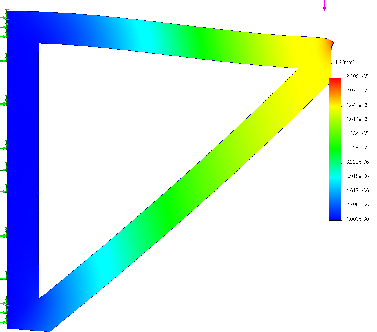
Force Distribution Analysis

Figure 2 | Example of a three-node and three-link truss with a force of 10 N on the $3^{rd}$ node. The $1^{st}$ and $2^{nd}$ nodes are for support and are fixed in the vertical and horizontal directions. This is different than the actual forces and linkages used in the dataset. Simply for visualization.

In a pin‐jointed truss, all external loads applied at the joints are carried solely as axial forces in the members, since the idealized pins prevent bending and shear¹⁸. When a load is applied at a joint, that joint must satisfy both horizontal and vertical equilibrium. For a “V”-shaped truss with two members meeting at a loaded apex, the applied vertical load P splits equally into the two inclined members. The axial force in each member

(5) $\begin{equation*}F_{\text{member}} = \frac{P}{2 \sin \theta}\end{equation*}$

where θ is the inclination angle; their horizontal components cancel, maintaining equilibrium⁸.

More complex trusses follow the same principle at every joint: forces “flow” along member axes, splitting and recombining until they reach the supports. This flow can also be captured by assembling all member contributions into a global stiffness matrix [K] and solving for nodal displacements u in

(6) $\begin{equation*}\bm{K} \, \bm{u} = \bm{F}\end{equation*}$

after which each member force is recovered via its axial stiffness. This can be found using the equation $k=\frac{EA}{L}$ where k is the axial stiffness, E is the Young’s Modulus, A is the cross-sectional area, and L is the length:

(7) $\begin{equation*}F^{e} = k \left( u_{j} - u_{i} \right)\end{equation*}$

This matrix approach enforces equilibrium across the entire structure simultaneously and scales naturally to indeterminate or moving trusses¹⁹.

Methodology

The methodology comprises four principal stages: kinematic path generation, global stiffness matrix assembly, pose‐by‐pose force computation, and dataset construction with validation. Verification and performance assessments are embedded throughout to ensure correct integration and to characterize solver behavior¹.

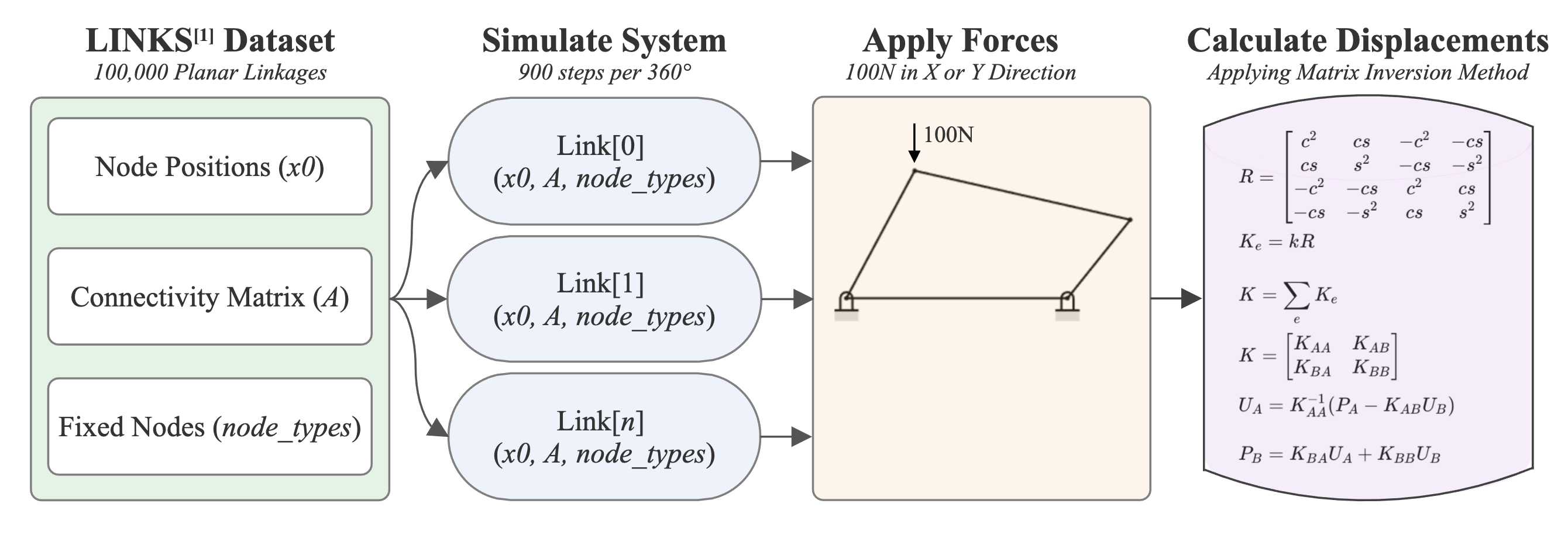
Figure 3 | (1) Gathering information from a dataset of linkages¹. (2) Simulating the motion through 900 discrete steps. (3) Applying a force of 100 N onto a random node in the X or Y Direction. A large force, such as 100 N, is needed to ensure that there is displacement data from the linkage. If the force was 1 N, the displacement data would be much smaller, and in some cases, near 0. (4) Calculating the displacements of the nodes based on the force distribution and applying the Direct Stiffness Method.

Linkage Collection and Input Preparation

The initial dataset comprised one million planar linkage definitions drawn from Nobari et al.’s LINKS repository¹. For each mechanism, three distinct pieces of information were extracted and reformatted for subsequent analysis. First, the two‐dimensional coordinates of every joint were obtained as an N×2 array of (x,y) pairs, where N denotes the number of nodes in the linkage. Second, the connectivity matrix (originally provided as an N×N Boolean array) was converted into a list of element node‐pairs; this adjacency list format specifies exactly which nodes form bar elements and enables efficient assembly of the global stiffness matrix. Third, a Boolean flag vector indicating fixed (support) versus free nodes was transformed into a zero‐based index list of fixed degrees of freedom, allowing straightforward application of boundary conditions in the solver.

In every linkage definition, node 0 is treated as a fixed anchor. The bar connecting node 0 to node 1 serves as the driving link: its prescribed rotation propagates motion throughout the mechanism via the connectivity graph. All data‐format conversions were implemented as pure, in‐place NumPy routines, ensuring that the input arrays for node coordinates, element connectivity, and fixed‐node indices seamlessly feed into the direct‐stiffness solver without additional preprocessing.

Simulating Multi-Nodal Linkage Motion

Each linkage is processed in numerical sequence from the LINKS repository. The rotation of the driving link between node zero and node one is divided into 900 equal steps¹. At every step, the motion solver receives the linkage definition (node positions, element connectivity, and support indicators) and the specified number of increments. The solver returns a three‐dimensional array with 900 slices, each containing the two‐dimensional coordinates of all joints at that instant.

In practice, the mechanism’s input link completes a full circle through these small rotations. For each rotation step j, the simulator enforces the loop‐closure constraints across all moving loops and produces the set of joint coordinates $x_i$ $(\theta_j )$ . This dense sampling captures the smooth evolution of the mechanism’s shape without resorting to iterative numerical integration over time.

Once the coordinates for all 900 poses are obtained, each snapshot is reformatted to match the solver’s input requirements using the input preparation function from 3.1. The two‐dimensional arrays of (x,y) values become the node‐position matrix, and the support flags from Section A identify which joints remain fixed. By treating each snapshot as an independent static configuration, the direct stiffness solver can be applied seamlessly to compute internal forces at every motion step. Consequently, the complete motion of each linkage is transformed into a sequence of static analyses, providing a detailed map of structural performance throughout the cycle.

This approach is used to emphasize the structural analysis of the linkage mechanism over the rotational and torque characteristics. For linkage strength analysis, it is more applicable to use an external force that depicts displacement data than to use a torque and rotation-based approach. A static method also significantly reduces the solver’s computation time while maintaining a high level of accuracy and processing speed.

Structural Model Assembly

For each pose, the current node positions and connectivity define a pin‐jointed truss. Element lengths and orientations are recalculated, and local axial stiffnesses are transformed into the global frame and assembled into a sparse stiffness matrix. Fixed‐node constraints are enforced by eliminating the corresponding degrees of freedom, yielding the reduced stiffness matrix $K_{red}$ .

Pose‐by‐Pose Force Computation

A one‐time LU factorization of $K_{red}$ is performed per mechanism. For each of the 900 poses, the nodal‐load vector is updated to reflect a nominal 100 N coupler force, and the system

(8) $\begin{equation*}\bm{K_{red}} \, \bm{u} = \bm{F}\end{equation*}$

is solved for nodal displacements in under 0.1 ms per pose using sparse‐matrix routines. Member axial forces are obtained by projecting these displacements along each element’s axis.

Data Aggregation and Validation

The original linkage parameters, joint trajectories, nodal displacements, and member force envelopes are consolidated into a searchable database. Validation includes comparison of four‐bar test cases against hand‐computed equilibrium (errors < 1%) and spot‐checks against commercial FEA (discrepancies < 2%). The full dataset and solver code are released under an open source link²⁰ to support reproducibility.

Computational Performance and Scalability

A complete run of all 100,000 linkages on a standard desktop initially overwhelmed available Random Access Memory (RAM), since each pose generated full stiffness matrices, displacement vectors, and force envelopes that together required many gigabytes. To address this, the program was restructured using Dask to process groups of one hundred linkages at a time²¹. Each group’s results were written out to disk before processing the next group, keeping memory data to a minimum. After all groups completed (each requiring 20–30 s), the individual outputs were merged into the final combined dataset. This approach reduced RAM usage by more than 80% and allowed the entire 100,000-linkage workload to complete in about 37 minutes on a mid-range workstation. Because batch size and parallel-worker count can be adjusted freely, the same design can scale to millions of linkages without exceeding a single machine’s memory, relying on disk storage instead of RAM.

Results

The results of such an exhaustive search, encompassing over 100,000 complex linkages, are bound to provide valuable insights into the behavior of these mechanisms when operating under a wide range of loads. The linkages in the data set involve up to 20 nodes and cover a broad range in terms of complexity and configuration, allowing for the thorough study of the interaction between the linkage geometry, the application of forces, and the resulting displacements.

This analysis clearly shows how the number of nodes in a linkage significantly affects its behavior when under load. More nodes in a linkage provide, generally, more complicated patterns of displacement due to the complex manner in which force applied to any one node is transmitted through the structure. This is further reflected in the displacement data, where it was shown that magnitude and direction vary greatly across nodes for more complex linkages.

From these analyses, a common pattern shown is that the position of the force application node and the direction of the applied force are major factors that determine the nature of the overall linkage response. This pattern highlights the occurrence of periphery nodes resulting in a larger displacement.

In the majority of cases, this characteristic is fulfilled; however, the overall displacement of a node relies on multiple factors. These factors include the distance from the connecting nodes, the number of connections to other nodes, and the connectivity distance from the driven node. For example, a node that has a large distance from the primary connecting node will have a large displacement. This holds in the majority of scenarios. However, there are some exceptions. If a node has multiple connections to the nodes around it, the extra support from the additional links decreases the likelihood that it will be displaced by a large amount. We notice here that the nodes lying on or near the periphery of the linkage result in larger overall displacements for forces applied to more centrally located nodes. Very different displacement patterns will result depending on the applied force direction for the linkage configuration. In linkage design, therefore, the magnitude as well as direction of forces is an important consideration.

The dataset further yields valuable insight into the way in which stresses are distributed across the linkage structures. It was noted that specific geometric configurations always result in the concentration of stresses at certain nodes or connections. This becomes especially useful for designers interested in optimizing linkage designs for structural integrity and longevity. Using this knowledge, designers would know where to reinforce the structure or change the geometry to distribute the loads more appropriately.

Figure 4 | Simulation of a 7-node linkage carrying a 100 N load at a random node. The light blue traces show how each bar sweeps through space over 900 small rotations of the driving link (in this image, there are around 50 small rotations for visibility). The solid dark blue outline highlights the linkage’s starting shape. Red arrows point from each joint to its position of maximum displacement, and green circles mark the joints that move the most.

The comprehensive nature of the dataset, containing information on node position, connectivity, force application, and resulting displacements, enables an in-depth analysis of linkage behavior. This rich dataset forms a basis for further research into linkage optimization that can enable superior linkage designs in many applications within robotics and mechanical engineering.

Linkage	Initial X(m)	Initial X(m)	X Displacement (m)	Y Displacement (m)
7 Nodes	0.309	0.585	2.44e-18	8.38e-19
8 Nodes	0.257	0.405	5.01e-18	6.27e-18
10 Nodes	0.0456	1.26	-1.48e-13	-2.57e-14
13 Nodes	0.529094	0.054567	0.005407	-0.002474

Table 1. Change in node positions in multi-nodal linkages with a force of 100 N on a random node. Average displacements are calculated by dividing the sum of all node displacements by the total number of nodes. Measurements that are extremely small numbers have been calculated by the solver to maintain a level of accuracy. In the use case of linkage design, these tend to be effectively 0. All distance and displacement measurements are meters.

Limitations

While the pipeline provides rapid, large‐scale structural insights, it relies on an axial‐only, pin‐jointed truss model and therefore does not capture bending stiffness, joint compliance, or dynamic effects. All analyses assume a uniform 100 N coupler load and linear elastic material behavior, which provides a clear baseline but can be extended in future work to variable loading and non‐linear materials. The study uses a fixed subset of the LINKS repository, which only includes planar, rigid‐body mechanisms. This means that three‐dimensional or compliant linkages fall outside its scope. Finally, although batch processing with Dask enables efficient use of typical desktop resources, further scaling to millions of linkages may benefit from additional optimization or distributed computing infrastructure.

This approach has many strengths in static force‐distribution mapping. However, the current approach omits inertial and dynamic forces, which often dominate in high‐speed or impact‐driven robotic applications. By focusing on static loading, the method remains applicable to mechanisms operating at moderate speeds or under slowly varying loads. Due to this, its predictions may understate stresses in scenarios involving rapid acceleration or vibration. Extending the framework to include dynamic and inertial effects would broaden applicability to high‐speed mechanisms and improve fidelity under transient loading.

Key Contributions

This paper helps to fill this gap by presenting a new method that combines efficient kinematic simulation with robust truss analysis, allowing for a better understanding of linkage behavior for a range of operating conditions. By building on the existing literature in computational inverse kinematics, this paper incorporates crucial aspects of structural integrity and performance optimization into a comprehensive analysis. Key contributions of this paper are:

Development of a Comprehensive Dataset

A dataset of approximately 100,000 2D linkage configurations, analyzed at 900 discrete positions throughout their motion cycles. This dataset combines kinematic data with detailed stress and displacement information, providing a resource for researchers and designers in the field of linkage design.

Novel Integration of Kinematic and Load-based Analyses

By combining efficient kinematic simulation with a robust truss solver, rapid assessment of internal forces and displacements throughout the linkage’s motion cycle can be determined. This provides a more comprehensive understanding of linkage behavior under various load conditions.

Efficient Computational Framework

This enables effective evaluation of stresses on linkages throughout their entire motion, significantly improving upon existing solvers. This framework enables the rapid generation and analysis of a large-scale dataset, potentially accelerating the design and optimization process for linkage mechanisms.

Insights into Linkage Optimization

Identified patterns in force distribution and stress concentration across various linkage configurations. These insights can guide designers seeking to optimize linkages for both kinematic performance and structural integrity.

Future Research Directions

While this study provides valuable insights into how linkage design influences internal stresses, several avenues exist to further enhance the results.

Future research could expand the analysis to larger portions of the LINKS dataset or generate additional linkage configurations. This would offer a more comprehensive view of the design space and potentially reveal further relationships between linkage geometry, motion characteristics, and internal stresses.

Additionally, integrating this stress analysis framework with advanced optimization techniques represents a promising direction. By combining comprehensive stress data with machine learning algorithms, designers could develop linkages that achieve desired motion characteristics while minimizing internal stresses and maximizing structural integrity.

Such advancements are expected to enable the creation of more robust and efficient linkages, applicable across a wide range of robotics and mechanical engineering domains.

Conclusion

The combination of a kinematic motion simulator and direct-stiffness truss solver allows for a comprehensive analysis of multi-nodal planar linkages across their full range of motion. This method generated a dataset of 100,000 1-DOF planar linkages, each annotated with axial force and displacement information, creating a resource for future research and design optimization in robotic mechanisms. Additionally, specific use case data can be created by using the solving algorithm.

The results demonstrate relationships between linkage geometry, motion characteristics, and internal load, illustrating that simultaneous consideration of kinematics and structural response yields more realistic and informative performance predictions than separate analyses. The study confirms that, for the majority of cases, predicted displacement trends correspond with simulation outcomes, validating the methodology.

The analysis also reveals that displacement magnitudes are influenced by node connectivity: nodes with more surrounding connections resist displacement, whereas less connected nodes experience larger movements. Exceptions to general trends are thus explained by structural connectivity rather than positional assumptions.

While the current static approach accurately captures general displacement behavior, future work could incorporate dynamic simulation to account for inertial effects at high speeds. Nonetheless, static predictions closely approximate actual motion for moderate-speed applications.

Overall, this work establishes a framework for analyzing complex linkage systems, providing designers with a rapid, reliable tool for predicting structural response and optimizing designs under varied loading conditions. The dataset and solver offer a foundation for accelerating engineering decision-making and enhancing robotic mechanism reliability.

Discussion

This appendix presents a benchmark of the solver applied to a three-bar right triangle truss. The nodes are located at (0,0), (0,2), and (2,2). Nodes 0 and 1 are fixed, while a vertical load of $F_y=-10N$ is applied at node 2. Each element has cross-sectional area $A=1.0×10^{-6}m^2$ and modulus of elasticity $E=2.0\times 10^9 Pa$ .

For a truss element of length L, area A, modulus E, and direction cosines (c,s), the stiffness matrix is

(9) $\begin{equation*}\bm{k}^{(e)} = \frac{EA}{L}\begin{bmatrix}c^2 & cs & -c^2 & -cs \\cs & s^2 & -cs & -s^2 \\-c^2 & -cs & c^2 & cs \\-cs & -s^2 & cs & s^2\end{bmatrix}\end{equation*}$

The three members yield:

Figure 5. Right triangle truss showing original (blue) and deformed (red) configuration under a vertical load of 10 N at node 3.

With degree-of-freedom ordering $[u_0x,u_0y,u_1x,u_1y,u_2x,u_2y ]$ , the global stiffness matrix is

The external load vector is

(10) $\begin{equation*}\bm{K} =\begin{bmatrix}353.6 & 353.6 & 0 & 0 & -353.6 & -353.6 \\353.6 & 1353.6 & 0 & -1000 & -353.6 & -353.6 \\0 & 0 & 1000 & 0 & -1000 & 0 \\0 & -1000 & 0 & 1000 & 0 & 0 \\-353.6 & -353.6 & -1000 & 0 & 1353.6 & 353.6 \\-353.6 & -353.6 & 0 & 0 & 353.6 & 353.6\end{bmatrix}\end{equation*}$

Boundary conditions fix DOFs of nodes 0 and 1. The reduced system for node 2 is

(11) $\begin{equation*}\bm{F} =\begin{bmatrix}0 & 0 & 0 & 0 & 0 & -10\end{bmatrix}^{T}\end{equation*}$

Solving (11) gives

$K_{AA} =\begin{bmatrix}1353.6 & 353.6 \\353.6 & 353.6\end{bmatrix},\qquad P_{A} =\begin{bmatrix}0 \\-10\end{bmatrix}$

and

$[u_{2x} = 0.01000~\text{m},u_{2y} = -0.03828~\text{m}]$
and

$[||u_2||-\sqrt{u_{2x}^2+u_{2y}^2}=0.03957 m]$

The axial forces are

(12) $\begin{align*}e_{01}: &\quad N = 0.00~\text{N} \\e_{12}: &\quad N = +10.00~\text{N}~(\text{tension}) \\e_{02}: &\quad N = -14.14~\text{N}~(\text{compression})\end{align*}$

Quantity	Value	Interpretation
u_2x	0.01000 m	horizontal displacement
u_2y	-0.03828 m	vertical displacement
∥u_2∥	0.03957 m	maximum displacement
N_01	0.00 N	axial force
N_12	+10.00 N	tension
N_02	-14.14 N	compression

Table 2. Nodal displacements and element forces for the 3-bar truss benchmark under a 10 N vertical load at node 2. Tension is reported as positive, compression as negative.

Stress Analysis and Material Properties

The internal axial forces in each truss member are obtained from the solved nodal displacements. For each element, the axial force $N_i$ is related to the axial stress $\sigma_i$ by

(13) $\begin{equation*}\sigma_i = \frac{N_i}{A}\end{equation*}$

where A is the cross-sectional area of the bar.

The material used in this benchmark model is assumed to be linearly elastic with Young’s modulus $E=2.0×10^9Pa$ and cross-sectional area $A=1.0×10^{-6}m^2$ . These values are representative of lightweight polymeric material. Table 2 summarizes the adopted material properties.

2.0\times 10^9 Pa — Table 3. Material and section properties assumed for the 3-bar truss benchmark. Values define axial stiffness $EA\/L$ used in the stiffness method.

Using the computed displacements, the axial forces in each member are listed in Table 3. Tension is reported as positive, and compression as negative.

Member	Force (N)	Stress (MPa)	Mode
0–1	0.00	0.00	–
1–2	+10.00	+10.00	Tension
0–2	-14.14	-14.14	Compression

Table 4. Axial forces and corresponding stresses in each truss member, computed from solved nodal displacements. Stresses are normalized by cross-sectional areas.

References

A. H. Nobari, A. Srivastava, D. Gutfreund, K. Xu, F. Ahmed. LInK: Learning joint representations of design and performance spaces through contrastive learning for mechanism synthesis (2024). [↩] [↩] [↩] [↩] [↩] [↩] [↩]
S. Enrique, P. Carlos, R. Higinio. Mathematical dimensional synthesis of four-bar linkages based on cognate mechanisms. Mathematics 13 11 (2025). [↩] [↩]
L. W. Kam, S. Li, H. S. Park. Eighty years of the finite element method: Birth, evolution, and future. Archives of Computational Methods in Engineering 29 4431–4453 (2022). [↩] [↩] [↩]
L. Sumin, J. Jihoon, N. Namwoo. Deep generative model-based synthesis framework of four-bar linkage mechanisms with target conditions. Journal of Computational Design and Engineering 11 (5) (2024). [↩]
A. G. Erdman. Three and four precision-point kinematic synthesis of planar linkages. Mechanism and Machine Theory 16 375–387 (1981). [↩]
W.R. Kim, J. Jung, J. U. Ha, D. Lee, J. K. Shim. Data-Driven Dimensional Synthesis of Diverse Planar Four-bar Function Generation Mechanisms via Direct Parameterization. (2025). [↩]
J. Unde, Y. Ito, J. Colan, Y. Hasegawa. Kinematic analysis and experimental verification of transforming planar linkage mechanism. Robomech Journal 2(5), 289–302 (2025). [↩]
R.C. Hibbeler. Engineering Mechanics: Statics & Dynamics Pearson (2017). [↩] [↩]
C. A. Fellipa. A historical outline of matrix structural analysis: a play in three acts. Computers & Structures 79(17), 1313–1324 (2001). [↩]
E. Anderson, Z. Bai, C. Bischof, S. Blackford, J. Demmel, J. Dongarra, J. Du Croz, A. Greenbaum, S. Hammarling, A. McKenney, D. Sorensen. LAPACK Users’ Guide. SIAM (1999). [↩]
L. Zheng, K. Karapiperis, S. Kumar, D. M. Kochmann. Unifying the design space and optimizing linear and nonlinear truss metamaterials by generative modeling. Nature Communications 14 7563 (2023). [↩]
J. Feng, C. Li, Y. Xu, Q. Zhang, F. Wang, J. Cai. Analysis of key elements of truss structures based on the tangent stiffness method. Symmetry 12, no. 6: 1008 (2020). [↩]
R. Sedaghati. Benchmark case studies in structural design optimization using the force method. International Journal of Solids and Structures 42(21), 5848–5871 (2005). [↩]
S. Walbrun, C. Witzgall, S. Wartzack. A rapid CAE-based design method for modular hybrid truss structures. Design Science 5 (2019). [↩]
D. Sachau, R. Schwertassek. Multibody simulation of a truss structure using finite element results. WIT press (1996). [↩]
Š. Ondočko, J. Svetlík, R. Jánoš, J. Semjon, M. Dovica. Calculation of Trusses System in MATLAB—Multibody. Applied Sciences 14(20), 9547 (2024). [↩]
V. Plevris, A. Ahmad. Deriving Analytical Solutions Using Symbolic Matrix Structural Analysis: Part 2 – Plane Trusses. arXiv preprint, 11 (4) (2024). [↩]
F. D. Beer, E. R. Johnston, J. T. DeWolf, D. F. Mazurek. Mechanics of Materials. McGraw-Hill Education (2014). [↩]
A. Kassimali. Matrix Analysis of Structures. Cengage Learning (2022). [↩]
GitHub. Arnav-Gaddamanugu/research: A Python toolkit for large‐scale planar linkage analysis that combines 900‐step kinematic sampling with direct‐stiffness truss solves, batch‐processed via Dask to produce a 100 000-linkage force-annotated dataset in under an hour on commodity hardware. https://github.com/Arnav-Gaddamanugu/research (2025). [↩]
Dask: Library for dynamic task scheduling. http://dask.python.org(2014). [↩]

Property	Value
Young’s modulus $E$	$2.0\times 10^9 Pa$
Cross-sectional area $A$	$1.0 \times 10^{-6} m^2$
Density $\rho$	Not specified
Poisson’s ratio $\nu$	Not specified

Simulation of Linkages and Trusses: Predicting Force Distribution and Mechanical Behavior

Abstract

Introduction