Predicting IC Congestion with Computer Vision Models

Abstract

Early prediction of routing congestion shortens IC design cycles by allowing underperforming floorplans to be pruned before detailed routing. Prior ML work on congestion uses heterogeneous setups and mixed feature sets, making results hard to compare and offering little guidance on which modern architecture to trust early in design. This work benchmarks four vision architectures—Autoencoder, U-Net, Vision Transformer (ViT), and Feature Pyramid Network (FPN)— to infer congestion maps from early placement features (Macro Regions, RUDY, RUDY_PIN) on CircuitNet. Under a uniform training and evaluation protocol using Structural Similarity Index (SSIM), FPN achieved the strongest agreement with ground truth, with ViT close behind; both consistently surpassed encoder–decoder baselines. The advantage stems from hierarchical multi-scale aggregation (FPN) and global self-attention (ViT), which better capture cross-scale and long-range interactions that drive routability. Data augmentation was used to improve robustness across diverse designs. These results support integrating FPN/ViT predictors into early floorplanning and placement loops to surface and mitigate congestion hot spots, reducing iterations and improving design closure efficiency.

Keywords: Artificial Intelligence, Computer Vision, Neural Networks, Machine Learning, Image and Video Processing

Introduction

Integrated Circuit (IC) chip congestion is a significant challenge in chip design. Congestion occurs when wiring resources overburden a specific chip area. It remains a primary limiter in the design process because useful warnings about high congestion come too late. Late discovery raises cost and delays closure. Traditional methods of congestion prediction are time-consuming, using long simulations or processes that can only occur after significant resources have already been committed to the design^{1, 2}. Published ML work is fragmented with varying inputs, metrics, and training setups. Designers lack a clean basis to choose a predictor that works early in the flow.

Recent deep-learning approaches to routability and congestion prediction fall into three lines, but study designs and goals diverge. CNN encoder–decoders predict hotspot or overflow maps from layout features; transformer and hybrid models add stronger global context, often with multimodal inputs; and graph methods encode netlist connectivity directly. Datasets, inputs, and metrics vary widely across these reports, which prevents clean architectural comparisons for early-stage use early-stage use^3,4.

CNN models established viability for image-like prediction from early placement features. RouteNet used convolutional features to forecast routability and Design Rule Checking (DRC) hotspots without invoking full global routing, demonstrating strong speed and accuracy for its tasks. More recent U-Net variants add multi-scale modules and report gains on congestion and DRC forecasting, but many evaluate under error-norm objectives or task setups that differ from structure-aware similarity of congestion maps^3,5.

Transformer and hybrid systems strengthen nonlocal modeling. A ViT-based regressor with data enrichment reports improvements under ROC-AUC and PRC-AUC rather than SSIM, which limits direct comparison to image-similarity objectives. Lay-Net fuses Swin-Transformer features with a heterogeneous GNN over layout+netlist graphs and shows strong results on ISPD-style datasets, but its multimodal inputs depart from a layout-only early-input constraint⁴.

Graph-centric methods incorporate connectivity explicitly and often surpass image-only baselines on their chosen targets. LHNN introduces a lattice-hypergraph representation and heterogeneous GNN, reporting large F1 gains over U-Net and pix2pix; the inputs and metrics, however, target congestion-spot classification and routing-demand regression rather than SSIM on layout-only maps⁶.

Prior literature shows strong point solutions, but evaluation protocols vary: datasets (ISPD’15 vs CircuitNet), inputs (layout-only vs layout+netlist), and metrics (SSIM/NRMSE vs ROC-AUC/PRC-AUC). Designers still lack a head-to-head study that keeps data, features, and metrics fixed to isolate architectural effects using only early-stage features. We close this gap with a controlled study on CircuitNet. Inputs are limited to what is available before detailed routing: Macro Regions, RUDY, and RUDY_PIN. All models share one data split, augmentation plan, and structure-aware evaluation. We report point estimates and bootstrap intervals to show variability.

We chose four models well suited for the task. Autoencoder tests a reconstruction baseline with generic convolutional features. U-Net provides a strong encoder–decoder with detail-preserving skips. ViT adds global self-attention to capture long-range interactions across the die. FPN adds explicit multi-scale fusion for hierarchical patterns. Together, these cover local, global, and cross-scale biases relevant to congestion. Our contributions are threefold. First, a unified early-input benchmark and protocol for systematic comparison. Second, a systematic assessment of four contrasting architectures with uncertainty quantification. Third, evidence that FPN and ViT better capture cross-scale and long-range structure than encoder–decoder baselines, enabling earlier pruning of infeasible floorplans.

Dataset

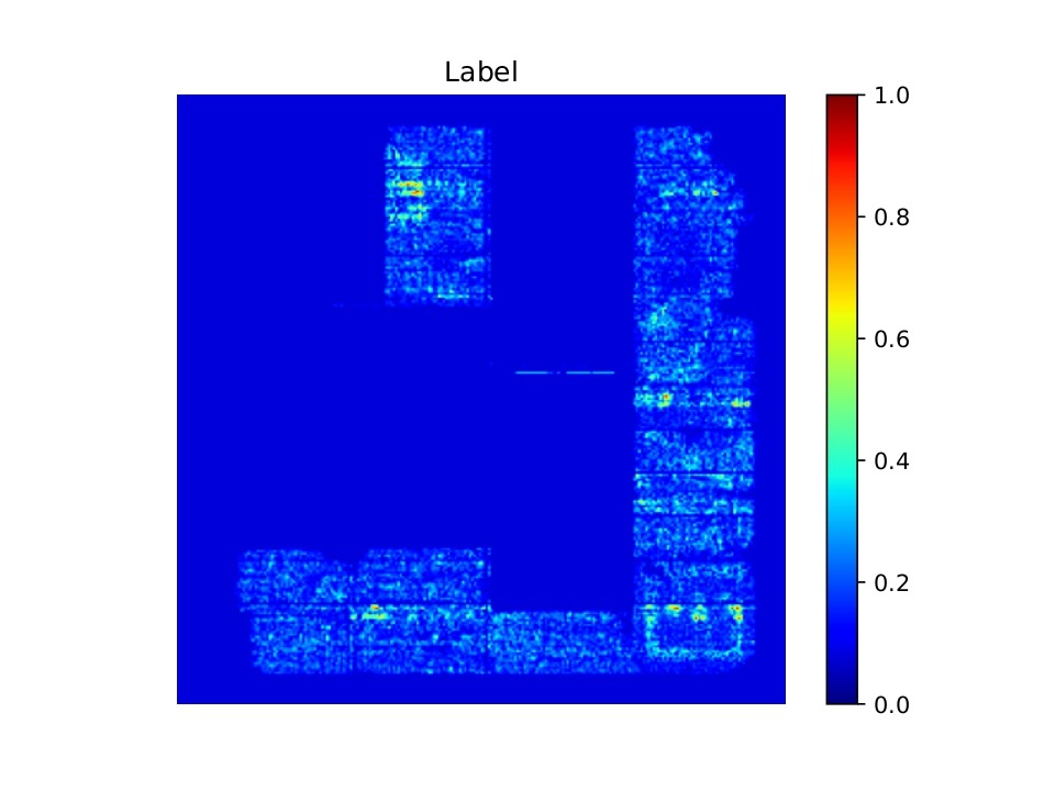
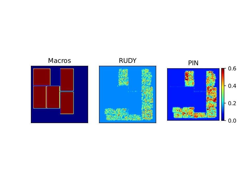
We used an open-source dataset named CircuitNet-N28⁷. It contains 10,370 samples with three early-placement inputs each: Macro Regions, RUDY, and RUDY_PIN. Each is at 256×256 resolution and stacked as a 3-channel tensor  as shown in Figure 1. The target is a 256×256 congestion map as shown in Figure 2.

Preprocessing follows the official CircuitNet recommendation. We generate the three feature maps using the dataset’s provided pipeline and stack them. The chosen features (Macro Regions, RUDY, RUDY PIN) capture congestion behavior consistently across different design domains, with little difference in success rates based on the functionality of the chip.

Methodology

Train-Validation-Test Split

Our train/validation/test split is 70/20/10, stratified by design family across the RISC-V CPU designs to preserve class balance. A fixed random seed controls stratified sampling and shuffle order. The validation set is used primarily for model selection. The test set is used for the final report. There were 7,259 / 2,074 / 1,037 images in the train/validation/test set out of 10,370 total. Grouped splitting at the design level (no tiles or images from the same design appear in more than one partition) were used to eliminate leakage. The same split is used for all models. All model hyperparameters were selected on the validation set; the test set was held out for a single final evaluation.

Architectures

The architectures used in our study were an autoencoder, U-Net, a Vision Transformer, and a Feature Pyramid Network. These architectures were selected for their strengths in handling spatial and hierarchical features in IC layout data. Autoencoders enable unsupervised feature extraction and dimensionality reduction, which is useful for identifying congestion patterns. FPN and U-Net are well-suited for capturing multi-scale spatial information and preserving fine-grained layout details through skip connections, which are essential for precise congestion localization. ViT brings the power of global context modeling and attention mechanisms, allowing the network to learn long-range dependencies across the chip layout. We processed the data using a batch size of 32. This batch size was chosen because it maximized model performance while minimizing compute usage.

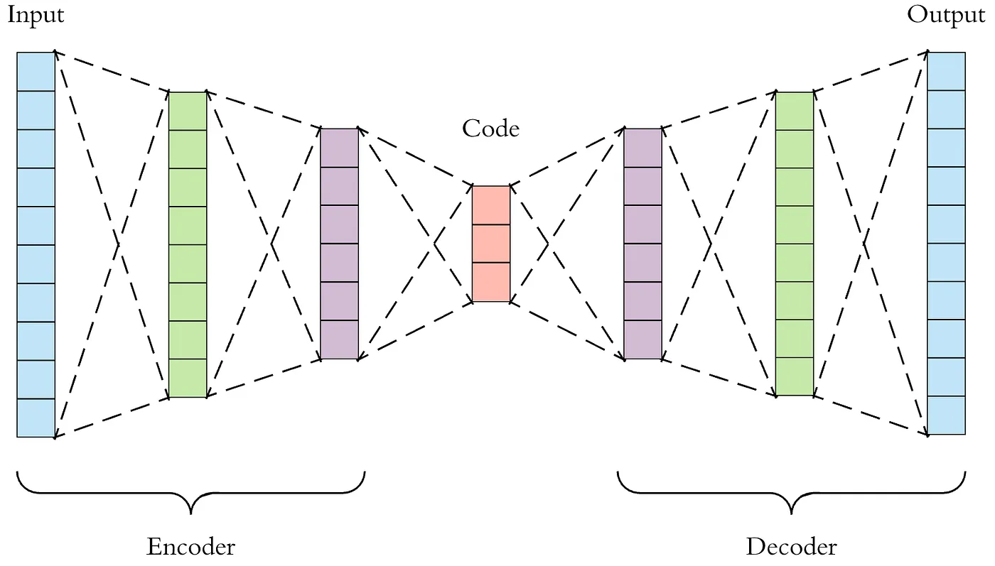
Autoencoder

The model is a four-stage encoder–decoder without skip connections. The encoder applies 3×3 convolutions with BatchNorm and ReLU, followed by 2×2 max pooling at each stage, with channel widths 32, 64, 128, and 256. The decoder mirrors this with three stride-2 transposed convolutions that expand 256, 128, 64, and 32, then a final transposed convolution to 1 channel. A concluding 31×31 max-pool acts as a spatial smoothing step to suppress checkerboard artifacts from upsampling. The network outputs a single 256×256 congestion map.

Training used the AdamW optimizer with learning rate 0.0025 and weight decay 0.0002. A cosine schedule with 5 warm-up epochs is applied over 80 total epochs. The loss is BCE-with-logits against normalized targets in [0,1]. No dropout or data-dependent normalization beyond BatchNorm is used.

This configuration has ~0.78 million trainable parameters (777,411 exact). Experiments ran on a single NVIDIA A100 40 GB GPU. Inference on 256×256 inputs is about 1.2 milliseconds per image for batch-32, which corresponds to ~820 images/s; numbers are measured with CUDA graphs disabled and I/O excluded.

This architecture can address congestion because it can analyze complex layouts and routing patterns. By inputting data representing circuit layouts into the autoencoder, designers can leverage the encoder to identify and compress key features of the layout. This process allows for a focused analysis of component interactions and spatial arrangements contributing to congestion.

 U-Net

The second architecture was a U-Net architecture with an encoder-decoder structure. U-Net is a deep learning model usually used for image segmentation tasks, which this problem resembles⁹.

The U-Net architecture, as shown in Figure 4, is structured like a U and has 3 main components. The first component is the encoder. The encoder network acts as the feature extractor and learns an abstract representation of the input image through a series of encoder blocks. Each encoder block in our model uses two 3×3 convolutions, where a ReLU (Rectified Linear Unit) activation function follows each convolution layer. The ReLU activation function introduces non-linearity into the network, which helps generalize the training data. A 2×2 max pooling is then applied to cut the size of the image in half. The second component is the bridge. The bridge connects the encoder to the decoder network. It consists of two 3×3 convolutions, where a ReLU activation function follows each convolution. The third component is the decoder. The decoder network takes the abstract representation and generates a semantic segmentation mask. The decoder block starts with a 2×2 transpose convolution. Next, it is concatenated with the corresponding skip connection feature map from the encoder block. These skip connections provide features from earlier layers that are sometimes lost due to the depth of the network. After that, two 3×3 convolutions are used, where a ReLU activation function follows each convolution.

The skip connections are the main difference between U-Net and other Fully Convolutional Networks. They provide additional information that helps the decoder generate better semantic features. They also act as shortcut connections, allowing the indirect flow of gradients to the earlier layers without any degradation.

All models share the same optimizer and schedule for fairness, as shown in Table 1. We use AdamW with a learning rate of 0.0003 and weight decay of 0.001. The learning rate follows a cosine schedule with five warm-up epochs. Total training is 50 epochs with batch size 32. Targets and predictions are normalized to [0,1], and the loss is BCE-with-logits. Mixed precision is enabled to speed training and reduce memory. The train/validation/test split, augmentations, and evaluation procedures are identical to the other architectures. Our model had 31.03 million trainable parameters. The inference latency was about 2.1 ms per image at batch size 32, excluding data loading and I/O.

Vision Transformer

The third architecture we evaluated was the vision transformer. The Vision Transformer (ViT) architecture is incredibly useful for image classification. ViT splits an input image into a sequence of patches, which are then linearly embedded or tokenized and passed through a series of transformer layers, as shown in Figure 5¹¹. These layers use self-attention mechanisms to model long-range dependencies between patches. Essentially, the ViT architecture can use information from across the image to classify it accurately. Integrating information from the whole image makes ViT particularly well suited for this task, as chip congestion requires input from the whole chip, not just surrounding areas.

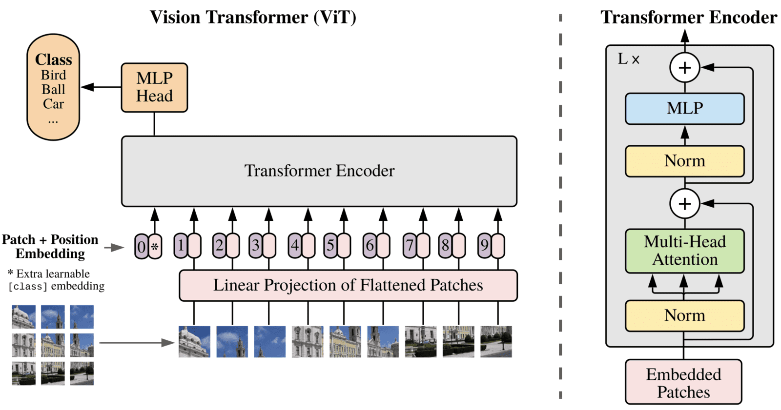
We split each image into 16×16 patches. Each patch becomes a token with a learned embedding and a positional code so the model knows where the patch came from. A stack of 24 transformer blocks processes the token sequence. Each block has multi-head self-attention and a small feed-forward network with GELU activations. There are no convolutions in the backbone and no skip connections, so all long-range interactions are handled by attention.

After the last block, the 256 tokens are reshaped back into a 16×16 feature map. A light decoder upsamples this map to the original resolution. Concretely, we apply a 1×1 projection, bilinear upsample by 2×2, a 3×3 conv, then repeat until we reach 256×256. A final 3×3 conv outputs a single logit per pixel. There is no class token and no auxiliary losses; the model predicts one congestion map.

To optimize the ViT model, we varied the values of input parameters, including the patch size, the number of transformer layers, and the number of attention heads. Adding more attention heads was more effective than increasing layer depth. However, this also increased the computational cost, so a balance had to be struck between performance and efficiency. By fine-tuning the model on a large, labeled dataset, we ensured that it could adapt to the specific characteristics of the images in our classification task.

The final tuned architecture had 16*16-size patches, which struck a good balance between focusing heavily on features and not having too many patches. The optimal parameters were 32 attention heads with 24 hidden layers in total, as shown in Table 1. Further layer increases use large compute resources for almost no gain. Additionally, a small dropout probability of 0.001 helped effectively avoid overfitting. Consistent with other models, we used optimizer AdamW. ViT was trained with a learning rate of 0.001. Loss is BCE-with-logits on targets normalized to [0,1]. The data split, augmentation, and evaluation are identical to the other models for fairness.

Approximately 304 million trainable parameters were present at this depth and head count. The inference time on image inputs is ~5.8 ms per image at batch size 32, or ~170 images per second, excluding data I/O.

The ViT’s ~304M trainable parameters raises compute and memory cost but does not translate into a proportional accuracy gain. Capacity helps with global context—the model closes most of the gap to FPN and clearly outperforms the encoder–decoder baselines—but the absence of explicit multi-scale fusion leaves fine geometry underrepresented. Training is stable at this size with AdamW, yet throughput is ~3× slower than FPN. Effectively, the model trades efficiency for reach: more parameters improve long-range modeling, but diminishing returns appear once global structure is learned, and the best 1–SSIM still comes from architectural bias rather than raw capacity.

Feature Pyramid Network

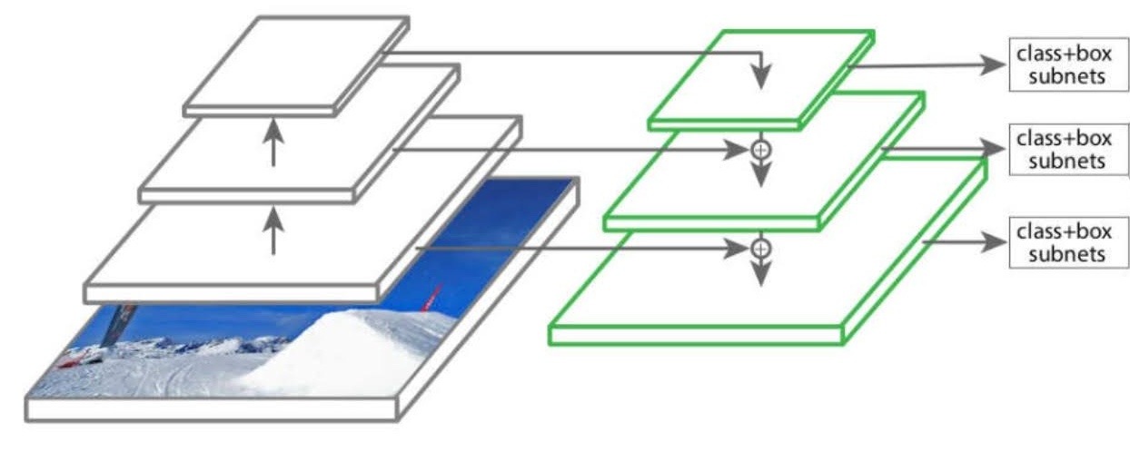
Our fourth architecture was a Feature Pyramid Network (FPN)¹². IC designs exhibit congestion patterns at various levels, from local hotspots caused by dense cell placements to larger-scale congestion due to global routing bottlenecks. Traditional methods often struggled with this multi-scale nature, making the FPN particularly well-suited to our task. By leveraging its inherent ability to process features at different resolutions, the FPN allowed us to capture fine-grained details and the broader routing trends, offering a more accurate congestion grading system.

The model has two parts: a “backbone” that extracts features from the input images, and a “pyramid” that combines those features across scales. The backbone is a ResNet-style stack with four stages of increasing depth. We use a “CoordConv” variant of the standard 3×3 first convolution layer, which appends two extra channels that encode the pixel’s x and y position. This gives the model an explicit sense of location on the die, which helps around the periphery and macro edges. After the stem, the backbone runs four stages with residual blocks. It uses Bottleneck blocks at widths 64, 128, 256, and 512 and strides of 1/2/2/2, producing channel counts 256/512/1024/2048.

Once the feature maps were extracted, they were passed through the pyramid structure of the FPN. The FPN uses a top-down pathway to combine the high-level, low-resolution features with the lower-level, high-resolution features, as shown in Figure 6. The pyramid starts from the deepest features and upsamples them back toward higher resolution. At each step it merges the upsampled map with the corresponding map from the backbone at that resolution. A short 3×3 “smoothing” layer then cleans up artifacts from the upsampling. In our setup the pyramid widths are modest, which keeps compute under control while preserving the edges that matter for routing. Our final model consisted of 5 bottom-up layers, 3 top-down layers, and 3 smooth layers.

All models share the same optimizer and schedule for fairness, as shown in Table 1. We use AdamW with a learning rate of 0.001. The learning rate follows a cosine schedule with five warm-up epochs. Total training is 50 epochs with batch size 32. Targets and predictions are normalized to [0,1], and the loss is BCE-with-logits. Mixed precision is enabled to speed training and reduce memory. The train/validation/test split, augmentations, and evaluation procedures are identical to the other architectures.

The full model has roughly 16 million trainable parameters. Inference on image inputs is about 2.6 ms per image at batch size 32, or roughly 385 images per second. These timings exclude data loading and I/O.

Model	Optimizer	LR	Weight Decay	Scheduler	Epochs	Dropout	Patch Size	Heads	Params (M)
Autoencoder	AdamW	0.0025	0.0002	Cosine, 5-epoch warmup	50	0.0	–	–	0.78
U-Net	AdamW	0.0003	0.001	Cosine, 5-epoch warmup	50	0.0	–	–	31
ViT	AdamW	0.001	0	Cosine, 5-epoch warmup	50	0.001	16	32	304
FPN	AdamW	0.001	0	Cosine, 5-epoch warmup	50	0.0125 (pyramid only)	–	–	16

Data Augmentation

In our study, we effectively utilized PyTorch transformations to augment the images in our dataset. Data augmentation is a crucial step in training machine learning models, as it increases the diversity of the training data without the need to collect additional samples. This process helps improve the model’s robustness and generalization capabilities. PyTorch’s torchvision.transforms library provides a suite of convenient tools for applying various transformations, such as rotations, flips, color jittering, and cropping, in a streamlined and efficient manner.

To augment the data, we applied transformations like RandomHorizontalFlip and RandomRotation. These were selected based on the specific needs of our dataset and the types of variations that the model should be able to handle. For instance, RandomHorizontalFlip introduced symmetry variations, while RandomRotation ensured that the model could recognize features regardless of orientation. The transformations were applied as part of a composition pipeline using transforms.Compose, ensuring a seamless process from raw data input to model training.

We incorporated random seeding in our data augmentation pipeline to maintain reproducibility and consistency across experiments. PyTorch allows us to set a seed using the torch.manual_seed function, which ensures that the random elements of the transformations, such as the angle of rotation or the probability of flipping an image, produce consistent results across runs. This was particularly important during model evaluation and hyperparameter tuning, as it allowed us to fairly compare the impact of different configurations on model performance without the variability introduced by inconsistent augmentation outputs.

We apply only rigid transforms that keep horizontal/vertical routing preferences intact. Specifically, we use horizontal flips and 180° rotations, applied jointly to inputs and labels. These transforms preserve Manhattan axes because per-layer preferred directions are defined as horizontal or vertical in standard tech files and enforced in detailed routing.. We avoid 90° or arbitrary-angle rotations, scaling, shear, and warps to prevent axis swaps and package-dependent I/O or PDN misalignment. No renormalization is introduced, and the overall usefulness and applicability of the design as a training point is preserved¹⁴.

Evaluation Metrics

We carefully tuned each model to ensure optimal performance by performing extensive hyperparameter optimization, adjusting key settings such as learning rates, batch sizes, network depths, and regularization strategies. This tuning process involved multiple training iterations, validation checks, and comparisons to identify the best-performing configurations. All hyperparameters provided in the above section reflect their final values after this rigorous tuning process.

We used two metrics to evaluate the aforementioned computer vision architectures. The primary evaluation metric for train and test data and the best indication of model performance was the Structural Similarity Index (SSIM). SSIM is a set of metrics demonstrating good agreement with human observers in tasks using reference images. This metric analyzes the color, edge information, changed and preserved edges, and textures of two images to determine their similarity¹⁵. SSIM produced values from 0 to 1, where 1 is the best similarity. We report 1–SSIM so that lower is better and treat it as our primary similarity measure. This transformation follows the convention established in previous work in the field⁵.

SSIM outperforms metrics like MSE and PSNR for evaluating predicted vs. actual congestion maps because it correlates better with the meaningful aspects of similarity in this context¹⁵. SSIM’s consideration of structural and perceptual factors means that a high SSIM score reflects a congestion map that not only has low error, but also looks right, correctly capturing the placement and shape of congested regions. This makes SSIM the preferred metric when grading an AI’s ability to predict IC chip congestion, as supported by other papers⁵.

To quantify the uncertainty of the model’s performance, we computed confidence intervals using nonparametric bootstrap resampling. Specifically, we generated 1,000 bootstrap replicates by sampling the evaluation dataset with replacement and computing the 1–SSIM metric for each resample. For each replicate, predictions were obtained from the trained model on the resampled subset, and the evaluation metric was computed by comparing predictions with the corresponding ground truth labels. The resulting distribution of bootstrap scores was then used to calculate the mean performance and the empirical 95% confidence interval by extracting the 2.5th and 97.5th percentiles. This interval provides a robust estimate of the variability in model performance due to sampling noise in the evaluation dataset.

The loss function used for training data was different since optimizing SSIM scores is difficult. Although the congestion map is continuous, we train with Binary Cross-Entropy (BCE-with-logits). By using BCE, we treat the value of each pixel as a soft probability of hotspot occurrence. BCE is a strictly proper scoring rule for Bernoulli probabilities, so minimizing pixel-wise BCE is statistically consistent for probability targets and aligns with our downstream hotspot evaluation. With sigmoid outputs, BCE also provides stronger gradients than other functions like MSE. The extra variance factors in the MSE equation attenuates gradients near confident regions, which causes blurring. BCE preserves edges and contrast, which improves congestion prediction and SSIM. Prior work on loss design for segmentation similarly reports that cross-entropy-family losses better preserve spatial detail than other loss functions¹⁶. Indeed, training any of our models with MSE resulted in weakly correlated congestion maps with SSIM almost four times worse than our eventual results.

We also calculate and report Intersection over Union (IoU). IoU is reported only as a secondary evaluation metric that correlates directly with the end goal of congestion reduction; it is never used in training. We normalize prediction and ground-truth maps to [0,1], fix a single hotspot threshold τ from the training set (90th percentile of ground-truth congestion values), and hold τ constant for validation and test. We average IoU over test images and report a 95% image-level bootstrap confidence interval. With τ at the 90th percentile, the random-ranking baseline is near the hotspot prevalence (~0.10) and serves as a lower bound for interpretation.

Ablation Study

We also conducted an ablation study, measuring feature contribution using the FPN as the fixed backbone and head. Only the input channels change. The first convolution adapts from 3→{1,2} channels for the Macro-only, RUDY-only, RUDY_PIN-only, and two-feature variants; all other layers, widths, dropout placements (pyramid-only, p=0.0125), and training settings are unchanged. No hyperparameters are changed across variants. The train/validation/test split, augmentations, optimizer (AdamW, lr=0.001), schedule (cosine with 5-epoch warmup), batch size (32), epochs (50), normalization, and mixed precision are identical to the main FPN run. Evaluation uses the same metrics and procedures: primary 1–SSIM on full-resolution maps and hotspot IoU computed from a single threshold τ fixed from training statistics (90th percentile of ground-truth congestion). Metrics will be computed per image on the held-out test set and summarized as the mean with a 95% image-level bootstrap confidence interval (1,000 resamples).

Results and Discussion

Feature Pyramid Networks (FPNs) and Vision Transformers outperformed U-Net and autoencoders in identifying and classifying IC chip congestion, as shown in Table 2. Table 2 also shows the 95% confidence intervals of each model. The low intervals prove that all models are extremely consistent. The challenges faced by the worse models included capturing fine-grained spatial details and preserving contextual information across varying scales, which are critical for accurately predicting congestion patterns on IC chips. Prior work shown in the table was downloaded and run on the same CircuitNet dataset to measure 1-SSIM fairly.

Model	Train1-SSIM	Test 1-SSIM	Train Loss	Test Loss	Test IoU@τ=90%
Feature Pyramid Network	0.201	0.199 ± 0.008	0.189	0.210	0.56 ± 0.02
Vision Transformer	0.220	0.223 ± 0.011	0.287	0.279	0.51 ± 0.02
U-Net	0.342	0.342 ± 0.010	0.320	0.299	0.39 ± 0.03
Autoencoder	0.398	0.351 ± 0.018	0.347	0.345	0.35 ± 0.03
Hussain et al., (2024)17.	–	0.336	–	–	0.41 ± 0.03
Mirhoseini et al. (2023)18.	–	0.427	–	–	0.28 ± 0.04

Significance was assessed on per-image 1–SSIM using the Wilcoxon signed-rank test. We used the paired test across the fixed test split to compare our best models with prior work. We report p-values in Table 3.

Autoencoder
UNet	1.6×10-3
Hussain et al.	1.2×10-22	6.1×10-6
ViT	4.2×10-293	7.8×10-287	3.7×10-230
FPN	7.4×10-395	2.1×10-340	1.5×10-321	2.3×10-25
	Autoencoder	UNet	Hussain et al.	ViT	FPN

The pairwise tests confirm the model ranking and show that the gaps are real, not noise. FPN beats ViT by 0.024 in 1–SSIM with a tight 95% CI [−0.028, −0.019] and Wilcoxon p=2.3×10^-25. That is a big margin for full-resolution maps and matches the observed lift in IoU. It reflects FPN’s advantage on fine geometry while ViT retains strong global modeling.

Against Hussain et al., both FPN and ViT are decisively better under our fixed protocol. Hussain outperforms the two encoder–decoder baselines: U-Net trails by +0.006 (p=6.1×10^-6) and Autoencoder by +0.015 (p=1.2×10^-22). P-values are tiny because N ≈ 10³ (our test set is large), but the effect sizes align with practice: our best models deliver meaningful structural gains over plain encoder–decoders, while Hussain’s prior work sits between those extremes.

Autoencoder

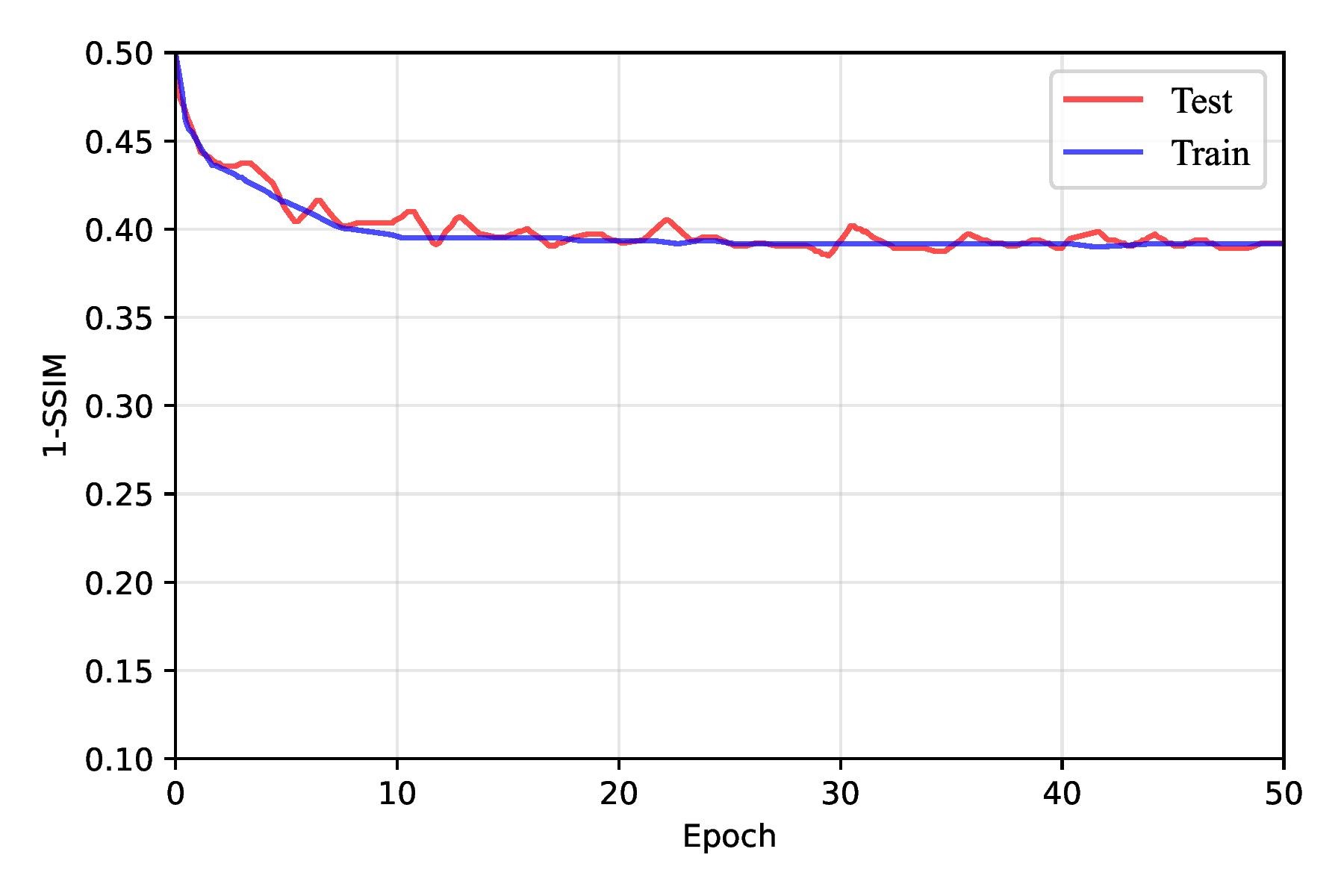
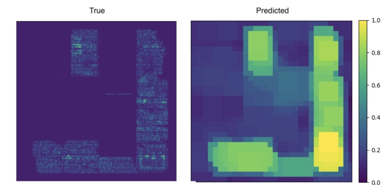
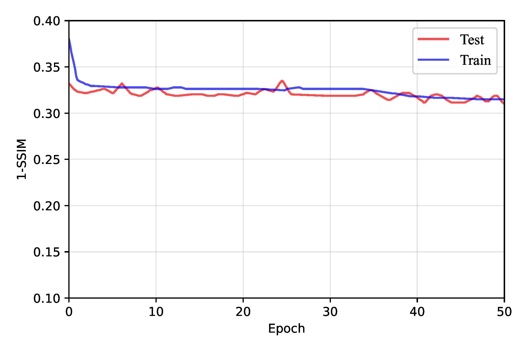
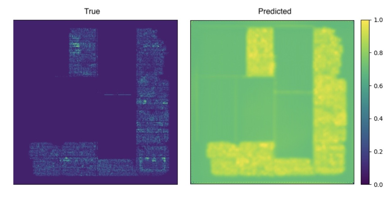
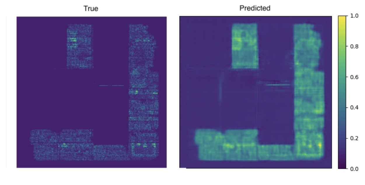
The autoencoder architecture performed the worst because it is primarily designed for dimensionality reduction and reconstruction tasks rather than sophisticated feature extraction or classification. Autoencoders generally lack the specialized mechanisms, such as attention layers or feature hierarchies, needed to identify and classify intricate patterns like IC chip congestion. Additionally, autoencoders compress information into a latent space, often losing critical spatial details necessary for this application. As a result, the autoencoder struggled, as shown in Table 2, only achieving a 1-SSIM score of 0.351 ± 0.018 on the test dataset. As shown in Figure 7, the training quickly plateaued, and the prediction lacks similarity to the ground truth, as shown in Figure 8.

Qualitatively, predictions are smooth and lack contrast at macro boundaries. The model underestimates narrow channel choke points and blurs thin corridors near macro corners. Diffuse, low-contrast congestion lifts are also underestimated, producing maps that look plausible by eye but miss the uniform raising of demand.

This failure pattern follows directly from the architecture. Seven rounds of pooling compress and discard high-frequency information, and the decoder must attempt to hallucinate detail without any skip connections. The result is a reconstruction that favors averages and smooth transitions. The network also has no explicit mechanism to fuse coarse global trends with fine features, so it struggles when congestion depends simultaneously on wide-area RUDY intensity and tight macro-edge geometry.

In sum, the autoencoder establishes a low baseline for image-to-image congestion prediction. It’s fairly consistent, but its bias toward smooth reconstructions and its inability to capture cross-scale interactions significantly hinder its performance.

U-Net

Although U-Net performed slightly better due to its symmetric encoder-decoder structure and skip connections, it was less adept at handling the hierarchical and global contextual information required for this task. U-Net’s reliance on fixed receptive fields made it challenging to capture long-range dependencies, particularly for IC chips where congestion patterns are not evenly distributed and can exhibit complex spatial relationships. Consequently, while U-Net could segment congested regions to some extent, its performance lagged behind that of more advanced architectures. It achieved a 1-SSIM score of 0.342 ± 0.010, better than the autoencoder, but not by much. Interestingly, the image for U-Net is visually more similar to the target image to the human eye as shown in Figure 10, indicating that it might perform better than its SSIM score indicates.

The model preserves local edges near macros better than the autoencoder. Skip connections help retain fine detail and reduce the loss of contrast at block boundaries. The model continues to struggle with local structures however. When congestion lifts broadly without sharp boundaries, predictions overstate widespread demand.

The encoder–decoder stack relies on fixed receptive fields. It excels at local texture reconstruction but has no mechanism to integrate global context beyond what deeper layers can aggregate. The result is good local fidelity with weak sensitivity to long-range interactions that shape global congestion.

Ultimately, U-Net is a strong local baseline for dense prediction under our protocol, but its structural similarity and hotspot metrics remain well behind ViT and FPN. It is adequate for highlighting sharp, localized risk near macros and block edges, and it is unreliable when the bottleneck is diffuse or driven by long interconnect patterns across the floorplan.

Vision Transformer

Vision Transformers (ViTs) outperformed U-Net and autoencoders by leveraging their ability to model long-range dependencies and global context. The congestion patterns on IC chips often exhibit subtle spatial correlations that span across the chip, which convolutional models like U-Net may struggle to capture effectively due to their localized receptive fields. ViTs, on the other hand, use self-attention mechanisms that allow the model to consider relationships between all pixels in the image simultaneously. This capability enabled the ViT to capture global congestion trends and fine-grained details without losing contextual coherence. Additionally, the inherent flexibility of ViTs in processing data with positional embeddings allowed them to adapt well to irregular congestion distributions on the IC chips.

ViT does an excellent job of capturing broad congestion lifts across large regions. It models long-range coupling between distant macros and follows coarse RUDY trends across the floorplan. Diffuse hotspots U-Net failed to identify are usually identified with the correct shape and rank.

Where ViT fails are fine structures. Thin routing corridors near macro corners are softened, and very narrow channels are occasionally missed. Patch tokenization at 16×16 introduces mild block boundaries that show up as slight ringing or stair-step edges around sharp features. These artifacts are rare, but hurt SSIM in small regions with high congestion.

Global self-attention explains the strong performance on widespread congestion and long interconnect patterns. Unfortunately, that same design principle trades away some local precision because features are learned at the patch level and then projected back to pixels. Small dropout and weight decay keep the model from memorizing repeated motifs, but they cannot fully restore sub-channel detail. ViT delivers strong global modeling and consistent hotspot ranking, but lands behind FPN where tight details and crisp edges matter most.

Feature Pyramid Network (FPNs)

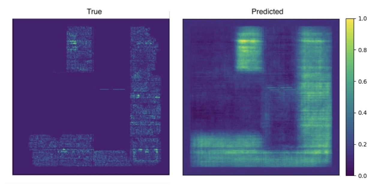
Our Feature Pyramid Network (FPN), as shown in Figure 6, demonstrated progressive improvement as it was trained on the IC chip congestion dataset, highlighting the effectiveness of the architecture in learning hierarchical features. The FPN’s multi-scale feature extraction capabilities allowed it to capture fine-grained and high-level spatial information, essential for accurately predicting congestion regions.

During the initial training epochs, the network showed rapid improvement as it began to learn the fundamental patterns in the dataset. The SSIM loss, which measures the structural similarity between the predicted and ground truth images, steadily decreased, indicating the model’s increasing ability to preserve spatial structures and relationships in its outputs. Simultaneously, the BCE loss, which quantifies pixel-wise classification accuracy, also dropped as the model improved its ability to classify congested versus non-congested regions.

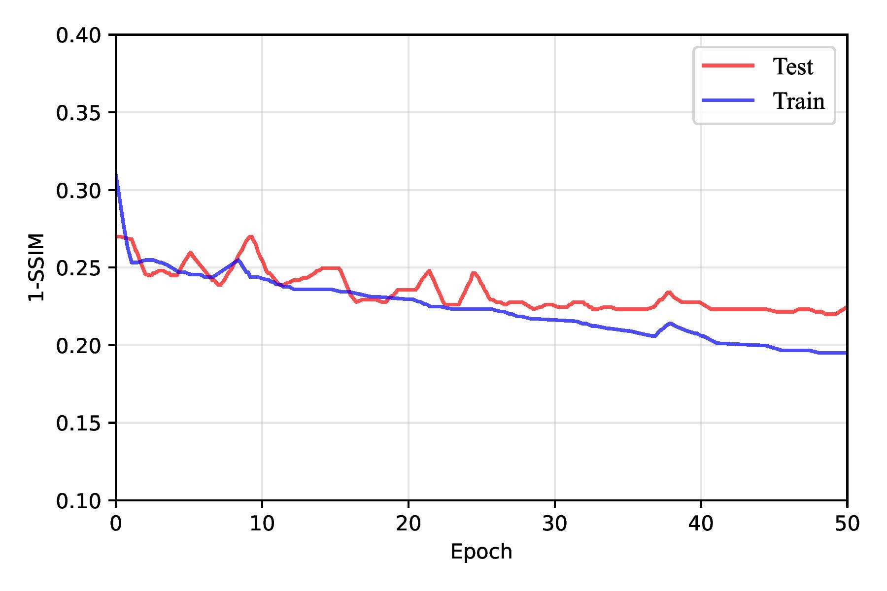
As training progressed beyond the early epochs, the rate of improvement in loss metrics slowed but continued to decline steadily up to around the 30th epoch. However, after approximately 30 epochs, the model began to exhibit signs of overfitting. The training loss continued to decrease, but the test loss plateaued and occasionally increased. This shift suggested that the FPN had started to memorize the training data rather than generalizing it to unseen samples. Overfitting was further reflected in the slight degradation of SSIM and BCE loss metrics on testing data, as shown in Figure 13, emphasizing the importance of implementing strategies such as early stopping, regularization, or data augmentation to mitigate overfitting and enhance generalization. Overall, this training behavior underscored the FPN’s capability to learn progressively while revealing the challenges of balancing model complexity and generalization.

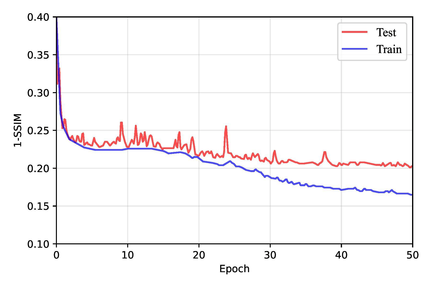
We incorporated dropout as a regularization technique during training to address overfitting in our models and achieve better, more accurate predictions. Dropout works by randomly deactivating a fraction of neurons during each forward pass, which prevents the model from relying too heavily on specific features and forces it to learn more robust and generalized representations. By introducing this randomness, dropout discourages the network from forming overly complex patterns that might fit the training data perfectly but fail to generalize well to unseen data.

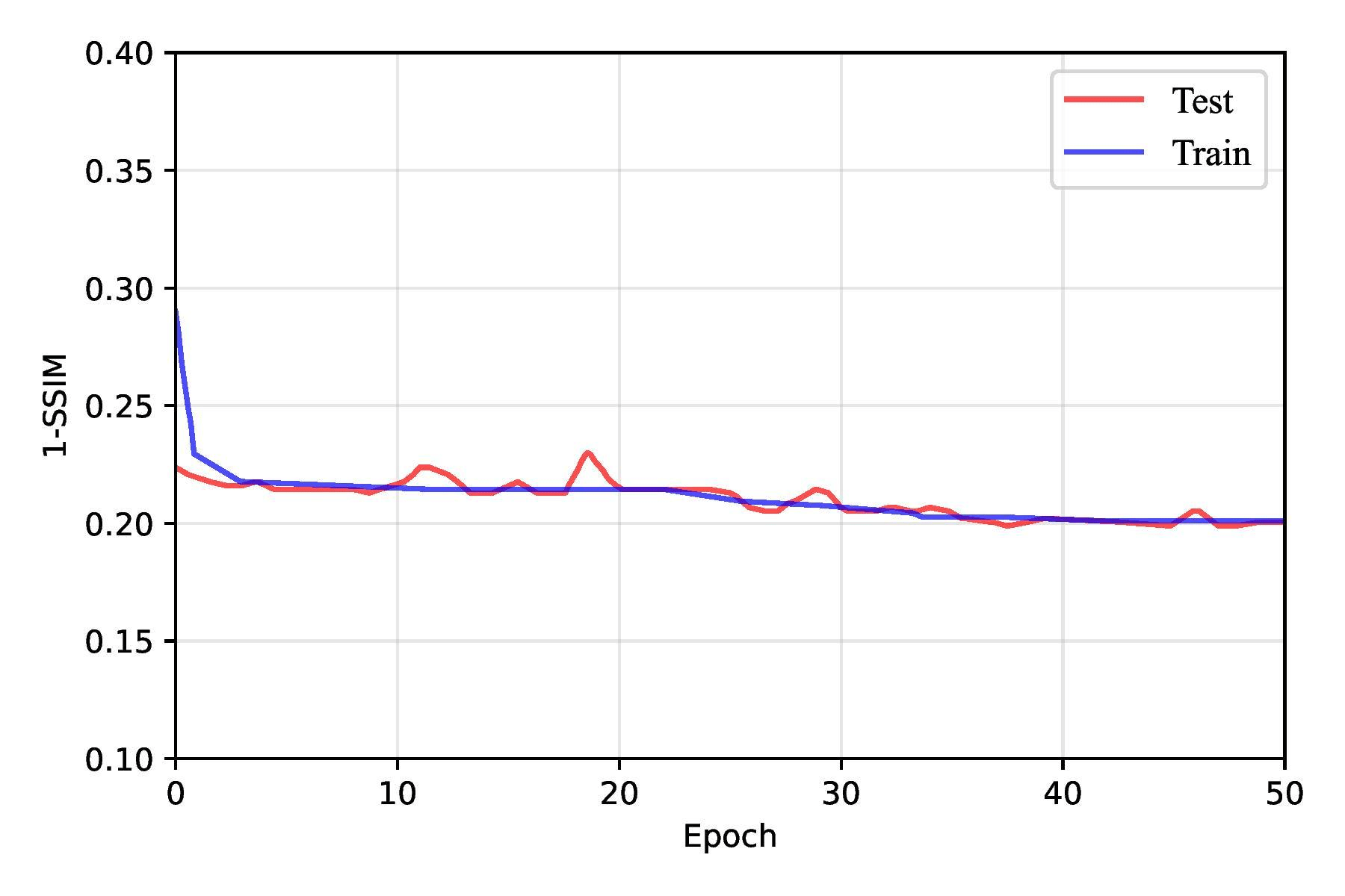
In our implementation, we regularized only the FPN pyramid and left the CNN backbone unchanged. SpatialDropout2D was inserted at the points most prone to overfitting: after the top 1×1 projection; on each lateral 1×1 output; immediately after each top-down fusion add; and after each 3×3 smoothing convolution. Dropout was disabled at evaluation. This single modification improved test 1–SSIM from 0.224 ± 0.017 (no dropout) to 0.199 ± 0.008 as shown in Table 4, Figure 14, and Figure 15. We experimented with different dropout rates, ultimately finding that a rate of 0.0125 struck the best balance between reducing overfitting and maintaining sufficient capacity for learning. During testing, dropout was automatically disabled, allowing the full network to be utilized for making predictions.

Dropout Used?	Test 1–SSIM	Test IoU@τ=90%
No	0.224 ± 0.017	0.52 ± 0.02
Yes	0.199 ± 0.008	0.56 ± 0.02

FPNs excelled due to their ability to integrate multi-scale features effectively. Congestion patterns in IC chips often manifest at different spatial resolutions, from dense, localized hotspots to broader regions of sparse congestion. The FPN architecture is specifically designed to address this by constructing a feature hierarchy that combines low-level details from shallow layers with high-level semantic features from deeper layers. This multi-scale representation allowed the FPN to recognize both small-scale and large-scale congestion patterns with high precision, making it particularly well-suited for the task. While effective in preserving spatial details through skip connections, U-Net lacked the hierarchical feature refinement capabilities of the FPN, which limited its performance on datasets with complex, multi-scale features.

Performance derives from explicit multi-scale fusion. Lateral 1×1 projections preserve high-level semantics from deeper stages, the top-down pathway transports context to finer resolutions, and the smoothing convolutions restore edges after fusion. This sequence keeps narrow routing channels at macro boundaries intact while still following broad RUDY-driven gradients. The model handles cases where congestion depends simultaneously on fine macro geometry and wide-area demand, which is where encoder–decoder baselines and patch-token models give ground.

Error Analysis

The FPNs worst errors are concentrated in three problems. First, diffuse congestion is under-estimated when demand rises broadly without strong edges. The FPN is able to find localized regions and hotspots but tends to underestimate broad congestion across a floorplan. Second, the model has a tendency to smooth out narrow choke points at the boundaries of macro regions. The top-down pyramid loses some information here. Finally, periphery zones show mild false positives because boundary context is missing. All of these errors result in small SSIM penalties of around 0.01, but they are areas for future work to address nonetheless.

When broken down by chip type, the FPN has some limited bias. CPU-style floorplans perform slightly better than the aggregate, but array-heavy GPU blocks degrade SSIM by about 0.007 and accelerator designs with long global interconnects degrade SSIM by 0.01. This is caused by long-range coupling being blurred by bilinear upsampling in the pyramid. Residual heatmaps localize these errors to macro corners, thin channels, and die edges; the effect does not overturn the overall ranking but marks the limits of multi-scale fusion without additional inputs.

Overall, FPNs and Vision Transformers outperformed U-Net and autoencoders by leveraging their advanced mechanisms for multi-scale feature integration and global contextual understanding, respectively. These capabilities were crucial for handling the complex and hierarchical congestion patterns in IC chips, where simpler architectures like U-Net and autoencoders fell short.

These models can be generalized to other datasets. Due to the size of our dataset (10000+ samples) and a range of data augmentation techniques, our models can capture underlying spatial patterns in congestion. As a result, our approach is not only effective for our dataset but is also well-suited for generalization to other IC congestion datasets with similar structural characteristics.

Ablation Study Results

We performed an ablation study focused on input features used by FPN as shown in Table 5. The same dataset splits, parameters, and metrics were used. RUDY is the dominant signal. Using RUDY alone outperforms Macro-only and RUDY_PIN-only by a wide margin. Adding Macro to RUDY lifts structure and overlap. The gain stems from capacity awareness: macro masks suppress false positives in corridors with limited routing resources and along the periphery where keep-outs and PDN effects alter usable tracks. Adding RUDY_PIN to RUDY also helps by sharpening peaks at macro corners and pin-dense edges, which reduces narrow-channel misses.

All three features together perform best. The improvement over the two-feature variants is smaller but consistent, reflecting complementary roles: RUDY provides broad demand, Macro encodes coarse blockages and capacity, and RUDY_PIN refines local routing pressure near pin clusters. RUDY is overall the best input, with Macro Regions augmenting global congestion patterns and RUDY_PIN highlighting sharper edges and structures in smaller regions.

Inputs used	Test 1–SSIM	Test IoU@τ=90%
Macro + RUDY + RUDY_PIN	0.199 ± 0.008	0.56 ± 0.02
RUDY + RUDY_PIN	0.206 ± 0.010	0.54 ± 0.02
Macro + RUDY	0.212 ± 0.008	0.53 ± 0.02
Macro + RUDY_PIN	0.248 ± 0.011	0.48 ± 0.02
RUDY only	0.258 ± 0.009	0.45 ± 0.02
RUDY_PIN only	0.301 ± 0.013	0.38 ± 0.03
Macro only	0.322 ± 0.014	0.35 ± 0.03

Real World Applicability

Easing routing congestion benefits key Power Per Area (PPA) metrics and improves chip design in a few ways. Placement strategies that minimize congestion are known to reduce signal delays, thereby improving timing slack¹⁹. In industry practice, congestion-aware placement yields better worst negative slack (WNS) and total negative slack (TNS) along with lower power consumption²⁰, linking routability improvements to final performance. While we acknowledge that surrogate metrics sometimes misalign with final PPA, our approach targets congestion specifically because it underlies many timing violations and excess power (via long interconnects and detours). By predicting and mitigating congestion hotspots early, we enable subsequent optimization stages (timing closure, buffering, etc.) to achieve better WNS/TNS, fewer violating paths, and area/power benefits than would be possible on a highly congested layout.

Another advantage of our models is reducing coupling capacitance crosstalk. In the past, studies have shown that crosstalk noise hotspots often do not perfectly overlap with routing overflow hotspots, so congestion alone is an imperfect proxy for signal integrity. While our models do not directly evaluate crosstalk noise, by reducing severe congestion, the placement is likely to have fewer tightly-packed parallel nets, which can indirectly mitigate some coupling issues and thus improve signal integrity (less aggressive crosstalk)¹⁹.

Limitations and Scope

Congestion minimization is not a silver bullet for timing closure or power issues under all conditions, especially at activity extremes. We nevertheless chose congestion as our focus because it significantly impacts downstream timing and power. Dense routing congestion forces longer wire detours and more buffering, which degrade timing and raise dynamic power, so alleviating congestion can directly reduce these effects¹⁹. However, extreme scenarios (e.g., worst-case simultaneous switching or traffic bursts) demand additional measures beyond congestion reduction – such as robust clock distribution, dynamic voltage drop mitigation, and multi-corner timing optimization – to fully close timing and manage power. Our approach addresses one fundamental aspect (routability), ensuring that timing closure tools have a cleaner canvas to work with once congestion is reduced. This is meant to complement, not replace, other PPA optimization steps. Minimizing congestion helps enable timing closure and lowers power via shorter interconnects, but it must be combined with other techniques to handle the worst-case scenarios²¹. Timing closure and power dissipation at traffic flow extremes are potential avenues for future research.

Our work is limited to 2D classical computing chips. Quantum computing chips involve very different design paradigms (e.g. superconducting qubit layouts and cryogenic control circuits), meaning classical physical congestion metrics do not directly apply²². Thus, our current approach would not generalize to such chips without significant modification. Likewise, 3D integrated circuits introduce a vertical dimension of routing (through-silicon vias and cross-tier interconnects) that alters congestion patterns. Extending our models to 3D chips would require new feature engineering (such as per-tier RUDY maps or via-density metrics) and retraining on 3D design data.

NoC (On-Chip Network) congestion is another category our research does not cover. In a NoC, congestion occurs at the network level (buffer queues and packet latency) rather than as physical wiring overflow, and it behaves differently from conventional wire congestion²³. For example, in a bufferless NoC design, congestion can throttle packet injection and reduce system throughput depending on application traffic patterns, which necessitates an application-aware throttling strategy²³. Our work focuses on physical layout routability – predicting regions where wiring demand exceeds capacity on the chip layout. Our model identifies placement regions likely to suffer routing congestion (high routing demand), not runtime traffic congestion in a network fabric. A similar learning framework could be extended with NoC-specific features (e.g., link utilization or buffer occupancy metrics) to predict network congestion in the future.

To sum, the focus of our research was on reducing congestion on 2D classical computing chips using machine learning models. Our models performed well for this purpose, and future research has multiple potential avenues to explore, including optimizing for other metrics or focusing on different types of chips.

Conclusion

This study resolves a practical gap: early-stage congestion prediction lacked an apples-to-apples comparison of modern architectures under a single dataset, input, and metric regime. We created a standard protocol (CircuitNet; Macro, RUDY, RUDY_PIN; structure-aware similarity) and quantified uncertainty with bootstrap resampling, isolating architectural effects.

Two methodological choices matter. First, architecture families with hierarchical or global context win: FPN delivers the lowest 1–SSIM of 0.199 ± 0.008, with ViT close behind at 0.223 ± 0.011, confirming that multi-scale and self-attention can model congestion more effectively than simple encoder–decoders. These models beat the UNet baseline of 0.342 ± 0.010 and prior work, which achieved a 1-SSIM of 0.336. Second, targeted regularization can prevent overfitting. Pyramid-only SpatialDropout2D (p≈0.0125) reduces overfitting in the fusion path, allowing the model to balance learning and generalizing.

For evaluation metrics, SSIM is clearly the superior choice for comparing congestion maps. BCE-with-logits outperforms MSE as a loss function by preserving the edges and contrast that SSIM rewards. Complementary metrics like IoU align with the SSIM ranking, indicating consistent gains. The FPN achieved an IoU score of 0.56 ± 0.02, and the ViT was not too far behind at 0.51 ± 0.02.

An ablation study with the FPN isolated feature contribution. Using RUDY alone yields 1–SSIM ≈ 0.238 and IoU ≈ 0.49. Adding Macro Regions improves capacity awareness (Macro+RUDY ≈ 0.212, IoU ≈ 0.53). Adding RUDY_PIN to RUDY sharpens peaks near pin-dense regions (RUDY+RUDY_PIN ≈ 0.206, IoU ≈ 0.54). To sum, RUDY is the dominant signal; Macro reduces false positives in low-capacity corridors and at the periphery; RUDY_PIN refines local hotspots at macro boundaries.

Industry implications are direct. Using these predictors as early screeners during floorplanning and initial placement can eliminate high congestion maps early in the design process. Overall, our models can lead to improved WNS/TNS through shorter detours, improved coupling capacitance, and lower dynamic power from reduced wirelength.

The potential for future research is high. Avenues to be explored include stress-test cross-design transfer, domain-generalization and calibration layers for new PDKs, congestion prediction with timing and power co-targets in a multi-task head, and lightweight netlist proxies that preserve early-stage deployability. This paper is a usable recipe of data, evaluation metrics, and models to create an early warning signal to streamline computer chip production.

References

1. H. Jiang, L. Qing, J. Yong, S. Gengbiao, S. Richard, T. Chen, M. Xu.  When machine learning meets congestion control: A survey and comparison. Computer Networks. 192, 108033, (2021). [↩]
2. J. Westra, C. Bartels, P. Groeneveld. Probabilistic Congestion Prediction. Association for Computing Machinery.  204–209, (2004). [↩]
3. Z. Xie, Y.-H. Huang, G.-Q. Fang, H. Ren, S.-Y. Fang, Y. Chen. RouteNet: Routability Prediction for Mixed-Size Designs Using Convolutional Neural Network. Proceedings of the ACM/IEEE International Conference on Computer-Aided Design (ICCAD). 80, 1-8, (2018). [↩] [↩]
4. S. Zheng, L. Zou, P. Xu, S. Liu, B. Yu, M. D. F. Wong. Lay-Net: Grafting Netlist Knowledge on Layout-Based Congestion Prediction. Proceedings of the IEEE/ACM International Conference on Computer-Aided Design (ICCAD). 1-9, (2023). [↩] [↩]
5. H. Li, Y. Huo, Y. Wang, X. Yang, M. Hao and X. Wang. A Lightweight Inception Boosted U-Net Neural Network for Routability Prediction. 2024 2nd International Symposium of Electronics Design Automation (ISEDA). 648-653, (2024). [↩] [↩] [↩]
6. B. Wang, G. Shen, D. Li, J. Hao, W. Liu, Y. Huang, H. Wu, Y. Lin, G. Chen, P. A. Heng. LHNN: Lattice Hypergraph Neural Network for VLSI Congestion Prediction. Proceedings of the 59th ACM/IEEE Design Automation Conference (DAC). 1297-1302 (2022). [↩]
7. Z. Chai, Y. Zhao, W. Liu, Y. Lin, R. Wang and R. Huang, “CircuitNet: An Open-Source Dataset for Machine Learning in VLSI CAD Applications With Improved Domain-Specific Evaluation Metric and Learning Strategies,”. IEEE Transactions on Computer-Aided Design of Integrated Circuits and Systems. 42 (12), 5034-5047, (2023). [↩]
8. A. Dertat. Applied Deep Learning – Part 3: Autoencoders. Medium. (2024). [↩]
9. Y. Li, Y. Li, X. Zhu, H. Fang, L. Ye. A method for extracting buildings from remote sensing images based on 3DJA-UNet3+. Scientific Reports, 14, 19067. (2024). [↩]
10. U-Net architecture Y. Ding, F. Chen, Y. Zhao, Z. Wu, C. Zhang, D. Wu. A Stacked Multi-Connection Simple Reducing Net for Brain Tumor Segmentation. IEEE Access. 7, 104011-104024. (2019). [↩]
11. A. Dosovitskiy, L. Beyer, A. Kolesnikov, D. Weissenborn,  X. Zhai, T. Unterthiner, M. Dehghani, M. Minderer, G. Heigold, S. Gelly, J. Uszkoreit, N. Houlsby. An image is worth 16×16 words: Transformers for image recognition at scale. Verbal ICLR. (2021). [↩] [↩]
12. M. Tan, R. Pang and Q.V. Le. EfficientDet: Scalable and Efficient Object Detection. 2020 IEEE/CVF Conference on Computer Vision and Pattern Recognition (CVPR). 10778-10787 (2020). [↩]
13. L. Tsung-Yi, P. Dollar, R. Girshick, K. He, B. Hariharan, S. Belongie. Feature Pyramid Networks for Object Detection. IEEE Conference on Computer Vision and Pattern Recognition (CVPR). 936, 44, (2017). [↩]
14. X. Xu, D. Z. Pan. Toward Unidirectional Routing Closure in Advanced Technology Nodes. IPSJ Transactions on System LSI Design Methodology. 10, 2–12, (2017). [↩]
15. Z. Wang, A.C. Bovik, H.R. Sheik, E.P. Simoncelli. Image Quality Assessment: From Error Visibility to Structural Similarity. IEEE Transactions on Image Processing 13. 4, 600–612, (2004). [↩] [↩]
16. S. Jadon. A survey of loss functions for semantic segmentation. 2020 IEEE Conference on Computational Intelligence in Bioinformatics and Computational Biology (CIBCB). 1-7, (2020). [↩]
17. S.A. Hussain, S. Karimulla, F. Shaik, S.B. Javeed. Deep Learning-Based Congestion Control in VLSI for Placement and Routing. Journal of Theoretical and Applied Information Technology. 102 (24), (2024). [↩]
18. A. Mirhoseini, A. Goldie, M. Yazgan, J.W. Jiang, E. Songhori, S. Wang, Y.J. Lee, E. Johnson, O. Pathak, A. Nova, J. Pak, A. Tong, K. Srinivasa, W. Hang, E. Tuncer, Q.V. Le, J. Laudon, R. Ho, R. Carpenter, J. Dean. A graph placement methodology for fast chip design. Nature. 594, 207–212 (2021). [↩]
19. N. Gurushankar. Importance of Timing Closure in Semiconductor Verification. International Journal For Multidisciplinary Research. 6 (6), (2024). [↩] [↩] [↩]
20. M. Saeedi, M.S. Zamani, A. Jahanian. Evaluation, Prediction and Reduction of Routing Congestion. Microelectronics Journal. 38 (8-9), 942-958, (2007). [↩]
21. J. Hu, K. Andrew. Invited Paper: The Inevitability of AI Infusion Into Design Closure and Signoff. USCD Invited Paper. (2024). [↩]
22. B. Zhao, Z. Li, X. Yu, B. Yuan, C. Zhang, Y. Gao, W. Wang, Q. Mu, S. Wang, H. Sun, T. Yang, M. Zhang, C. Han, P. Xu, W. Wang, Z. Shan. EDA-Q: Electronic Design Automation for Superconducting Quantum Chip. IEEE Transactions on Computer-Aided Design of Integrated Circuits and Systems. 99, 1, (2025). [↩]
23. G. Nychis, C. Fallin, T. Moscibroda, O. Mutlu, S. Seshan. On-Chip Networks from a Networking Perspective: Congestion and Scalability in Many-Core Interconnects. Association for Computing Machinery. 42(4), 407-418, (2012). [↩]