Maximizing Bank Telemarketing Effectiveness Through Machine Learning and Data Balancing Techniques

Abstract

This study was conducted with the goals of improving the success rate of telemarketing outcomes by using model prediction to determine the success rates of telemarketing campaigns. This would be done by using random forest, XGBoost, and neural networks to both find the best model in predicting the success rates and determine which variables were most impactful in model prediction. The dataset that was used was heavily imbalanced towards failures in telemarketing outcomes, so numerous imbalancing techniques were used, including class weighing, SMOTE, undersampling, and a mixture of the last two. In order to determine which model paired with which data balancing strategy was the most effective, we used the metrics of precision, recall, and f1 scores over accuracy. We felt that this gave the overall most effective model as with accuracy, one of the outcome’s scores could heavily inflate the accuracy, making the model seem better than it actually was. The experiment resulted in undersampling yielding constantly the best results with the best model being XGBoost with a f1 score of 0.87 and 0.88 for outcomes of 0 and 1, respectively. More advanced models such as neural networks didn’t achieve greater results than the one given by XGBoost. Additionally, in order to find which variable was most impactful on model prediction, we used SHAP values which resulted in duration having the greatest SHAP value, followed by emp.var.rate, nr.employed, eribor3m, and cons.conf.idx (a higher SHAP value correlates to greater importance on model prediction). This finding led us to have our best model, the undersampled XGBoost, to use the dataset with only the values of the variables with the top SHAP values, giving us a f1-score of 0.87 and 0.88 for outcomes of 0 and 1, respectively. This showed that the variables with the highest SHAP value are most important and telling in model prediction.

Keywords: telemarketing, machine learning, data imbalance, SMOTE, undersampling, class weights, shap analysis

Introduction

Telemarketing campaigns are one of the most popular ways for companies to try and gain new customers, however they are relatively ineffective. With so much money going into this style of marketing and an average of 2.35% conversion rate¹, actions must be taken in order for companies to not waste so much money every year. In order for people to improve the marketing outcomes of telemarketing campaigns, the most impactful characteristics that affect the success rate of the campaign must be found². Understanding the contribution of various factors on the outcomes of telemarketing is a crucial step for companies to identify individuals who most likely say yes to their campaign. This allows for companies to take action and change their marketing strategies to follow the trends in the data. Without this step, marketing strategies won’t be as fruitful in attracting new or returning customers.

Telemarketing is especially important to banks as it is one of their largest methods of gaining and maintaining customers. Just in 2023, the telemarketing market was $12.6 billion and is expected to grow to as much as $15.5 billion by 2030³. If banks are able to target individuals during telemarketing campaigns, banks would be able to use these billions of dollars more effectively than ever.

With the appropriate marketing strategies, banks are able to target which aspects or factors are the most influential in whether or not the telemarketing campaign will work. They can also use data driven models that are proven to be effective in predicting whether or not the campaign will work. This allows banks to better optimize customer targeting for the highest rates of success, along with potentially predicting which customers have the highest potential in subscribing to their services. With the advances in machine learning, it would be faster and much more efficient to identify the campaigns that will most likely succeed, and to understand what factors are the most or least vital in predicting campaign success.

Moro et al.,⁴ proposed a data-driven approach to predict the success of bank telemarketing. They utilized four machine learning models such as: logistic regression, decision trees, neural networks, and support vector machines. They determined the highest accuracy through 2 different metrics: area of the receiver operating characteristics curve (AUC) and the area of the LIFT cumulative curve ALIFT). Neural Networks ended up presenting the best results with AUC yielding a 0.8 and ALIFT yielding 0.7. These scores however, might not be the most accurate due to the fact that only 1293 contacts were used in the testing data, out of a total of 52944 contacts. With just under 2.5% of the data available being used in the testing data, it makes us wonder whether the results are as accurate as possible, or if with more references in the testing data, the results would’ve been lower. Additionally, there were no data balancing techniques used in the study even though they also mentioned how the data was imbalanced, furthering our belief that the results aren’t fully correct.

Ilham et al.,⁴ conducted a comparative study of various classification models to predict the success of bank telemarketing. They used seven different models being Decision Tree (DT), NaïveBayes (NB), Random Forest (RF), K-Nearest Neighbour (K-NN), Support Vector Machine(SVM), Neural Network (NN), and the Logistic Regression (LR) model. They used area under curve (AUC) and accuracy to rate how well each model predicts the results. In the end, the SVM had a 0.925 score on the AUC. The main limitation of this study is the use of the accuracy score as it can be misleading due to the data imbalance.

Bogireddy et al.,⁵ used the evaluation metrics of precision, recall, f1-score, and accuracy. They used the models of XGBoost, Gradient Boosting, Logistic Regression, Decision Tree, and K-Nearest Neighbors. XGBoost ended up being the best model yielding an f1-score of 0.85 and 0.84 for outcomes of 0 and 1 respectively, with an overall accuracy of 0.84. They only used SMOTE however in their data balancing techniques, leading to a factor they missed being to try other methods such as undersampling. Another key factor this study missed is the feature importance analysis to understand the contribution of different factors on model predictions.

Peter et al.,⁶ used the metrics of accuracy and ROC-AUC (Receiver Operating Characteristic – Area Under the Curve). The models used were Random Forest, Bagging Classifier, Boosting Model, Gradient Boosting, AdaBoost, Stacking Model, and Stacking with Gradient Boosting yielding the highest values of 0.9185 and 0.9476 for accuracy and ROC-AUC respectively. While these scores might seem high, the f1-score of their model is 0.5951 which is quite low. Accuracy can be deceiving due to the imbalanced dataset, leading the results to not be quite accurate. We also question how accurate these scores are as since accuracy is a combination of f1-scores, a low f1-score should result in a similarly low accuracy however in their results, there seems to be no correlation between the two values at all.

These prior published studies have all created machine learning models that predict the outcomes of telemarketing campaigns and have found the best ones. The main limitations seen in these studies are that some machine learning models are not used/tested in prediction, the evaluation metrics used are accuracy or another form of this, which can be heavily skewed due to the imbalance dataset, and that they fail to use any data balancing techniques in their tests. Another missing part of most of the studies is the feature impotence analysis where they don’t find the most impactful variables on model prediction, not allowing for greater understanding of the features and the overall topic.

Having a reliable machine learning model that is able to precisely predict consumer conversion rates in telemarketing campaigns will save companies a significant amount of advertising funds. If the model were to give a false positive, then money and time would be lost trying to win over a customer who already had a low conversion chance. A false negative leads to not using any resources, however losing a potentially crucial customer for the future.

The objectives of our study are (1) develop a highly reliable machine learning model that performs well in predicting outcomes of telemarketing, (2) systematically investigate and mitigate the data imbalance issues, (3) quantify and rank the contribution of various factors related to bank client, product and social-economic attributes on model predictions.

Dataset

In this study we used a dataset about a marketing campaign from a Portuguese banking institution that was based on telemarketing⁷. In total our dataset contains 45,211 individuals surveyed during the campaign. Additionally, there were 21 different columns, or variables, that differed between each person as shown in Table 1.

The most basic columns were the age of the individuals surveyed, their job and marital status, highest level of education completed, and whether the client had a personal loan. Another group of variables describes the information about the contact of the consumer. This includes the contact method, the month, day of the week, and duration of the call. The dataset additionally included information about terms before and after the contact. This covers the number of contacts with the client before the campaign, the number of days since the client was contacted last, the number of contacts performed before the campaign, and the outcome of the previous marketing campaign for the client. Finally, we used an updated version of the dataset that added information about the employment variation rate, consumer price index, consumer confidence index, 3 month rate daily indicator, and the number of employees of the company. We dropped the variable called default, meaning whether or not the client has credit on a default, because all the individuals had not defaulted in our dataset. This took us from 41,188 data points to 31,828. Additionally, we dropped deleted some data from our dataset in which the housing column was unknown, setting our Our target is a binary column that indicates whether the client has subscribed for a term deposit.

Table 1. Input and output variables description

Variable Name	Type	Description
age	Numeric	Age of the client
job	Categorical	Client’s occupation
marital	Categorical	Marital status
education	Categorical	Client’s education level
default	Categorical	Indicates whether the client has credit in default
housing	Categorical	Indicates whether the client has a housing loan
loan	Categorical	Indicates whether the client has a personal loan
contact	Categorical	Type of contact communication
month	Categorical	Month that last contact was made
day_of_week	Categorical	Day that last contact was made
duration	Numeric	Duration of last contact in seconds
campaign	Numeric	Number of contacts performed during the campaign for the client
pdays	Numeric	Number of days since the client was contacted in a previous campaign
previous	Numeric	Number of contacts performed before this campaign for this client
poutcome	Categorical	Outcome of the previous marketing campaign
empvarrate	Numeric	Employment variation rate
conspriceidx	Numeric	Consumer price index
consconfidx	Numeric	Consumer confidence index
euribor3m	Numeric	Euribor 3-month rate
nremployed	Numeric	Number of employees
outcome	Binary	Whether the client has subscribed for a term deposit

Exploratory Data Analysis

By comparing different variables with each other and finding the correlations between them, we were able to get a better understanding of the relationship between the variables. We compared them through different graphs and plots. Through these exploratory studies, different patterns and correlations emerged which will be described below along with the graphs.

Figure 1 illustrates the count distribution of a successful (yes) or failed (no) telemarketing outcome. The failures have over 27,727 representations in the dataset while the successes had 4,101. The substantial difference in the count between them demonstrates how the data is greatly imbalanced toward the failure side.

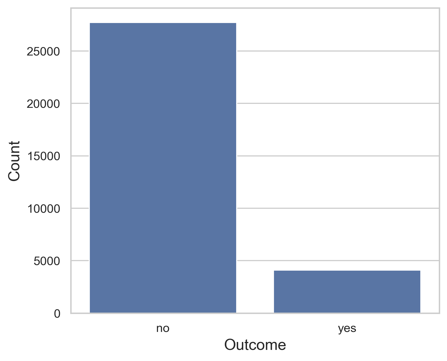
Figure 2 shows the heat map of the correlation between variables. The squares that are dark blue represent a significant correlation between the variables that it represents while a dark red signifies a strong negative correlation. The lighter squares represent a lack of correlation between the variables it represents. When looking at the data, we can see that there is a significant correlation between emp.var.rate and euribor3m with a score of 0.97. This shows that the data in each variable is extremely similar, allowing us to potentially remove one or the other while keeping similar results in the model due to how interchangeable they are. The correlated pairs with a score of above 0.8 as shown by this were emp.var.rate and euribor3m with a score of 0.969, emp.var.rate and nr.employed with 0.899, and euribro3m with nr.employed with a score of 0.944.

Figure 3 demonstrates the outcomes on the x-axis to the duration on the y-axis. This allows us to get a better understanding of how the two correlate as we can see durations with the highest chance of success, along with the highest chance of failure. We can see this as the blue box represents the greatest concentration of values for the duration and the box for the successful campaign being greater than the failing campaign shows how with a higher duration, there is a greater likelihood that the consumer will buy the product.

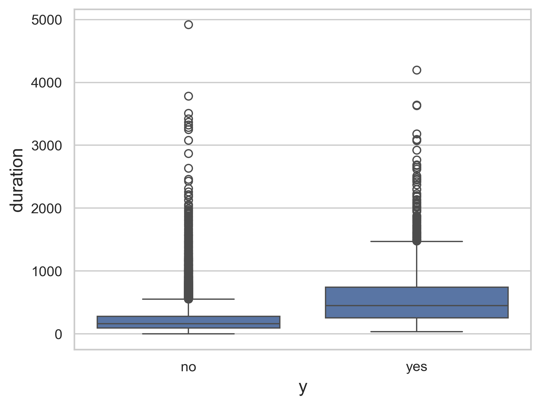
Figure 4 below is another box plot that shows the greatest concentrations of the employment variation rate in terms of which ones succeeded and which failed. The successes have a significantly clearer range of around 0 to -2 while the failures are much more spread out with 1.5 to -2. Using this knowledge, we can determine that the highest values of the emp.var.rate feature will result in a failure while lower values at around -1 on average will result in the best chance of a successful campaign.

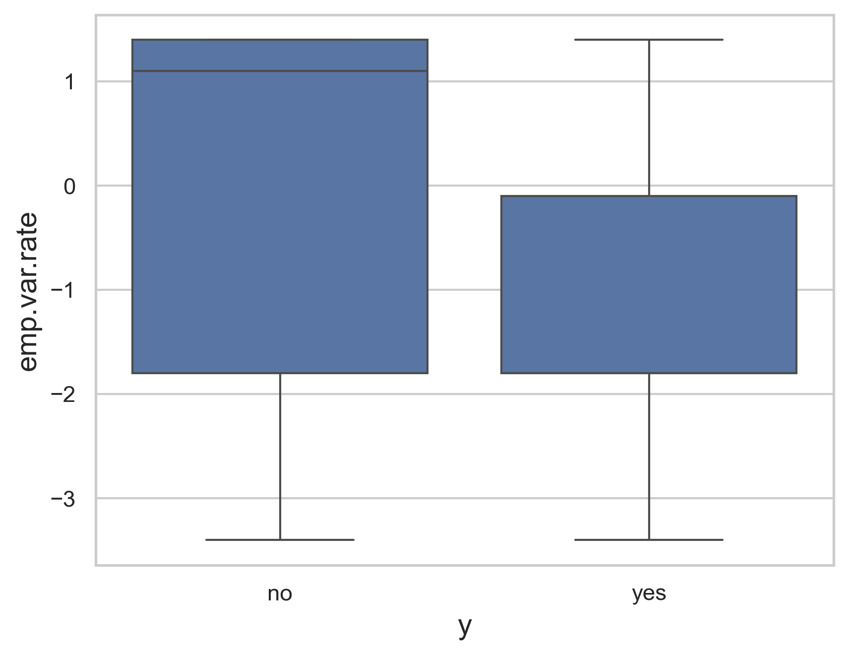
Figure 5 demonstrates the relationship between nr.employed with the outcome. The successes have a very broad range of around 5180 to 5025, while the failures are much more concentrated around 5225 to 5100. From this, we can tell that any value of nr.employed that is greater than 5180 while have a significantly greater chance of failing rather than succeeding, whereas numbers between 5100 and 5025 while have a higher chance of succeeding. Between the values of 5180 and 5100 however, there isn’t a clear outcome with both outcomes having a decent chance of occurring.

Figure 6 demonstrates each of the containers within outcome being nonexistent, failures, or success and their counts, while also being sorted by if they succeeded or not. Poutcome is the variable signifying if there has been a previous campaign attached to the customer and if there is, whether it succeeded or failed. It appears that there aren’t many customers who did get reached out to prior to this exchange, however of the ones that did, most times it had succeeded, it succeeded here whereas if it had failed before, it usually failed again.

Figure 7 demonstrates the relationship between the contact method and the outcomes. In this, it can be seen that cellular devices were used significantly more, but also seemed to have a better ratio in successes to failures than did telephones. The cellular devices had around a 1:5 ratio while the telephones had around a 1:15 ratio. This showed that using cellular devices is usually the better contact method when telemarketing than contacting telephones.

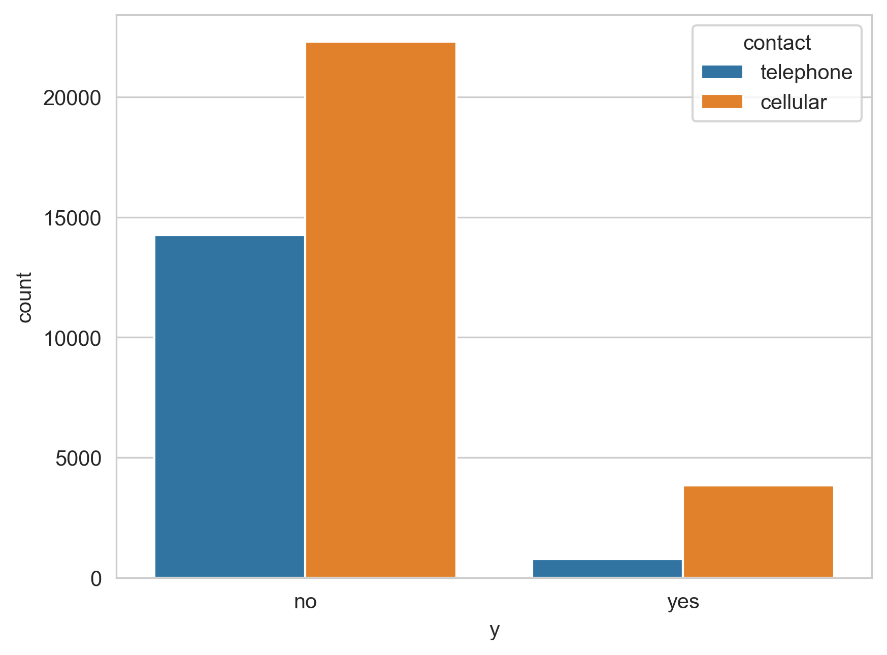
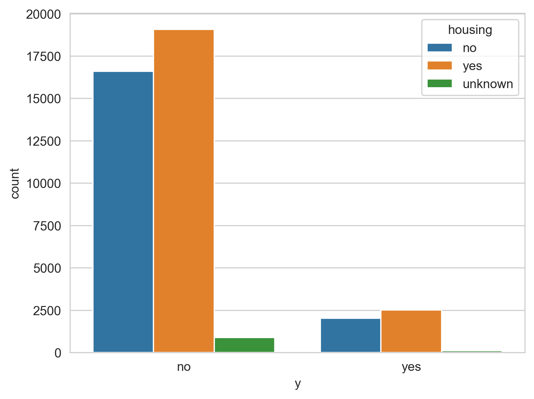
Figure 8 is the representation of the housing column compared to the y (outcome) column. In this it is shown that there is a mostly even split between those with housing loans and those without. The ratio between the ones with loans who said yes to the campaign compared to the ones that didn’t is around 1:7.5 while the ones without loans ratio is around 1:7. This shows that with mostly even numbers, individuals without housing loans are slightly more likely to agree with the campaign than are those who are housed.

Methods and Models

Data Preprocessing

Standard scaling was used on the variables that are either an integer or a float. This type of scaling shifts each of the values to have a median of zero and a standard deviation of one. This allows it to keep the relationship between the data points to be equal to what it was before, while also shrinking the values. When the values shrink, the bias of larger values is greatly decreased as all values are between zero to one, resulting in the ranges of all integer and float values to be the same. Without scaling the numeric data, values that initially had a significantly larger range than others would’ve been held at a higher regard than those with smaller ranges. Standard Scaling was used on all columns with an integer or float data type. This includes age, duration, campaign, pdays, and previous for integers, and emp.var.rate, cons.price.idx, cons.conf.idx, euribor3m, and nr.employed for floats.

A few variables from the data from the dataset also went through data cleaning or data grouping. This involves replacing some of the values within each variable with others in order to lessen the number of values or remove unknowns from a column. The variables of job, education, and marital were subjected to both of these processes. The different responses in the job column were put into employed, or unemployed depending on if they had jobs or not. Education had three categories: uneducated which included middle school and below or no education at all, med-education which included mainly the group with a high school diploma, and high education which had a university degree or a professional course finished. Finally, marital was just made into 2 categories of either married or single.

One of the encoding techniques used was ordinal encoding, and was also used on three different variables. Ordinal encoding is used to make the machine learning model hold one response in a higher regard than another. This is done by assigning numerical values to each literary value from a variable. In most cases, the values are assigned in ascending order in terms of each variable’s inherent or natural order. The variables that were ordinal encoded were job, education, and poutcome. For job, employed was given a value of 1 while unemployed was given 0. Education had the high education value as 2, medium education as 1, and no education as 0. Finally, poutcome had success put as 2, failure as 1, and nonexistent as 0.

The other encoding technique used was one hot encoding. One hot encoding is done by splitting one variable into multiple with regards to each unique value of the variable. The new variables are then either booleans or integers with a value of 1 or 0 (1 being true 0 being false). This allows for both no order bias in the models, while also making it somewhat easier to see the connections between the variable values and the outcomes. It also provides a greater understanding of how the day of the week, for example, impacts the success of the campaign and which days of the week are the most influential on the outcome, if any. The variables that were impacted by this encoding technique were contact, month, and day_of_week.

Handling an Imbalanced Dataset

This dataset is challenging because the ratio of failures to successes outcomes is incredibly unequal, also known as an imbalance dataset. The ratio is around 27,000 for failures to 4,000 successes. This colossal data imbalance may result in the models heavily favoring failures when predicting the outcomes of a campaign. We offset this by evaluating four different methods: balancing the class weights in the algorithm, undersampling, oversampling (SMOTE), and a mix of the last two techniques.

When we balance the class weights, we take the outcome with less occurrences, in this case the successes, and make them weigh more to the algorithm than the majority class. This makes it so that each success will have a greater impact on the overall system, reducing the bias towards failures.

Undersampling is when the value with a greater amount is brought down to the same as the amount of the smaller value. In this case, the failures would be shrunk down to 4,101 to match the amount that succeeded. This allows for a more balanced dataset with all the original points, however also has the result of decreasing lots of information from the original dataset.

Oversampling, also known as SMOTE⁸, involves creating synthetic data in order to again, even out the data imbalance. This is done by using the existing data points and creating new synthetic data between existing ones. This effectively increases the diversity of the minority class, while also not completely contaminating the data with false information. This again balances the dataset and allows the models to more accurately predict the outcomes of the telemarketing campaigns. Oversampling techniques are applied to training data only.

The final method of combining the two is done by first undersampling the original data, then splitting the undersampled data into a train and a test set, and then using SMOTE only on the training data⁹. While SMOTE doesn’t feed the models completely false data, it also isn’t completely pure as there is no account of it happening genuinely in the dataset. It being after the splitting of the data allows for the complete purity of the data used to test the accuracy of the models, allowing for completely accurate test results. In this, we first undersampled the failures to around 50% of what it originally was, from 27,727 to 13,863. Then we split the data into train and test and finally used SMOTE on the train dataset.

Models and Evaluation Metrics

Before using the models, we split the data into two different parts, train and test, using stratify split. The train data is used to help train the model and is made up out of a random 70% of the telemarketing outcomes. Test data is what the model is tested on. It is a portion of the dataset that the model has never seen before and the results are seen as how well the model performs. It is made up of the remaining 30%.

We implemented two ensembled based models, such as random forest, and XGBoost, and neural networks. The first method that was tried in this study was random forest¹⁰. This machine learning model integrates several decision trees, with each tree being given and trained on a random portion of the dataset from the training data which was given to the model. The tree is made up of internal nodes which it gives the information which keeps splitting until it reaches the final nodes called leaf nodes. Finally, the decision tree then chooses an outcome for a situation from a new set of data, the testing data, based on what they had been trained on from the training data and what the leaf nodes say when the new data is passed through the tree. The ultimate predicted outcome of the situation from the testing data is then decided by whichever the majority of decision trees decides. This allows for a minimized likelihood of overfitting and gives a decent ending accuracy.

Another model that was used was XGBoost¹¹. It stands for extreme gradient boosting and is a machine learning algorithm that also predicts using decision trees, however it uses them in a different way. It stacks multiple decision trees on top of each other, allowing each to learn from its successor’s mistakes. It uses regularization to prevent the overfitting of the data and ensures the model responds well to unseen and new data. It is significantly faster than random forest as it doesn’t use as many decision trees, but is still quite accurate.

The final model used is neural networks¹². This works by using interconnected nodes, called neurons, which are organized by the layers they are in. Each neuron will receive an input from another neuron and process it using one method. The output of each neuron is passed to the next layer, in which the model learns by adjusting the weights between neurons, based on the data. This process allows the network to make predictions through patterns it identifies.

In order to better understand which values of the parameters ended up providing the best results in model prediction, we used the evaluation metrics of precision, recall, f1-score, and area under the curve (AUC). Precision is the percentage of the predictions that came out as positive, which are in reality, also positive¹³. Recall score measures out of all the true positive outcomes, which ones did the model predict were positive¹⁴. F1-score uses both the precision and recall scores and averages them out to get its score¹⁵. The AUC score is gained by calculating the area under the receiver operating curve (ROC), which is created by plotting the true positive rate (TPR) against the false positive rate¹⁶. Train and test evaluation metrics are compared to evaluate the performance and overfitting of the model. We chose these four metrics over the accuracy score because in order to calculate this score, it is simply the total correct divided by the total number of predictions. This means that a model guessing all campaigns to fail (the heavy majority) would most likely get a better score than one trying to fulfill its purpose of determining whether a campaign will succeed or fail, defeating the purpose of the study¹⁷.

When comparing the successes of each model, we mainly used the test scores as they best simulate the model making real predictions. Each of the four different approaches were compared along with the different machine learning models, with the highest f1 scores being the main metric used to determine which data balancing method was best. Additionally, we also compared the f1 scores of the variable successes to failures with a more similar score being a better result. These metrics would then give us the most successful data balancing method, along with the best model.

Hyperparameter Tuning

Hyperparameters are variables within each model that can be set ahead of time in order to change the model’s architecture to achieve better results. Hyperparameter tuning (what was used in this study) is when you change these set parameters and either set it to certain values or give a range of values to the machine learning model, allowing for the model to try different sets of parameters to make the most accurate model possible¹⁸.

While the random forest model by itself could give satisfactory results, hyperparameter tuning is one of the best ways to improve the accuracy of the model. This is done by setting certain parameters which allow the model to fine-tune the way it learns from the dataset. The parameters used in this dataset were n_estimators, min_samples_split, and max_features as shown in Table 2. N_estimators determines the number of decision trees in the forest, while min_samples_split determines the minimum number of samples required to split an internal node. Finally, max_featuers determines the number of features that are considered when looking for the best split at each node. N_estimators was set to be a value of 500 while the others were changed. The min_samples_split was varied between 20 and 150 with increments of 10. Max_features varied between 2 and 36 with increments of 2.

XGBoost can also be hyperparameter tuned for better results, just like random forest. The parameters used for XGBoost were gamma, reg_lambda, reg_alpha, subsample, colsample_bynode, and eta as shown in Table 2. Gamma impacts the minimum loss reduction of the model, meaning a higher value makes the necessary difference between two values greater in order to make a split, and prevents overfitting by preventing the model from overreacting to smaller differences. Reg_lambda and reg_alpha are somewhat similar in that they both impact the weights; however the former limits the size of the weights in the model while the latter impacts the amount of weights. They both make the model more conservative in its weights usage. Subsample is the amount of training data it samples prior to using the decision trees, preventing overfitting. Colsample_bynode specifies the subsample ratio of columns and. Finally, eta is the rate at which each tree learns and also prevents overfitting. The starting ranges for gamma, reg_lambda, reg_alpha, subsample, colsample_bynode, and eta were (0, 1), (0, 1), (0, 1), (0.5, 1.0), (0.5, 1.0) and (0.01, 0.3) respectively.

In order to tune neural networks, one of the main ways is to change the number of neurons in each layer, along with the number of layers in total. We rigorously tuned the model, changing the layers, neurons, etc… until we achieved our best model. In addition to changing those factors, we also utilized a custom cross-entropy loss function in TensorFlow, which helps with the imbalanced dataset and makes the model more accurate. It does this by assigning different weights to each class’ mistakes. This helps with an imbalanced dataset because it magnifies the mistakes of the minority class, reducing the inherent bias it has towards the dominant class.

Table 2. Models hyperparameters and their value ranges

Model	Parameter	Range
Random Forest	n_estimators	[100, 500, 1000]
	max_features	20 and 150 with increment of 10
	min_samples_split	2 and 36 with increment of 2
	class_weight	“balanced”
Xgboost	eta	[0.001, 0.002, 0.003, 0.005, 0.01, 0.02, 0.03, 0.05, 0.1, 0.2, 0.3, 0.5]
	subsample	between 0.5 and 1.0 with increment of 0.1
	colsample_bytree	between 0.5 to 1.0 with increment of 0.1
	gamma	between 0 to 1.0 with increment of 0.1
	reg_alpha	[1e-3, 1e-2, 1e-1, 1, 10, 100]
	reg_lambda	[1e-3, 1e-2, 1e-1, 1, 10, 100]
Neural Network	batch_size	2, 4, 8, 16, 32
	learning_rate	[1e-3, 1e-2, 1e-1]
	num_layers	between 1 to 5 with increment of 1
	num_neurons	between 16 to 256 with increment of 16
	dropout_rate	[0.1, 0.2, 0.3]
	activation	“relu”, “softmax” (last layer)

Feature Importance Analysis

After building the model, another objective of our study is to understand the contribution of each feature on model prediction. This would support us as we would be able to better understand how we could simplify our model but preserve the high accuracy.

In order to find the most important variables and their marginal contribution on predicting the outcomes of the telemarketing campaign, SHAP was used¹⁹. SHAP was done by using the data points to determine their impacts based on the value. It does this by calculating the contribution of each variable to the outcomes, allowing us to better understand how much of an impact each feature had on the outcomes. This would then allow us to rank the variables by SHAP score, with the highest scores being at the top and the lowest at the bottom. This would then allow us to see which features impacted the outcomes the most and see which were less helpful in the models’ predictions.

Results and Discussion

Results Using Original Imbalanced Dataset

Table 3 demonstrates the evaluation metrics of the tuned models on the original imbalance data. Random forest’s best parameters were max_features being 11, min_samples_split being30, n_estimators being500, and finally class_weight being balanced. The test scores for the 0 outcomes were 98.1 ± 0.3, 87.9 ± 0.7, 92.7 ± 0.4, and 94.4 ± 0.5 for precision, recall, f1 and AUC respectively, however the outcome 1 scores were 51.8 ± 2.2, 88.4 ± 1.8, 65.3 ± 1.9, and 94.4 ± 0.5. This shows that the main aspect holding random forest back is the precision with a meager score of 51.8. The differences between the train and testing f1 scores for random forest was 0.2 and 0.8 for 0 and 1 outcomes values respectively. This means that the overall overfitting was very minor as the scores of train and test were relatively close.

As shown in Table 3, the XGBoost’s best performing parameters had colsample_bynode at 0.5, eta at 0.11, subsample at0.92. The test scores were 93.7 ± 0.5, 95.6 ± 0.4, 94.6 ± 0.4, and 94.6 ± 0.5 for outcome 1 but 65.7 ± 2.8, 56.3 ± 2.7, 60.6 ± 2.3, and 94.6 ± 0.5 for outcome 0. While the scores for and outcome of 0 were quite high, the outcome 1 scores were lackluster leading this model to have the main problem being that it favors a certain outcome more than the other. This resulted in a much higher difference of f1 scores from train and test in outcome 1 than in random forest. For XGBoost it is 0.9, meaning it overfitted that data significantly more. Because of this, we deemed random forest as the better performing model for the original dataset.

Finally, Table 3 also demonstrates the neural network’s best configuration. This resulted in the scores of an outcome of 0 being 93.6 ± 0.5, 95.4 ± 0.5, 94.5 ± 0.3, and 94.1 ± 0.5 for precision, recall, f1 score, and AUC respectively. The scores of outcome 1 were 64.3 ± 2.8, 56.3 ± 2.8, 60.0 ± 2.5, and 94.1 ± 0.5. This result gave us the understanding that the model still heavily favored the outcomes of 1 due to it having a significantly greater number of representations in the dataset.

Table 3. Summary of evaluation metrics of the tuned models using original imbalanced data

Model	Train/Test	Out- come	Precision (%)	Recall (%)	F1 (%)	AUC
Random Forest max_features: 11 min_samples_split: 30 n_estimators: 500 class_weight: “balanced”	train	0	97.8 ± 0.0	87.8 ± 0.1	92.5 ± 0.1	94.2 ± 0.1
		1	51.3 ± 0.2	86.8 ± 0.3	64.5 ± 0.2	94.2 ± 0.1
	test	0	98.1 ± 0.3	87.9 ± 0.7	92.7 ± 0.4	94.4 ± 0.5
		1	51.8 ± 2.2	88.4 ± 1.8	65.3 ± 1.9	94.4 ± 0.5
XGBoost colsample_bynode: 0.5 eta: 0.11 subsample: 0.92	train	0	93.5 ± 0.1	95.7 ± 0.1	94.6 ± 0.0	94.2 ± 0.1
		1	65.4 ± 0.3	55.0 ± 0.4	59.7 ± 0.3	94.2 ± 0.1
	test	0	93.7 ± 0.5	95.6 ± 0.4	94.6 ± 0.4	94.6 ± 0.5
		1	65.7 ± 2.8	56.3 ± 2.7	60.6 ± 2.3	94.6 ± 0.5
Neural Network	train	0	93.4 ± 0.2	95.2 ± 0.2	94.3 ± 0.1	93.3 ± 0.1
		1	63.0 ± 0.7	54.6 ± 1.5	58.2 ± 0.7	93.3 ± 0.1
	test	0	93.6 ± 0.5	95.4 ± 0.5	94.5 ± 0.3	94.1 ± 0.5
		1	64.3 ± 2.8	56.3 ± 2.8	60.0 ± 2.5	94.1 ± 0.5

Results Using Undersampled Dataset

Table 4 demonstrates the evaluation metrics for the models on the undersampled dataset. The best parameters for random forest are max_features being at 14, min_samples_split at 20, and n_estimators at 500. The test results for an outcome of 0 are 92.8 ± 1.4, 81.1 ± 2.2, 86.6 ± 1.4, and 93.4 ± 1.0, meaning that recall is the main issue for an outcome of 0 on random forest for an undersampled data. The predictions with an outcome of 1 had the test scores of 83.2 ± 2.0, 93.7 ± 1.2, 88.1 ± 1.3, and 93.4 ± 1.0 demonstrating how for the outcomes of 1, precision was the issue. The f1 score differences between train and test were 1.1 and 0.9 for 0 and 1 respectively.

Table 4 shows that for XGBoost, the best parameters were 0.9 for colsample_bynode, 0.04 for eta, and 0.55 for subsample. The outcomes of 0 had test scores of 92.4 ± 1.4, 81.6 ± 2.0, 86.7 ± 1.4, and 93.2 ± 1.0 showing how recall was the issue, similar to random forest. Additionally, the results with an outcome of 1 had test scores of 83.6 ± 1.9, 93.4 ± 1.1, 88.2 ± 1.2, and 93.2 ± 1.0 again showing similarities to random forest with precision being the issue in this case. We deemed XGBoost the better model in this experiment because of the less amounts of overfitting and slightly higher f1 scores, even with the slightly lower AUC. This model was also our best as it had the highest scores out of the rest.

Finally, Table 4 demonstrates the best scores for the neural network model. This resulted in the test scores with an outcome of 0 being 88.5 ± 1.8, 83.5 ± 2.0, 85.9 ± 1.4, and 92.2 ± 1.1 for precision, recall, f1 score, and AUC respectively. For an outcome of 1, the scores were 84.4 ± 2.0, 89.2 ± 1.8, 86.7 ± 1.4, 92.2 ± 1.1. This gave us the impression that for outcomes of 0, the model struggled with recall while for outcomes of 1, the model struggled with precision. While it had its issues, it also had a relatively miniscule amount of overfitting with the average difference between f1 scores of train and test datasets being 0.4.

Table 4. Summary of evaluation metrics of the tuned models using undersampled data

Model	Train/Test	Out- come	Precision	Recall	F1	AUC
Random Forest (max_features: 14 min_samples_split: 20 n_estimators: 500)	train	0	93.2 ± 0.2	82.7 ± 0.3	87.7 ± 0.2	93.8 ± 0.1
		1	84.5 ± 0.2	94.0 ± 0.2	89.0 ± 0.2	93.8 ± 0.1
	test	0	92.8 ± 1.4	81.1 ± 2.2	86.6 ± 1.4	93.4 ± 1.0
		1	83.2 ± 2.0	93.7 ± 1.2	88.1 ± 1.3	93.4 ± 1.0
XGBoost (colsample_bynode: 0.9 eta: 0.04 subsample: 0.55)	train	0	92.4 ± 0.2	83.2 ± 0.3	87.6 ± 0.2	93.8 ± 0.1
		1	84.7 ± 0.2	93.2 ± 0.2	88.8 ± 0.1	93.8 ± 0.1
	test	0	92.4 ± 1.4	81.6 ± 2.0	86.7 ± 1.4	93.2 ± 1.0
		1	83.6 ± 1.9	93.4 ± 1.1	88.2 ± 1.2	93.2 ± 1.0
Neural Network (10 relu, 5 relu, 4 relu, 2 softmax)	train	0	90.4 ± 0.5	82.2 ± 0.5	86.1 ± 0.2	92.8 ± 0.2
		1	83.7 ± 0.3	91.2 ± 0.6	87.3 ± 0.2	92.8 ± 0.2
	test	0	88.5 ± 1.8	83.5 ± 2.0	85.9 ± 1.4	92.2 ± 1.1
		1	84.4 ± 2.0	89.2 ± 1.8	86.7 ± 1.4	92.2 ± 1.1

Results Using Undersampled and Oversampled Dataset

Table 5 demonstrates the evaluation metrics of the models on both over and undersampled data. The best parameters for random forest in both the under and oversampled data were 11 for max_features, 30 for min_samples_split, and 500 for n_estimators. It had the test scores of 96.8 ± 0.6, 86.9 ± 1.0, 91.6 ± 0.6, and 94.7 ± 0.5 for the outcomes of 0, showing recall as the score holding the model back. On the outcomes of 1, the test scores were 67.2 ± 2.3, 90.4 ± 1.6, 77.0 ± 1.7, and 94.7 ± 0.5, demonstrating precision being a significant factor in the overall score being lower. The differences between train and test for 0 and 1 outcomes were 0.01 for 0 but 0.17 for 1.

Table 5 shows that XGBoost’s best parameters had colsample_bynode at 0.4, eta at0.05, gamma at 0, reg_alpha at 0.001, reg_lambda at 0.0, and subsample at0.7. The test scores for an outcome of 0 were 92.4 ± 0.8, 92.9 ± 0.8, 92.6 ± 0.5, and 94.7 ± 0.5, with recall holding the model back, similar to random forest. The test scores with the outcome of 1 were 75.5 ± 2.4, 74.1 ± 2.4, 74.8 ± 1.9, and 94.7 ± 0.5, with precision being the factor, similar again to random forest. The differences between the train and test data was 0 for train and 0.16. Random forest was deemed the better model in this test due to the higher average f1 score, even if it overfitted slightly more.

Finally, Table 4 demonstrates that yet again, the best configuration we tested for neural networks was 10, 5, 4, and 2, with the first 3 layers being relu and the final being softmax. The test dataset with an outcome of 0 had results of 0.97, 0.84, and 0.90 for the three scores used in the tests respectively. The outcomes of 1 had scores of 0.62, 0.91, and 0.74. This gave us the impression that recall was the main struggle for outcomes of 0, although it still yielded a decent result of 0.84 but in comparison to its precision score, is much lower, while the outcomes of 1 struggled with precision greatly.

Table 5. Summary of evaluation metrics of the tuned models using a mix of undersampled and oversampled data

Model	Train/Test	Out- come	Precision	Recall	F1	AUC
Random Forest (max_features: 11 min_samples_split: 30 n_estimators: 500)	train	0	96.7 ± 0.1	85.8 ± 0.1	90.9 ± 0.1	94.1 ± 0.1
		1	65.3 ± 0.2	90.0 ± 0.3	75.7 ± 0.2	94.1 ± 0.1
	test	0	96.8 ± 0.6	86.9 ± 1.0	91.6 ± 0.6	94.7 ± 0.5
		1	67.2 ± 2.3	90.4 ± 1.6	77.0 ± 1.7	94.7 ± 0.5
XGBoost (colsample_bynode: 0.4 eta: 0.05 gamma: 0 reg_alpha: 0.001 reg_lambda: 0.01 subsample: 0.7)	train	0	92.6 ± 0.1	92.0 ± 0.1	92.3 ± 0.1	94.1 ± 0.1
		1	73.6 ± 0.2	75.1 ± 0.3	74.3 ± 0.2	94.1 ± 0.1
	test	0	92.4 ± 0.8	92.9 ± 0.8	92.6 ± 0.5	94.7 ± 0.5
		1	75.5 ± 2.4	74.1 ± 2.4	74.8 ± 1.9	94.7 ± 0.5
Neural Network (10 relu, 5 relu, 4 relu, 2 softmax)	train	0	92.6 ± 0.2	90.4 ± 0.3	91.5 ± 0.1	93.1 ± 0.1
		1	70.0 ± 0.5	75.5 ± 0.9	72.6 ± 0.3	93.1 ± 0.1
	test	0	92.9 ± 0.7	90.3 ± 0.9	91.6 ± 0.6	93.5 ± 0.6
		1	70.0 ± 2.5	76.6 ± 2.2	73.1 ± 1.9	93.5 ± 0.6

Discussion

The highest f1 and AUC test scores for predicting telemarketing outcomes out of all the tests was XGBoost paired with undersampling the data as shown in Table 3. While the random forest for undersampling also had the same f1 test values, the train values were slightly higher leading me to believe that it had a slightly higher overfitting than the XGBoost model did. Overall, the two models had similar average f1 scores for both the testing and training datasets. While the scores between the models were similar, the different methods of dealing with the data imbalance. Using the original imbalance data resulted in the worst outcomes, followed by both over and undersampling of the data, with only undersampling the data coming out with the highest average scores.

In our study, we explored three different techniques to address class imbalance: SMOTE (Synthetic Minority Oversampling Technique), random undersampling, and class weight balancing. While SMOTE was initially considered, it did not yield satisfactory performance in comparison to the results obtained from random undersampling and class weight adjustments. Consequently, we decided not to pursue more advanced synthetic oversampling techniques, as they did not show promising improvements during preliminary experimentation.

As a result, we chose the best model of XGBoost paired with an undersampled dataset and conducted SHAP analysis to better understand the contribution of the features on model predictions. SHAP analysis is when we see how much each feature impacts the model outcome. The columns with the highest impacts are seen as the most important and if they have lower impact, then we can see them as unneeded in the prediction as they aren’t contributing much to the prediction algorithms.

Figure 9 illustrates the SHAP values of the different variables from the dataset and ranks them from greatest to least with the highest values at the top. The values represent the impact each variable has on the model output. A bright red represents a greater feature value while a light blue represents a lower feature value. The farther out a color stretches on the line represents a greater SHAP value numerically, therefore showing it to be more impactful to the model output than other variables. This is shown as duration has the greatest SHAP value which makes sense as with a higher duration of the call, the more likely the campaign is going well and the customer is intrigued by the offer. This is followed by emp.var.rate, nr.employed, euribor3m, and cons.conf.idx. While duration has a positive correlation with the SHAP value meaning that as duration increases the SHAP value also increases, other variables such as emp.var.rate have the opposite effect. As the value increased for emp.var.rate, the SHAP value decreased with the highest values of the variable corresponding to a SHAP value of around -2.

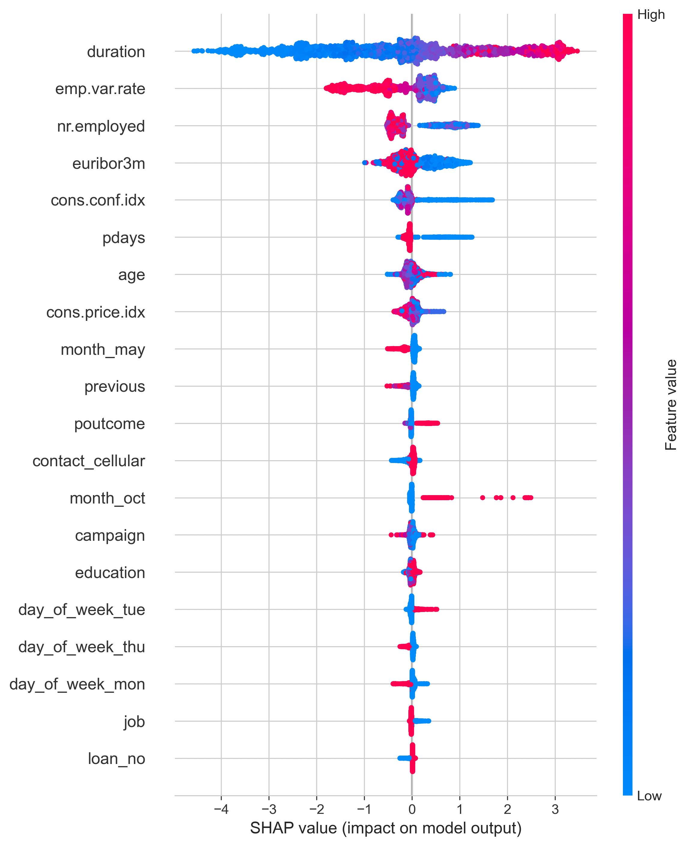
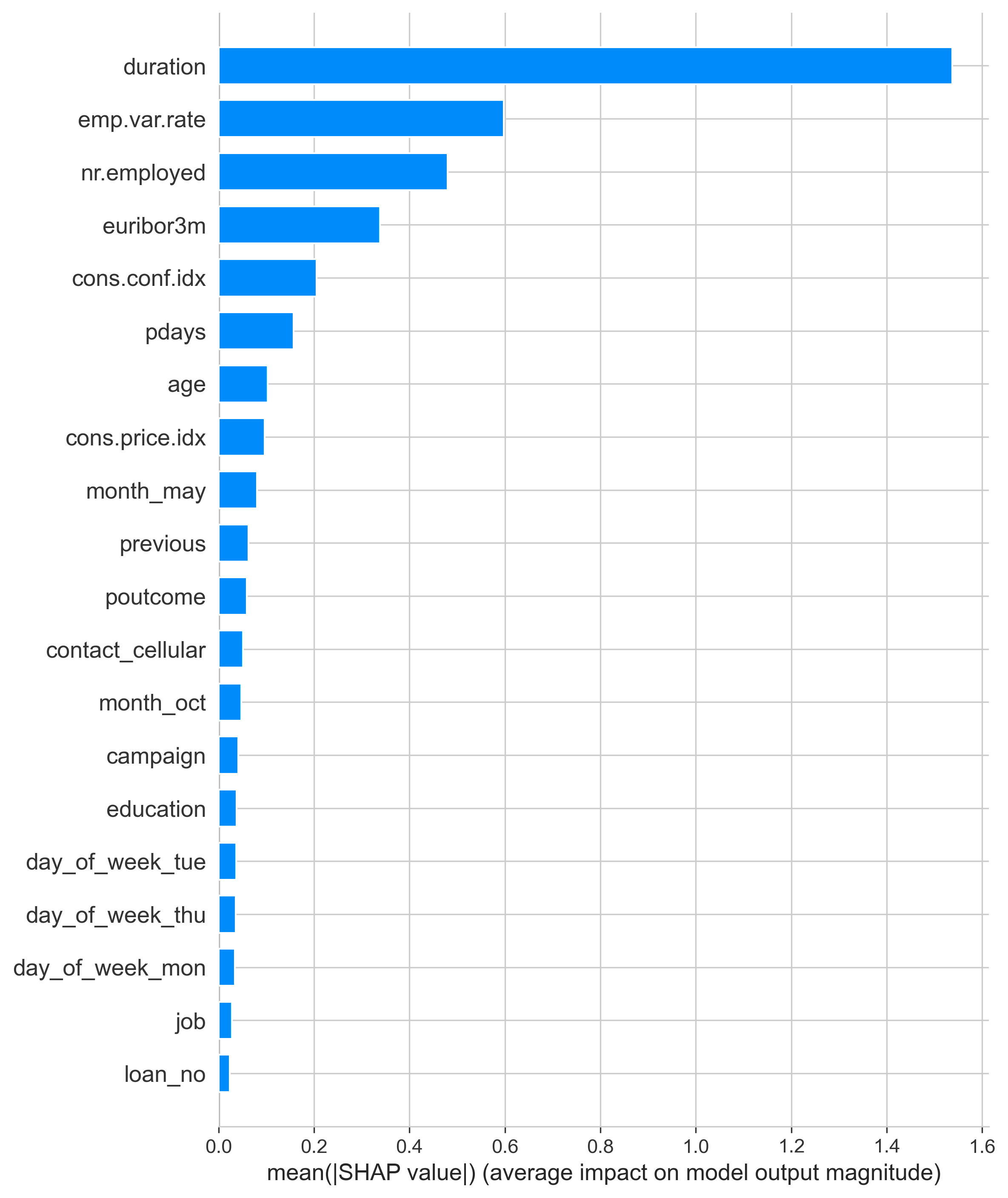
Figure 10 displayed the columns ranked by their mean SHAP values. In this, duration clearly came out on top with emp.var.rate, nr.employed, euribor3m, and cons.conf.idx trailing behind it. Duration had a mean value of around 1.5 making it clearly the most impactful column with the next variable having only a score of 0.6, showing that it still is impactful, but duration is by far the most useful for outcome prediction.

After this process, we took the top contributors and hyperparameter tuned them with the model being XGBoost and the method of handling the imbalanced dataset being undersampling since these two combined yielded the best results. The only columns that were used in this test were duration, emp.var.rate, nr.employed, euribor3m, cons.conf.idx, pdays, and age. The ending parameters were 0.4, 0.05, and 0.5 being col_samplebynode, eta, and subsample respectively. The results, as shown in table 5 were very similar to the results of table 3, with barely any score differences in the testing portion. This shows that the seven columns listed above were the main factors in predicting the outcomes of the dataset.

Table 6. Summary of evaluation metrics of the tuned XGboost model using undersampled data and only using the seven columns with the highest SHAP scores

Model	Handling Imbalance	Train/Test	Outcome	Precision	Recall	F1	AUC
XGBoost (colsample_bynode: 0.4 eta: 0.05 subsample: 0.5)	Undersampled	train	0	92.4 ± 0.2	83.2 ± 0.3	87.6 ± 0.2	93.8 ± 0.1
			1	84.7 ± 0.2	93.2 ± 0.2	88.8 ± 0.1	93.8 ± 0.1
		test	0	92.4 ± 1.5	81.7 ± 2.1	86.7 ± 1.4	93.2 ± 1.0
			1	83.6 ± 1.9	93.2 ± 1.3	88.2 ± 1.3	93.2 ± 1.0

When comparing this to how the XGBoost undersampled with all the features resulted, we can see that the results were very similar with the scores being 0.91,0.82, 0.86 for precision, recall, and f1 scores respectively for the 0 outcome, and 0.83, 0.92, and 0.87 for the 1 outcome. There was only a difference of 0.01 in scores that were different, meaning that the seven features were in fact, what the models relied on to predict outcomes the most, as with adding the other 20+ features to the model, it only resulted in a 0.01 score increase.

We have realized however, that duration won’t be known before the call, leading the model to not have one of its key data points in prediction. This realization made us remove the duration variable from the dataset while using the XGBoost model and undersampled data in order to get a more life-accurate prediction.

Table 7. Using top seven columns (not including duration) with highest SHAP scores of the tuned XGBoost model using undersampled data.

Model	Handling Imbalance	Train/Test	Outcome	Precision	Recall	F1	AUC
XGBoost (colsample_bynode: 0.35 eta: 0.05 subsample: 0.4)	Undersampled	train	0	71.9 ± 0.2	83.6 ± 0.3	77.3 ± 0.2	80.4 ± 0.2
			1	80.5 ± 0.3	67.5 ± 0.4	73.3 ± 0.3	80.4 ± 0.2
		test	0	72.2 ± 2.2	85.5 ± 1.9	78.3 ± 1.7	81.1 ± 1.7
			1	82.3 ± 2.3	67.1 ± 2.6	73.9 ± 2.1	81.1 ± 1.7

From this data, we can see that the scores had a decent drop with the outcomes of 0 being 72.2 ± 2.2, 85.5 ± 1.9, and 78.3 ± 1.7 for precision, recall, f1, and AUC scores respectively, with the outcomes of 1 being 82.3 ± 2.3, 67.1 ± 2.6, 73.9 ± 2.1, and 81.1 ± 1.7 for the same respective scores. The precision scores for an outcome of 0 dropped noticeably from this test to the test that included the duration score, with the recall score of the same outcome going up by 0.2. However, this is the opposite for outcomes of 1 where precision only went down slightly, while recall lowered at a much greater value. From this, we can see that without knowing the duration in a more lifelike situation, the model is more inaccurate in its predictions than it was before with duration, but still is somewhat accurate.

Earlier in the exploratory data analysis, we mentioned that emp.var.rate and euribor3m had extremely high correlation scores, making us wonder whether we are able to remove one of these variables from our model. We decided to try removing euribor3m to determine whether the model would be heavily impacted from losing a highly important variable because of how correlated the two features are.

Table 8. Using a dataset without euribor3m with the tuned XGBoost model using undersampled technique.

Model	Handling Imbalance	Train/Test	Outcome	Precision	Recall	F1	AUC
XGBoost (colsample_bynode: 0.35 eta: 0.05 subsample: 0.4)	Undersampled	train	0	92.0 ± 0.2	82.9 ± 0.3	87.2± 0.2	93.6± 0.1
			1	84.5 ± 0.2	92.7 ± 0.2	88.4 ± 0.1	93.6 ± 0.1
		test	0	91.5 ± 1.6	81.6 ± 2.1	86.3 ± 1.5	93.1 ± 1.0
			1	83.4 ± 2.0	92.4 ± 1.4	87.7 ± 1.3	93.1 ± 1.0

When comparing these results to what was gotten from the original undersampled model, we can see that the results of every f1-score went down by around 0.4. It went from 86.7 ± 1.4 to 86.3 ± 1.5 and 88.2 ± 1.2 to 87.7 ± 1.3 for test outcomes of 0 and 1 respectively. The AUC scores only decreased by 0.1 (from 93.2 ± 1.0 to 93.1 ± 1.0). This result proves our theory that without euribor3m, the model would act mostly the same due to how high the correlation scores were between the feature and emp.var.rate.

Conclusion

The objectives of this study were to determine the most effective machine learning model, along with the best method of balancing the dataset. Furthermore, we strived to understand and quantify the effect of the features related with bank telemarketing on model predictions. With this information, banks would be able to better understand which factors are most impactful in telemarketing success, along with being able to target certain demographics based on the outcomes of our study. The features with the highest contributions and impacts will be focused on the most, while other, less impactful features will be considered less when reaching out to customers for a telemarketing campaign.

In order to achieve our goal of finding the best method of balancing the dataset, we use three different methods: balancing the class weights in the algorithm, undersampling, oversampling (SMOTE), and a mix of the last two techniques. Balancing the dataset was needed to have the best outcomes due to the high discrepancy between the successes and failures in the dataset. The successes had around 4,101 while the failures had 27,727 values in the dataset. Without balancing the dataset, the model would heavily favor the failures due to it having a significantly larger presence in the dataset.

The models themselves also needed tweaking in order to achieve the strongest results. A method called hyperparameter tuning was used in which values are given to parameters allowing the model to focus on different parts, changing the outcomes of algorithms. This was used on both random forest and XGBoost, giving us the most accurate results. Additionally, neural networks utilized a custom cross-entropy loss function used to hopefully give better results. In the end, the undersampled XGBoost model was considered the best model out of the batch due to the high f1 score average of 0.87 and 0.88 for outcomes of 0 and 1, respectively. While random forest with undersampling yielded similar results, we held XGBoost at a higher regard due to it having less overfitting than the random forest model. The neural network models didn’t achieve better results than the one XGBoost resulted in.

The findings in the study can’t compare with the first two studies aforementioned at the beginning of this as the paper written by Moro et al. used a completely different metric of decisions, along with mostly completely different models besides neural networks. This same sentiment is kept with the paper written by Ilham et al. as their study consisted of the same decision metric, along with only two similar models being neural networks and random forest, neither of which ended up being the best model. With both of these models losing, a thin line of similarities can be drawn between our findings and their findings, random forest and neural networks were both not the most effective model in our findings. For Bogireddy et al.’s⁵ findings however, we use very similar evaluation metrics of f1-score, however they also use an accuracy score, which as already mentioned, isn’t as accurate as the f1-score evaluation metric. Their results also found that XGBoost yielded the greatest results in model prediction accuracy, which is the same as our findings. They only used SMOTE as a data imbalancing technique though, which can explain why the results our XGBoost model found were better than those found by their model. Peter et al.’s⁶ model again used different evaluation metrics which also shows that their results aren’t fully accurate and can’t be put up against our results.

SHAP values, which quantify the impact each variable has on the model output along with correlation values, gave us a better understanding of the features importance on the predictions. Ranking the features from greatest to least in accordance to their SHAP values allows us to determine which variable was the most impactful in determining whether a telemarketing campaign would succeed or fail on a customer. The results were duration having the greatest SHAP value, followed by emp.var.rate, nr.employed, eribor3m, and cons.conf.idx. The rest of the values were relatively negligible due to the values being very low. This means that some of these variables could potentially be removed without affecting the model greatly due to them being relatively similar. Because of how much higher the five given features’ SHAP values were compared to the rest of the variables, the data shows that these five values were the most impactful in model prediction. We can then draw a conclusion that whichever model could most effectively consider and use these five metrics in their predictions, would result in the highest scores. This means that XGBoost was the best at using these features in model prediction.

Some limitations for this study, however, are both the number of models we used and the parameters of each model that were hyperparameter tuned, along with the configuration of the neural network model. In this study we only use 3 different machine learning models being XGBoost, random forest, and neural networks. This low number in itself is a limitation as there is a high likelihood of other models being available which do yield better results. Additionally, within each model, the configuration of each model was the best we found, however there could still be more effective configurations which could be found if given unlimited time. Future studies can address these limitations by either adding more models, or simply trying to better optimize the models used in this study.

References

1. Sabadi, I. (2025, May 7). What is the conversion rate in telemarketing? Actual data 2025. Verificaremails. https://www.verificaremails.com/en/what-is-the-conversion-rate-in-telemarketing-actual-data-2025/ [↩]
2. An, F. (2024, December 24). 10 best practices for sales and telemarketing success. Sobot.io. https://www.sobot.io/article/sales-telemarketing-best-practices/ [↩]
3. Research and Markets. (2025). Outbound telemarketing – Global strategic business report. https://www.researchandmarkets.com/report/outbound-telemarketing [↩]
4. Ilham, A., Khikmah, L., Indra, U., & Iswara, I. B. A. I. (2019, March). Long-term deposits prediction: A comparative framework of classification model for predict the success of bank telemarketing. Journal of Physics: Conference Series, 1175, 012035. https://doi.org/10.1088/1742-6596/1175/1/012035 [↩] [↩]
5. Bogireddy, S. R., & Murari, H. (2024). Machine learning for predictive telemarketing: Boosting campaign effectiveness in banking. 2024 International Conference on Power, Energy, Control and Transmission Systems (ICPECTS), 1–6. https://doi.org/10.1109/ICPECTS62210.2024.10780120 [↩] [↩]
6. Peter, M., et al. (2025). Predicting customer subscription in bank telemarketing campaigns using ensemble learning models. Machine Learning with Applications, 19, 100618. https://doi.org/10.1016/j.mlwa.2025.100618 [↩] [↩]
7. Moro, S., Cortez, P., & Rita, P. (2012, February 13). Bank marketing. UCI Machine Learning Repository. https://archive.ics.uci.edu/dataset/222/bank+marketing [↩]
8. Chawla, N., Bowyer, K., Hall, L., & Kegelmeyer, W. (2002). SMOTE: Synthetic minority over-sampling technique. arXiv, abs/1106.1813. https://www.semanticscholar.org/paper/SMOTE%3A-Synthetic-Minority-Over-sampling-Technique-Chawla-Bowyer/8cb44f06586f609a29d9b496cc752ec01475dffe [↩]
9. Gu, P., & Lu, Y. (2024). A hybrid active sampling algorithm for imbalanced learning. 2024 27th International Conference on Computer Supported Cooperative Work in Design (CSCWD), 600–605. https://doi.org/10.1109/CSCWD61410.2024.10580268 [↩]
10. Breiman, L. (2001). Random forests. Machine Learning, 45, 5–32. https://doi.org/10.1023/A:1010933404324 [↩]
11. Chen, T., & Guestrin, C. (2016). XGBoost: A scalable tree boosting system. Proceedings of the 22nd ACM SIGKDD International Conference on Knowledge Discovery and Data Mining, 785–794. https://doi.org/10.1145/2939672.2939785 [↩]
12. Kriegeskorte, N., & Golan, T. (2019, April). Neural network models and deep learning. Current Biology, 29(7), R231–R236. https://doi.org/10.1016/j.cub.2019.02.034 [↩]
13. Deepchecks. (2022, December 22). What is precision in machine learning. https://www.deepchecks.com/glossary/precision-in-machine-learning/ [↩]
14. Iguazio. (2024, February 15). What is recall. https://www.iguazio.com/glossary/recall/ [↩]
15. Frank, E. (2023, April 29). Understanding the F1 score. Medium. https://ellielfrank.medium.com/understanding-the-f1-score-55371416fbe1 [↩]
16. Dash, S. (2022, October 19). Understanding the ROC and AUC intuitively. Medium. https://medium.com/@shaileydash/understanding-the-roc-and-auc-intuitively-31ca96445c02 [↩]
17. Rathi, D. (2024, October 14). Handling imbalanced data: Key techniques for better machine learning. Medium. https://medium.com/@dakshrathi/handling-imbalanced-data-key-techniques-for-better-machine-learning-6e33b466f8b7 [↩]
18. Belcic, I., & Stryker, C. (2024, July 23). Hyperparameter tuning. IBM. https://www.ibm.com/think/topics/hyperparameter-tuning [↩]
19. Lundberg, S., & Lee, S. (2017). A unified approach to interpreting model predictions. Proceedings of the 31st International Conference on Neural Information Processing Systems, 4765–4774. https://dl.acm.org/doi/10.5555/3295222.3295230 [↩]