Leveraging Machine Learning for Predicting NBA Player Performance

Abstract

Artificial Intelligence (AI) and Machine Learning (ML) can be used in sports analytics for predicting numerous statistics, especially player performance. One specific application would be predicting a certain NBA player’s points scored in a certain game. AI can help with capturing complex, non-linear patterns that player points per game can follow. Our study used four machine learning models, linear regression, neural networks, decision tree regressors, and random forest regressors, to predict NBA player points. A combined model was developed to combine the best of all individual models. The results have low errors and a high degree of accuracy in points predicted. This is an indicator that AI is indeed an effective method in determining player statistics for an upcoming game that can have a positive impact on planning and strategizing for future games.

Introduction

Background and Context

Artificial Intelligence (AI) has significantly transformed various industries, including sports analytics, where it plays a crucial role in predicting game outcomes and player performances. In the realm of NBA basketball, the application of AI and Machine Learning (ML) models has the potential to revolutionize how teams strategize and evaluate player performance. By leveraging large datasets and sophisticated algorithms, AI can uncover patterns and trends that are not immediately apparent through traditional analysis methods.

The systematic review in¹ identified a number of AI and ML techniques used for predicting the outcomes of basketball games. Hybrid Fuzzy-SVM model² determines which team is going to win a certain game. Other papers apply AI to the general field of sports analytics are in^3,4,5,6. ​Artificial intelligence (AI) is transforming sports analytics by enhancing performance analysis, injury prediction, and game strategy optimization³.⁴ It has been highlighted that AI is revolutionizing sports analytics by improving key areas such as performance evaluation, injury forecasting, and strategic planning. A systematic review of 72 studies on machine learning applications in sports found a significant shift from classical techniques to deep learning methods in recent years⁵. Another study⁶ ​shows that artificial intelligence (AI) has significantly transformed sports analytics by enhancing decision-making and forecasting capabilities.

On the subject of sports analytics, basketball metrics used in National Basketball Association (NBA) and EuroLeague games have been reviewed⁷. The paper found that although a lot of data existed, tools that could forecast players’ performance were lacking. Some useful metrics including Player Impact Estimate (PIE), Net Rating (NetReg), and Player Efficiency Rating (PER) were discussed. A forecasting scenario that utilized data from three basketball seasons was discussed. Based on the player statistics available, the paper predicted the MVP and the Top Defender by computing an Aggregated Performance Indicator (API) and a Defensive Performance Indicator (DPI) respectively. The specific metric of PER has been studied further in⁸. Using three AI models, Lasso Regression, Random Forest Regression, and Neural Networks, they adjust the weights for each statistical component used in computing PER. Their goal is to compute PER more accurately.

Problem Statement and Rationale

In Section 1.1, we discussed the overall context of our work: sports analytics in basketball. Existing tools either refine statistical metrics or predict who will win awards such as MVP. However, to the best of our knowledge, there is no prior work that attempts to predict the number of points scored by an individual player. Our paper attempts to answer the following questions: Given a set of attributes from past games for the players involved, can we predict the number of points scored by a given player in an upcoming game? How do some machine learning techniques perform when used for this prediction?

Significance and Purpose

Forecasting in sports⁷ is widely used for improving the performance of teams in upcoming games. While computed measures such as Player Efficiency Rating (PER) are useful for understanding the impact a player may have, specific attributes such as points scored or rebounds collected provide a much more direct picture of a player’s expected impact. As discussed in⁸, there are disagreements regarding how best to compute these derived attributes as they are being constantly refined. Unlike prior work, our paper explores whether AI models can accurately predict a specific attribute after the models have been trained with historical data. If these predictions are accurate enough, then coaches can use the forecasts for an upcoming game against a certain opponent. For example, they can decide on a starting lineup with players with the maximum values of the critical attributes against a particular opposing team.

Contributions

This paper uses machine learning models to predict a basketball player’s score in an upcoming game, a novel contribution to the best of our knowledge. A combined model is developed to obtain the best of all individual models. Experimental results are presented that use error values and points predicted to compare the models’ accuracy. Results overall show that these techniques can be highly effective as a predictor of points scored, impacting planning and strategizing for upcoming games.

The rest of the paper is structured as follows: Section 2 introduces the individual and combined models, and the dataset used in our study. Section 3 discusses the model configurations, the evaluation methodology, and results including the predicted points per game. Section 4 concludes with key findings, potential impact, and possible future work.

Methodology

Research Design

Our paper contains research and an experimental component. We build 4 machine learning models to analyze data from prior basketball matches and predict how many points a player would score in an upcoming match. We build an ensemble technique to combine results from the individual models and predict a player’s score — the goal is to utilize the best of all the models. We use datasets available for games played in the National Basketball Association (NBA) for evaluating the models and the ensemble method. 

Approach for Choosing AI Models

This study utilizes multiple machine learning models, each offering unique strengths in analyzing and predicting player performance. Linear regression, neural networks, decision tree regressors, and random forest regressors are employed to capture different aspects of the data. 

Each of these models has its own strengths which makes it suitable for this research. Linear regression models are simple and easy to interpret, and are a good baseline to compare other models to. Additionally, it is much faster and less prone to overfitting, and gives clear coefficients to help understand how separate features affect the result. 

The neural network captures complex nonlinear relationships which wouldn’t be caught by linear models, and works better than other regressors (ridge, lasso) to find intricate patterns.

 Decision trees also capture non-linear relationships between features, and can easily be visualized and interpreted. Unlike k-NN or SVMs, decision trees don’t require feature scaling or distance metrics. Additionally, there is less computational cost than ensemble methods such as gradient boosting. 

Random forests are an ensemble of decision trees, and reduces overfitting which can be commonly seen among single trees. Additionally, it frequently outperforms other models such as Naive Bayes on structured data such as the ones used in this research.

The use of an ensemble approach, combining predictions from these models, aims to enhance overall predictive accuracy. The multiplicative weight update algorithm is introduced in Section 2.6 (e) to integrate the predictions from various models, penalizing those with larger errors to improve the final prediction. 

Data Collection

The NBA is the premier basketball league in the world. There are 30 teams, and each team has around 15 players. The dataset used in this study consists of comprehensive player statistics from the 2023-2024 NBA season⁹. The above dataset contains data for around 400 players, with one entry per player. The dataset encompasses the following key features where other than the first attribute, all the others are averages over the entire season.

• Games Played: The number of games a player has participated in during the season.
• Minutes Played per game: The average minutes per game a player has spent on the court.
• Field Goals Attempted per game: The average number of field goals a player attempted per game.
• Three-Point Attempts per game: The average number of three-point shots attempted by the player per game.
• Two-Point Attempts per game: The average number of two-point shots attempted by the player per game.
• Free Throws Attempted per game: The average number of free throws attempted by the player per game.
• Total Rebounds per game: The average number of rebounds a player has collected per game.
• Steals per game: The average number of steals made by the player per game.
• Points per game: The target variable, representing the points scored by the player in a game on average.

Based on past data, statisticians do their best to predict the number of points scored in the next game, along with individual player stats. The features in our chosen dataset provide a robust basis for training and evaluating the predictive models. The dataset allows for an in-depth analysis of how different player statistics contribute to scoring performance. By utilizing this data, the study aims to develop accurate models for predicting NBA player points and understand the factors influencing scoring output.

The dataset is split into two categories: the training set and the testing set. The training set takes up 80%, while the testing set takes up the remaining 20%. The training set is used to fit the model. It is going to be used several times to improve training accuracy. The number of times it is used depends on the epochs used to train the model. Certain attributes in our dataset were unlikely to be beneficial to our prediction, so they were not used. Other than that, there were no missing values, normalization, or feature scaling, so no other preprocessing was required. The test set is only going to be seen by the model once, and is used to evaluate final accuracy.

Applicability of the Chosen Dataset for our Study

The intuition behind our work is to predict a player’s score in an upcoming game based on the aggregate data from past games. For a given player P, this aggregate data could be the average of attributes from past games for that player P. For the test dataset used in our study, the non-target attributes are averages over the entire season for a player P. We believe that an average value of a non-target attribute approximates the aggregated data that we need for our work.

Variables and Measurements

The models were evaluated using Mean Squared Error (MSE) as the primary metric. MSE is computed as the average of the error squared. MSE is known for its ability to emphasize larger errors. Lower MSE values indicate higher accuracy. For additional context, model performance was also assessed using training MSE to measure overfitting.

Additionally, we used Mean Absolute Error (MAE) which is simply computed as the average of the absolute errors. MSE and MAE were selected because they provide a clear, direct, and robust assessment of prediction error. MAE offers easy interpretation in the same units as the target variable (points), while MSE ensures that larger errors are penalized more, which is useful for refining model accuracy. R² and RMSE were excluded due to potential misinterpretation, redundancy, or less practical value in the specific context of individual basketball player scoring prediction.

Overfitting refers to fine-tuning of a model to specifically fit a certain data. In order to ensure that our model was not overfitted, we looked at both training and testing MSEs, and if there was a large difference between the two, it can be determined that the model is prone to overfitting.

By training on the entire dataset (aside from the final test games), we ensured the model could fully capture the nuanced scoring trends and contextual variations in the player’s season. While this approach may increase the risk of overfitting, it was a deliberate trade-off to prioritize pattern recognition and prediction accuracy over generalization, since the target was one player’s performance, not team-level or league-wide trends.

Materials and Methods

To predict NBA player points, four machine learning models were developed and evaluated: linear regressor, neural networks, decision tree regressors, and random forest regressors. Each model was chosen for its distinct capabilities in capturing various aspects of the data and predicting player performance. It is unlikely that any unintended bias arose from our models.

a) Linear Regressor

Linear regression is a fundamental statistical method used to model the relationship between a dependent variable and one or more independent variables. The model assumes a linear relationship between the input features and the target variable, which in this study is the points scored by NBA players.

The linear regression model is represented by the equation:

   

where:

• y is the target variable (points scored),
• β₀ is the intercept,
• ​β₁, β₂, …, β_n are the coefficients for each feature,
• x₁, x₂, …, x_n​ are the input features,
• ϵ represents the error term.

The goal of linear regression is to estimate the coefficients that minimize the sum of squared residuals. This model is valued for its simplicity, interpretability, and efficiency. However, it assumes linear relationships, which may not capture more complex patterns in the data.

b) Artificial Neural Network

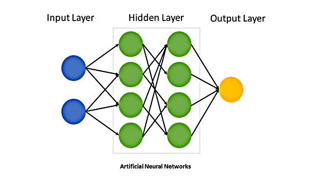
Neural networks are inspired by the human brain’s architecture and are designed to model complex, non-linear relationships between input features and the target variable. A typical neural network consists of an input layer, one or more hidden layers, and an output layer. Each layer contains neurons that perform linear transformations followed by non-linear activation functions. A diagram of an artificial neural network is provided in Figure 1. The network’s output is computed as:

   

   

where:

• x_i are the input features,
• w_ij are the weights between input and hidden layers,
• h_j are the activations of the hidden layer,
• f is the activation function (e.g. ReLU, sigmoid),
• w_j​ are the weights between hidden and output layers,
• b_j and b are the bias terms.

Neural networks are capable of capturing intricate patterns in data and are well-suited for tasks with complex relationships. However, they can be prone to overfitting and require significant computational resources.

c) Decision Tree Regressor

The decision tree regressor models the target variable by recursively splitting the data based on feature values. The tree structure consists of nodes where each internal node represents a decision and each leaf node represents a predicted value.

The decision tree is built as follows:

1. Root Node: The entire dataset is split based on the feature and threshold that minimize variance.
2. Recursive Splitting: The data is split further at each node until a stopping criterion is met.
3. Prediction: For new data, the model traverses the tree to reach a leaf node with the predicted value.

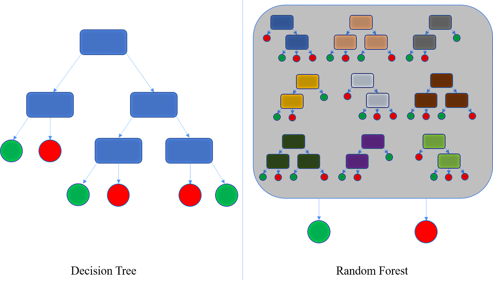
Decision trees are intuitive but cannot capture non-linear relationships. Additionally, they may suffer from overfitting and instability. A diagram of a decision tree is provided on the left side of Figure 2.

d) Random Forest Regressor

The random forest regressor is an ensemble method that combines multiple decision trees to improve accuracy and robustness. It constructs multiple decision trees on different subsets of data and averages their predictions. The process involves:

1. Bootstrapping: Creating multiple bootstrap samples from the original dataset.
2. Tree Construction: Training decision trees on these samples using random subsets of features.
3. Aggregation: Averaging predictions from all trees to obtain the final prediction.

Random forests avoid the limitations of individual trees, such as overfitting, and provide a more stable and accurate model. A diagram of a random forest is provided on the right side of Figure 2.

e) Combining Models with Multiplicative Weight Update Algorithm

To improve prediction accuracy, a multiplicative weight update algorithm was employed. This algorithm adjusts the weight of each model based on its prediction accuracy, combining their outputs to enhance overall performance. The model penalizes worse models while determining the weighted average, which works to improve overall accuracy. Our weight-update algorithm is inspired by the Hedge Algorithm¹⁰, which is a well-known strategy used for combining results from different experts (or models). It assigns weights to each expert based on past performance. The connection between the Hedge Algorithm and our technique is further described below.

The algorithm operates as follows:

1. Initial Weights: Assign equal initial weights to all models.
2. Prediction and Error Calculation: Calculate the error for each model’s prediction.
3. Weight Adjustment: Update the weight of each model using ½ⁿ​, where n is the error magnitude. As mentioned above, our method is based on the Hedge Algorithm¹⁰ that updates weights using an exponential weighting scheme. As the Hedge Algorithm penalizes poorly performing experts by reducing their weights, our algorithm significantly lowers the importance of models with large errors by using the weighting function of 1/2ⁿ. Instead of using e as in the Hedge Algorithm, our technique uses 2 because it is a close approximation of e.
4. Normalization: Normalize weights to sum to one.
5. Ensemble Prediction: Combine model predictions using weighted averages.

This approach leverages the strengths of each model while addressing their weaknesses, resulting in improved prediction accuracy. The multiplicative weight update is a post training algorithm, which means it takes results of models after they’ve already been trained. This is why it was chosen over traditional ensemble methods such as stacking or boosting, since those combine models given a prior formation.

Results and Evaluation

Parameters and Model Configurations

Each machine learning model was tuned to optimize performance, employing hyperparameter tuning to achieve the best results. A random search method was employed, rather than a grid search. This indicates that parameters were initially randomly decided and adjusted based on their performance. 

Although early stopping and validation sets were not used during training, running the neural network for a full 200 epochs allowed us to maximize learning from a relatively small dataset. Many numbers of epochs were experimented with and the results determined that 200 was an ideal number which allowed for training to happen quickly while still maintaining proper accuracy. Given that our dataset was limited to just a few hundred players’ statistics, introducing a validation set would have further reduced the size of the training data, potentially weakening the model’s ability to learn from available patterns. Below are the key parameters used for each model:

1. Linear Regression: No hyperparameters required tuning for basic implementation.
2. Neural Network

• Architecture: 1 input layer, 2 hidden layers, and 1 output layer.
• Activation Function: ReLU for hidden layers, linear activation for output.
• Epochs: 200 (to balance training time and accuracy).
• Batch Size: 32.

3. Decision Tree Regressor

• Maximum Depth: 42.
• Minimum Samples per Leaf: 1.

4. Random Forest Regressor

• Number of Trees: 100.
• Maximum Depth: 42.
• Minimum Samples per Split: 2.

Future work may incorporate early stopping and validation strategies once a larger or multi-player dataset is available. However, in this context, the decision to train for 200 full epochs was a practical and beneficial choice that yielded strong performance on the test set.

Dataset and Implementation Overview

To evaluate the performance of the machine learning models, we utilized a dataset consisting of player statistics from the 2023-2024 NBA season⁹, as mentioned in Section 2. The dataset was split into a training set (80%) and a testing set (20%). The training set was used to fit the machine learning models, while the testing set provided an independent evaluation of model performance.

Our project utilized pandas¹¹ for data manipulation, NumPy¹² for numerical computations, and Scikit-learn¹³ for the individual machine learning models. Additionally, TensorFlow¹⁴ with Keras¹⁵ was employed to create and train a neural network. The MSE and MAE for the multiplicative weight update algorithm are computed from that of the individual models.

All models were implemented in Python 3.11 using the Visual Studio Code (VSCode) environment. The primary libraries used included pandas 2.2.2 for data manipulation, NumPy 1.26.4 for numerical operations, and scikit-learn (sklearn) 1.6.0 for model training, evaluation, and preprocessing. The neural network model was implemented using scikit-learn’s MLPRegressor, which is suitable for shallow feedforward networks.

The code for our implementation is available freely on GitHub¹⁶. All the experiments were run using an AMD Ryzen 7 7730U with Radeon Graphics running at 2.00 GHz, containing 32.0 GB of memory, running on Windows 11 Pro Version 23H2. No GPUs were used for running the experiments.

Model	Training MSE	Testing MSE	Training MAE	Testing MAE	Observations
Linear Regression	2.21	2.50	1.12	1.29	Simple model; struggles with capturing non-linear relationships.
Neural Network	1.72	1.85	0.94	1.07	Effective at identifying complex patterns; minor overfitting observed.
Decision Tree Regressor	1.11	1.72	0.59	1.02	Strong performance; prone to overfitting when trained without restrictions.
Random Forest Regressor	1.60	1.67	0.80	0.96	Best overall performance due to ensemble approach and reduced overfitting compared to decision trees.
Combined Model	–	1.70	–	1.00	Effective aggregation; slightly less accurate than the best single model (Random Forest).

Model Comparison using MSE, MAE, and Actual vs Predicted PPG

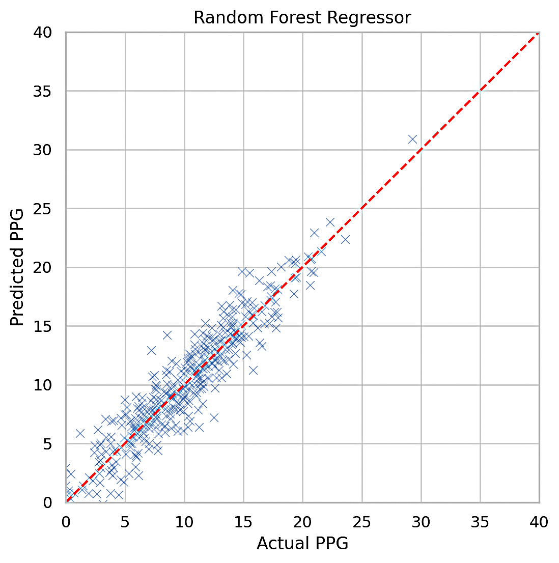
We discussed MSE and MAE in Section 2.5, Variables and Measurements. Table 1 shows the training and testing MSE and MAE values for all the models. The idea is to compare the overall error metrics, the lower being better. Figures 3, 4, and 5 plot the actual vs predicted Points Per Game (PPG). Perfect prediction is shown as a straight line, so clustering around that line indicates better accuracy.

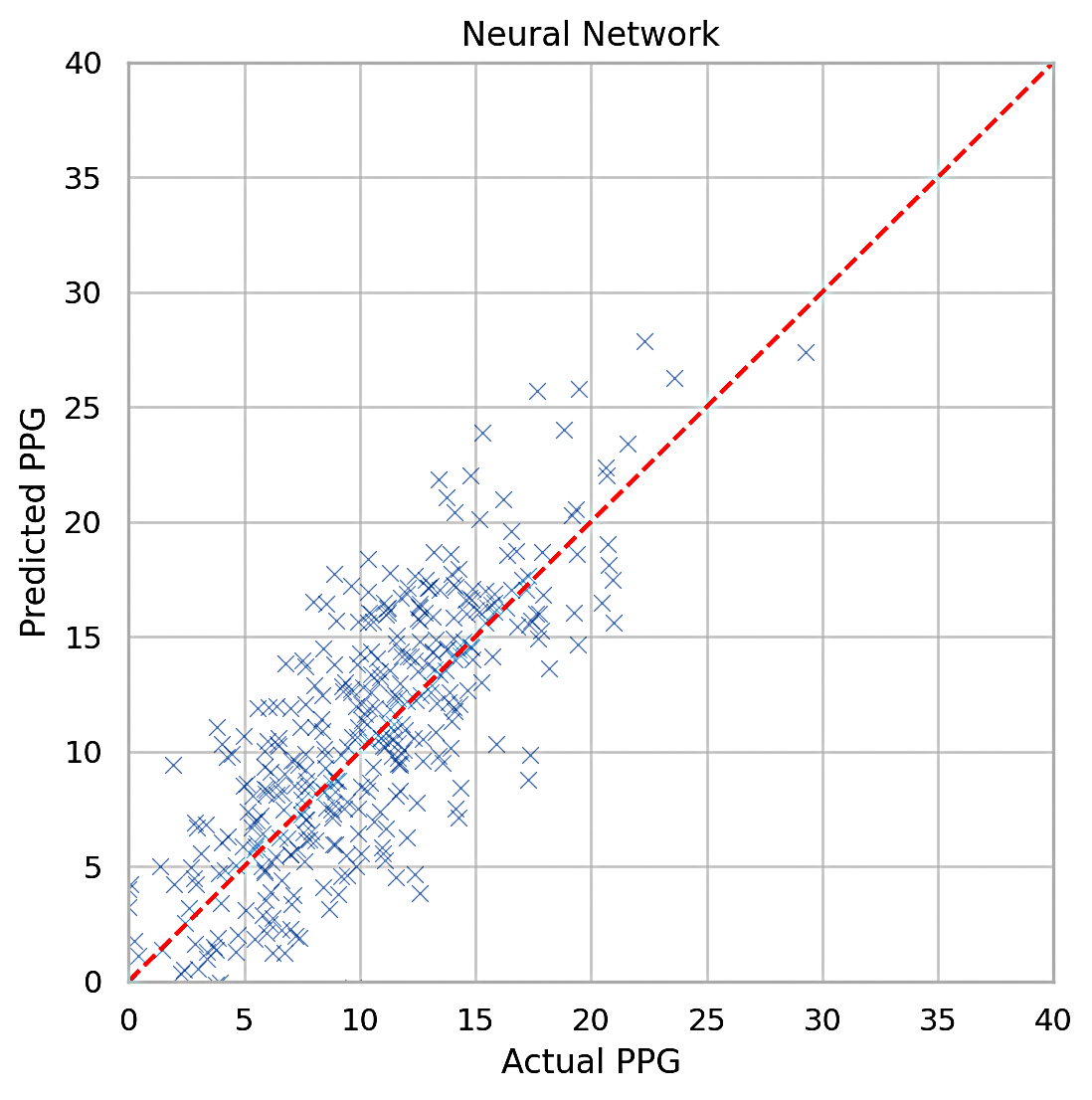
Linear Regression: The results display that linear regression is effective, but it is not a great way to get the best results every single time. It leads to deviations from the true result, and it isn’t extremely effective. Linear regression yielded the highest testing MSE (2.50), reflecting its limitations in capturing the non-linear relationships between input features and points scored. However, its simplicity and speed make it a useful baseline for comparison. Actual vs predicted PPG results (shown in Figure 3) confirm that linear regression may be less suited for modeling complex sports data.

Neural Network: Based on our results, the neural network is a good method for predicting points, but it is not the most effective method. This may be due to randomness in the data set, which makes it difficult to capture a proper pattern within the dataset. The neural network outperformed linear regression with a testing MSE of 1.85, a fact confirmed by the PPG visualizer in Figure 3. The network’s architecture, featuring two hidden layers, enabled it to capture complex patterns in the data. However, the slight gap between training MSE (1.72) and testing MSE indicates minor overfitting, which could be addressed through regularization or dropout techniques.

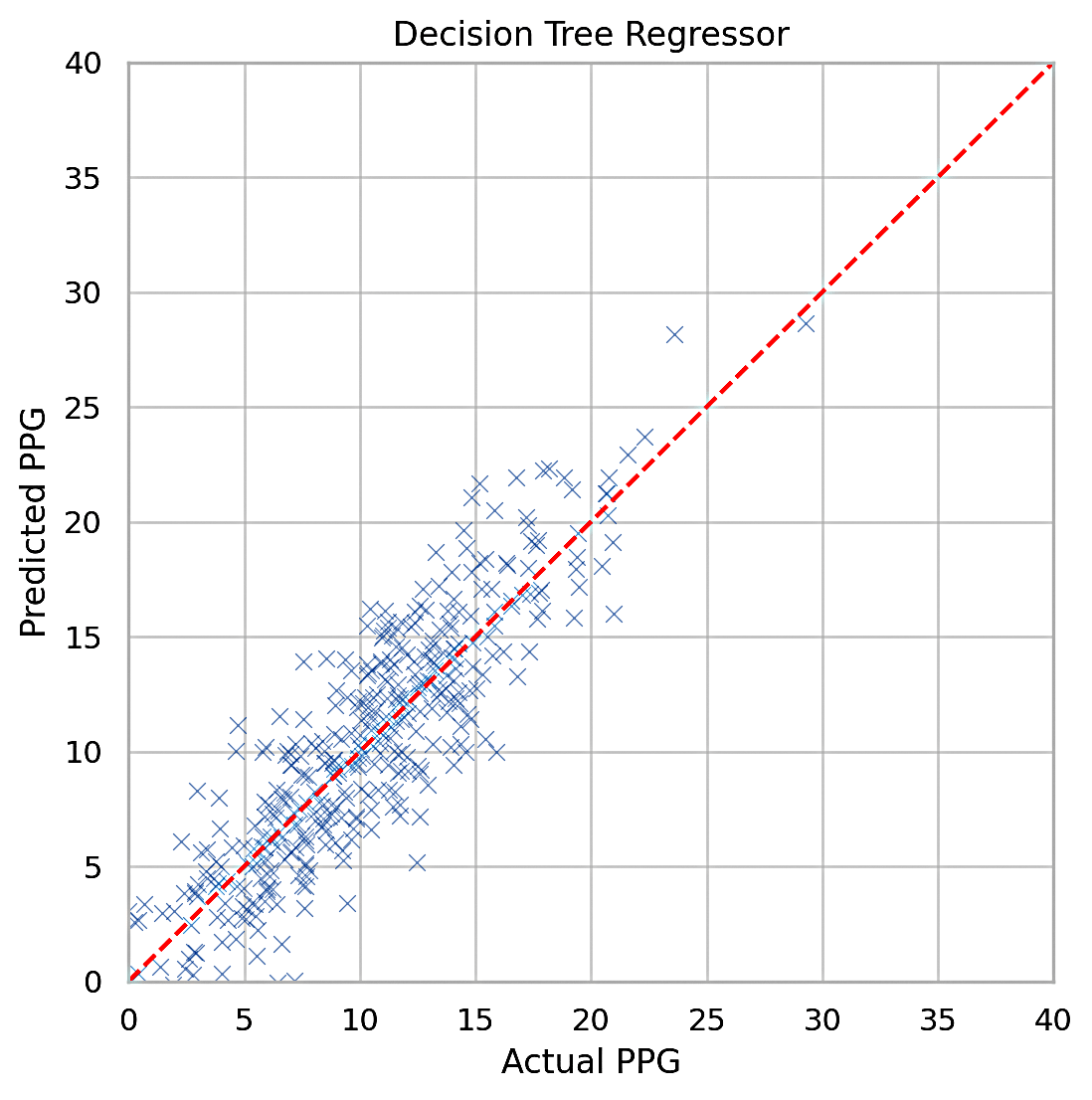
Decision Tree Regressor: The decision tree regressor demonstrated strong predictive power, achieving a testing MSE of 1.72. The tree’s ability to split data based on feature importance contributed to its success. However, decision trees are prone to overfitting, as shown by the significantly lower training MSE (1.11) compared to the testing MSE.

Random Forest Regressor: According to the results, this is the best model for predicting how many points the player scored. The random forest regressor achieved the best performance, with a testing MSE of 1.67. By averaging predictions from multiple decision trees, the model mitigated overfitting and improved stability. The slight difference between training MSE (1.60) and testing MSE indicates a well-generalized model as is confirmed by the PPG visualizer in Figure 4.

Combined Model (Multiplicative Weight Update Algorithm): According to the results, this model was good but not the best, since it may not be better than the best individual model. For example, if the true number of points was lower than each of the individual predictions, the combined prediction would be worse than at least one of the individual models. 

The combined model, utilizing the multiplicative weight update algorithm, achieved a testing MSE of 1.70. While it effectively aggregated predictions from all models, its performance was slightly inferior to the best single model (random forest). This result highlights the trade-offs inherent in ensemble methods: while they balance errors across models, they may not outperform the top-performing model in isolation. Figure 5 shows that the predicted points-per-game for this algorithm closely hug the perfect prediction line, confirming the effectiveness of this combined model.

Comparative Insights

The results indicate that ensemble methods and non-linear models (e.g., random forest and neural networks) outperform simpler models like linear regression. The random forest regressor emerged as the most accurate model, leveraging its ensemble design to capture complex relationships while avoiding overfitting. The combined model offers a robust alternative for scenarios where individual model predictions are less reliable. The best model which was implemented was the random forest regressor, which had a MAE of 1.3.

The PPG results shown in Figures 3, 4, and 5 indicate high accuracy considering NBA players often vary by 5+ points from game to game. The results show that the predictions track game-to-game fluctuations closely, with most predictions within 3 points of the actual value.

Feature Importance Analysis

To better understand which variables most significantly impact NBA player point predictions, feature importance scores were extracted from the Decision Tree and Random Forest Regressor models. These scores quantify the contribution of each feature to the model’s predictions. Player field goal attempts and minutes played came out as the most influential predictors of a player’s PPG. The Random Forest model, in particular, emphasized field goal attempts as the dominant factor, followed closely by minutes played, suggesting that playing time and scoring opportunities are the primary drivers of scoring.

Model Efficiency and Runtimes

Table 2 lists the training and inference runtimes in seconds for each of the models. The corresponding observations indicate that our models span a spectrum of efficiency, both during training and inference.

Model	Training Time (s)	Inference Time (s)	Runtime Observations
Linear Regression	0.12	0.01	Extremely fast due to closed-form solution; ideal for quick deployment.
Neural Network	42.5	0.47	Slower training due to backpropagation; inference remains acceptable.
Decision Tree Regressor	1.73	0.05	Fast training and inference; runtime increases with tree depth.
Random Forest Regressor	6.88	0.22	Moderately longer due to ensemble of trees; parallelizable.
Combined Model	51.23	0.75	Represents the total training and inference time of all models combined; incurs highest runtime but leverages model diversity for improved accuracy.

Conclusion

Key Findings

This paper explores the application of AI for predicting NBA player statistics, focusing specifically on predicting the number of points scored by a player at a given game. This study highlights the effectiveness of various machine learning models for predicting NBA player points. By implementing linear regression, neural networks, decision tree regressors, and random forest regressors, we assessed their individual strengths and limitations. The combination of these models using the multiplicative weight update algorithm improved overall prediction accuracy. This work underscores the potential of AI in sports analytics and provides a foundation for further research and refinement.

Implications and Significance

This approach provides a comprehensive evaluation of how different models can be combined to achieve more accurate predictions, offering valuable insights for sports analysts and teams. By exploring these models and their combination, the study highlights the potential of AI to improve decision-making and performance analysis in the NBA.

This paper contains several contributions to the field of AI in sports analytics. Namely, we present a technique to accurately predict a player’s points scored in an upcoming game based on their other statistics for past games. Our results using MSE, MAE, and PPG indicate reasonably accurate predictions that should be useful in real life. We also have a method to combine the predictions from multiple artificial intelligence models to leverage the results into a more accurate prediction. Our low error results indicate our success and prove AI’s effectiveness and the predictability of certain player statistics based on other areas of a player’s performance.

Future Directions

Future research could explore more sophisticated ensemble methods, integrate additional features like player injuries and opponent defence statistics, and investigate the effect of real-time data updates. Additionally, examining how external factors impact model performance and experimenting with advanced models like deep learning could further enhance predictive capabilities. Future research could investigate how temporal dependencies or player’s historical performance data were managed or ignored in this prediction model.

Acknowledgments

I would like to thank my mentor, Odysseas Drosis, Cornell University, for his help and guidance during preparation of this paper.

References

1. S. Clementswami et al. Application of artificial intelligence and machine learning to predict basketball match outcomes: A systematic review. Computer Integrated Manufacturing Systems. 28 (11), 998 – 1009, (2022). [↩]
2. S. Jain and H. Kaur. Machine learning approaches to predict basketball game outcome. 3rd International Conference on Advances in Computing, Communication & Automation (ICACCA), pp. 1-7 (2017). [↩]
3. N. Sanghvi, N. Sanghvi et al. Artificial intelligence in sports analytics. International Journal of Engineering Research & Technology (IJERT). 13, Issue 06 (2024). [↩] [↩]
4. I. Ghosh, S. R. Ramamurthy et al. Sports analytics review: Artificial intelligence applications, emerging technologies, and algorithmic perspective. WIREs Data Mining and Knowledge Discovery. 13, Issue 5 (2023). [↩] [↩]
5. V. Vec, S. Tomažič, A. Kos et al. Trends in real-time artificial intelligence methods in sports: a systematic review. Journal of Big Data 11, 148 (2024). [↩] [↩]
6. N. Chmait, H. Westerbeek. Artificial Intelligence and Machine Learning in sport research: an introduction for non-data scientists. Front Sports Act Living (2021). [↩] [↩]
7. V. Sarlis, C. Tjortjis. Sports analytics — Evaluation of basketball players and team performance. Information Systems. 93, Article 101562 (2020). [↩] [↩]
8. R. Seshadri. Improving player efficiency rating in basketball through machine learning. Research Archive of Rising Scholars (preprint) (2024). [↩] [↩]
9. V. Vinco. 2023-2024 NBA Player Stats. https://www.kaggle.com/datasets/vivovinco/2023-2024-nba-player-stats/data (2024). [↩] [↩]
10. W. Krichene, M. Balandat et al. The Hedge algorithm on a continuum. Proceedings of the 32nd International Conference on Machine Learning, Journal of Machine Learning Research: Workshop and Conference Proceedings. 37 (2015). [↩] [↩]
11. The pandas development team. pandas-dev/pandas: Pandas. Version v2.2.2. https://zenodo.org/records/10957263 (2024). [↩]
12. C.R. Harris, K.J. Millman. S.J. van der Walt et al. Array programming with NumPy. Nature 585, 357–362 (2020). [↩]
13. F. Pedregosa et al. Scikit-learn: machine learning in Python. Journal of Machine Learning Research 12 (85):2825−2830 (2011). [↩]
14. M. Abadi et al. TensorFlow: Large-Scale Machine Learning on heterogeneous distributed systems. https://www.tensorflow.org (2015). [↩]
15. Keras: Deep Learning for Humans. https://keras.io/ (2025). [↩]
16. A. Chakrabarti. Machine learning models for predicting NBA player performance. https://github.com/anuragc2030/Machine-Learning-Models-for-Predicting-NBA-Player-Performance (2025). [↩]