Identifying Ocular Diseases Through Classification and Clustering Algorithms

Abstract

Vision is often said to be the most important sense of the human body. However, a large portion of our population have visual impairments and many have still yet to be treated. One method to detect ocular diseases is through the analysis of the patient’s fundus image. However, the task of examining and labelling fundus images is a time-consuming process and requires the need for specialized ophthalmologists who are often scarce in underserved communities¹. In order to address this problem, I have trained and systematically compared machine learning models that are capable of classifying ocular diseases present within a fundus image. By training three Convolutional Neural Network models: ResNet50, DenseNet121 and VGG16 on two datasets belonging to eight and four classes respectively, I have achieved a maximum micro/macro prediction accuracy of 55.73%/45.74% (almost 45%/36% better than random guessing) for dataset one and 90.77%/90.57% (almost 66% better than random guessing) for dataset two. The results of VGG16 and ResNet50, which were comparable, outshined those of DenseNet121. Moreover, I tested the effectiveness of the unsupervised learning model K-means clustering in clustering the two datasets and received an ARI/NMI score of 0.0366/0.1145 for the first dataset and 0.3237/0.4118 for the second. Ultimately, this study can contribute to aiding Ophthalmologists in identifying the early stages of ocular diseases.

Keywords: ResNet50, DenseNet121, VGG16, K-Means Clustering, Ophthalmology, Fundus

Introduction

The human eye is one of the most complex organ systems in our body and is a marvel of evolution and biology. Unfortunately, estimates from the World Health Organization show that a quarter of the world’s population (2.2 billion people) face visual impairments due to ocular diseases and one billion of those have still not been treated¹. An ocular disease is defined as any disease that affects the eye or its immediate surroundings. Detecting these diseases early and stopping their progression is essential to prevent permanent damage. However, almost 50% of ocular disease patients are unable to receive the proper diagnosis and treatment needed for recovery–especially in developing nations.

One reason for this problem is that ocular disease diagnosis, especially through fundus photography, is a tedious and costly task. It has a high dependency on specialized ophthalmologists, who are scarce–especially in underserved communities. It is for this reason that the integration of machine learning models into the classification and clustering of ocular diseases within fundus images has become popular as they drastically reduce the time and cost needed for early disease detection¹.

Related Work

In response to this prevalent issue, studies have been published that have built machine learning models to classify ocular diseases present within a fundus image. Research undertaken by Sara Ejaz et al. attempted to classify fundus images using feature concatenation for early diagnosis. Using eight supervised classification models: Gradient boosting, support vector machines, voting ensemble, medium KNN, Naive Bayes, COARSE KNN, random forest, and fine KNN, they achieved a maximum accuracy of 93.39% in identifying Optic Disc Cupping, Diabetic Retinopathy, Media Haze and Healthy images¹. However, the study does not consider the abilities of Convolutional Neural Networks and unsupervised learning models in classifying the same diseases.

The selection of DenseNet121 in this study is in light of the research study conducted by Soham Chakraborty et al., who used the model to classify Glaucomatous eyes from fundus images. They achieved an accuracy of 90.93% and F1 Score of 90.48%². I decided to train this model on a larger dataset and evaluate its results. Yuhang Pan et al. conducted a systematic comparison between Inception V3 and ResNet50 architectures for fundus image classification. They classified fundus images into three classes: Normal, Macular degeneration and tessellated fundus. Using a total of 1,032 fundus images, they achieved the highest accuracy of 93.81% and 91.76% respectively. However, the study fails to train the models on a larger dataset for further accuracy enhancements (as mentioned in its “future work” section)³.

Furthermore, Tyonwoo Jeong, Yu-Jin Hong and Jae-Ho Han conducted a systematic review of supervised machine learning architectures towards the classification of Diabetic Retinopathy, Age-Related Macular Degeneration (AMD) and Glaucoma. They also applied the unsupervised learning architecture: K-Means Clustering to conduct retinal vasculature extraction from the fundus images. However, the study did not show how the unsupervised learning method would fare on general clustering of the diseases⁴.

Contribution and Objectives

I hope to bridge the time-consuming problem of fundus Ocular Disease recognition through this paper by incorporating both supervised and unsupervised approaches. The two main objectives of this study are:

● To evaluate and systematically compare the results of three pertinent supervised learning models in categorizing ocular diseases within fundus images using two datasets consisting of eight classes and four classes respectively.

● To evaluate how an unbalanced dataset (dataset one) vs. a balanced one (dataset two) effects model performance

● To evaluate the effectiveness of an unsupervised learning approach in categorizing classes within an unbalanced and balanced dataset

Data Description

In this study, two datasets, consisting of 6,392 and 4,217 fundus images respectively, have been collected. A fundus image is a 2-dimension photo of the rear or fundus of an eye. It contains the Retina, Macula and Ocular Nerve¹.

Within these datasets, 7 diseases have been considered which are of great importance right now. Myopia, or nearsightedness, is a disease that is predicted to affect more than half of the world’s population by 2050⁵. Glaucoma is a disease that affects your optic nerve and is projected to affect 111.8 million by 2040⁶. Cataract is the most common cause of blindness worldwide and is the root cause for the majority of the 94 million people that are blind or visually impaired globally⁷. Furthermore, Age Related Macular Degeneration is an ocular disease that results in irreversible visual impairment. In the United Kingdom, for example, the visual loss of approximately 75% of people over the age of 85 was attributed to ARMD⁸. Diabetes patients may get Diabetic Retinopathy, a condition that is estimated to have affected 200 million people by 2040⁹. Hypertensive Retinopathy is a disease Hypertensive patients face. Hypertension is one of the three leading causes of mortality globally¹⁰. Finally, some other ocular diseases that may be grouped together have also been considered under this category. These include drusen, laser spots and atrophy.

Handling Class Imbalance

The first dataset consisted of an imbalance in the number of images per class (the second dataset also consisted of a slight imbalance, but it was miniscule compared to the total number of images). Thus, after splitting the data into training, testing and validation, I needed to balance the number of training images (I avoided balancing the validation and testing datasets in order to maintain real-world distribution of classes for testing). I decided to use a combination of oversampling and data augmentation in order to balance the datasets. These methods will be further explained in the “Methods” section of this paper.

Model Architecture

All models and data preprocessing steps were done in Google Colab. The research within this study has been split into two parts: supervised learning and unsupervised learning, both of which use the same two datasets.

Supervised Architecture:

In the supervised learning evaluation, I compared three Convolutional Neural Networks (CNN) architectures. A CNN is a specific type of Neural Network (powerful deep learning models capable of analyzing and learning from massive quantities of data by mirroring the workings of the human brain) that is tailored to process visual data. It is primarily used to extract data features from grid-like, matrix data. The key components of a CNN are convolutional layers, pooling layers, activation functions and fully connected layers, all of which rely on mathematical operations that allow the model to extract features from the input data.

The basic workflow of a CNN consists of the following¹¹:

● Input Layer: Receives the input image’s raw pixel values (three channels for a coloured image and one channel for a grayscale one)

● Convolutional Layers: Applies kernels to the input data that performs element-wise multiplication and summation with the larger image matrix to yield a single output value.

● Pooling Layers: Provides a typical downsampling operation that reduces the dimensionality of the feature maps. This layer introduces a translation invariance to small shifts and distortions along with decreasing the number of subsequent learnable parameters.

● Output Layer: Produces and returns the network’s prediction or classification

I used 3 CNN architectures: ResNet50, DenseNet121 and VGG16 in this study. Here, 50, 121 and 16 stand for the number of layers the architecture uses. The selection of the three models stemmed from literature precedence, particularly the ones mentioned in the “Prior Work” section. Moreover, I chose to evaluate the VGG16 architecture as research has shown that the model provides competitive results particularly where computational resources were limited¹².

ResNet: ResNet is a CNN architecture created by Kaiming He, Xiangyu Zhang, Shaoqing Ren, and Jian Sun and introduced in 2015. It may seem intuitive that the more CNN blocks (a block encompasses the 5 general layers of a CNN), the better the accuracy of the model. However, in practice, it has been noted that due to the problem of vanishing gradients, the performance of the deep layer model tends to decrease at a certain number of layers. Vanishing gradients occur during deep learning models as the gradients used to update weights during backpropagation tend to become increasingly more miniscule.

In order to combat this, this model incorporates a technique known as skip connections (using residual blocks from the Residual Network), allowing gradients to update their weights during backpropagation by providing shortcuts between one or many layers . The complete residual blocks of ResNet Network are given above³. You can note the skip connections evident within the Convolutional and Identity block.

DenseNet: Created in 2016 by Huang et al., DenseNet was built upon the hypothesis that shorter connections between layers close to input and output tend to perform more accurately. By providing L(L+1)/2 connections between subsequent layers, feature maps of all preceding layers are used as input to that layer¹³. This provides many advantages including eliminating the vanishing gradient problem and reducing the number of parameters. The architecture of DenseNet is given below:

VGG: VGG16, a model created in 2014 by the Visual Geometry Group (VGG) and specifically by K. Simonyan and A. Zisserman at the University of Oxford, is known for its simple model architecture, but versatile and excellent performance.

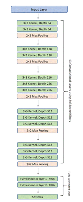
It consists of 16 layers, 13 of them being convolutional layers and 3 of them being fully connected layers (much lower compared to DenseNet’s 121 and ResNet’s 50 layers) along with 138 million different parameters¹⁵. The architecture is given in figure 4.

Unsupervised Model Architecture:

Unsupervised learning models are types of machine learning models that analyze data without labeled or predefined categories. Clustering models are a subset of unsupervised learning models that group or “cluster” unlabelled data. One such unsupervised learning model is K-means Clustering, which I chose due to literature precedence. K-means clustering is an iterative process to minimize the sum of euclidean distances between the data points (pixels for images) and their cluster centroids¹⁶. The distance can be calculated through the formula:

   

Methodology Overview

Through the two datasets, I developed 4 sets of supervised and unsupervised learning models: Supervised CNN models trained on dataset 1, supervised CNN models trained on dataset 2 , unsupervised K-means Clustering model trained on dataset 1 and unsupervised K-means Clustering model trained on dataset 2. I evaluated their effectiveness in classifying and clustering ocular diseases present within a fundus image.

Methods 

Datasets Used

The first dataset used was the Ocular Disease Intelligent Recognition (ODIR) structured ophthalmic database in Kaggle consisting of 3,196 left and right (in total, 6392) fundus images taken from the Shanggong Medical Technology Co. Ltd¹⁷. This dataset includes the fundus images of patients from different hospitals and medical centers all throughout China. The dataset was labelled by trained ophthalmologists with quality control management. It includes eight classes: Normal, Myopia, Diabetes, Glaucoma, Cataract, Age Related Macular Degeneration, Hypertension, Pathological Myopia and Other diseases and abnormalities. In this dataset, 2873 images were normal, 1608 contained Diabetic retinopathy, 284 contained Glaucoma, 293 contained Cataract, 266 contained Age Related Macular Degeneration, 128 contained Hypertension, 232 contained Myopia and 708 contained Other diseases. The “other diseases and abnormalities” class includes certain smaller abnormalities present within the eye that do not belong to one specific disease. Drusen, Atrophy and laser spots have been included in this class.

The second dataset used was the “eye_disease_classification” structured ophthalmic database in Kaggle. The dataset comprises fundus images taken from different sources including IDRiD, Ocular Recognition and HRIF. It includes 4,217 fundus images consisting of 4 categories: Normal, Glaucoma, Diabetic Retinopathy and Cataract. Diabetic Retinopathy consisted of 1098 images, Normal images with 1074, Cataract with 1038 images and Glaucoma with 1007 images.

Regarding the fundus images themselves, they are of slightly different color and resolution due to the difference in cameras used to take the images. This provides a good variety of images, which may help the quality of training data.

Data Cleaning & Balancing

For the supervised CNN models, I was able to use the maximum resolution of the fundus images (512×512). However, I chose 224×224 resolution while running the unsupervised K-means clustering model due to the following reasons:

● I needed the workflow to be less computationally expensive

● Before running the K-means clustering model, I did transfer learning by taking pre-trained weights from the ResNet50 architecture trained on imagenet. Most imagenet pre-trained models are trained on 224×224 RGB images and thus their convolutional filters and fully connected layers expect this resolution

I conducted normalization on each fundus image by converting the regular pixel scale (0 to 256) into a scale from 0 to 1 by dividing each pixel value by 255. This helps to reduce data redundancy and may improve model performance.

First Dataset:

After downloading, extracting and uploading the first dataset on my system, I was presented with both a single folder titled “preprocessed_images” containing all 6392 images and a CSV file with all the information for every image. In order to maintain subject-level splitting (both left and right eyes from the same patient should be in the same dataset), I first grouped each left and right eye image together and separated the dataset into 70% for training and 30% for testing. Furthermore, I took 80% of the training data for true training and 20% for validation. Afterwards, I sorted each image into their respective classes. Thus, I had 3577 images for training, 894 images for validation and 1921 images for testing.

In terms of training data, I had 1617 images for Normal, 399 images for Other, 124 images for Myopia, 75 images for Hypertension, 156 images for Age Related Macular Degeneration, 158 images for Cataract, 896 images for Diabetes and 164 images for Glaucoma.

In order to balance the training dataset (there is no need to balance the validation and testing dataset as they need to reflect a real-world distribution of classes), I employed both oversampling (artificially increasing the number of images of every class till it reaches the number of images in the class with the maximum number of images) and data augmentation (altering each image in order to differentiate them from their original image) till each class reached 1617 images. I allowed the following parameters to be changed in data augmentation:

● Rotation range = 20 degrees

● Width shift range = 0.1%

● Height shift range = 0.1%

● Shear range = 0.1%

● Zoom range = 0.1%

● Allowed horizontal flips

● Employed a “nearest” fill algorithm (empty pixels left when the image is altered should be assigned the value of the nearest pixel)

After running the algorithms, I had 1617 images for each training class. Therefore, here are the total number of images per class for training, validation and testing:

● Normal: 1617 training images, 404 validation images, 852 testing images

● Glaucoma: 1617 training images, 40 validation images, 80 testing images

● Cataract: 1617 training images, 39 validation images, 96 testing images

● Myopia: 1617 training images, 30 validation images, 78 testing images

● Hypertension: 1617 training images, 18 validation images, 35 testing images

● Diabetes: 1617 training images, 223 validation images, 489 testing images

● Age Related Macular Degeneration: 1617 training images, 39 validation images, 71 testing images

● Other: 1617 training images, 99 validation images, 210 testing images

 Second Dataset:

The second dataset contained 4,217 fundus images categorized in four classes: Normal, Cataract, Diabetes and Glaucoma. After following the same steps as I did for the first dataset, I ultimately had 601 images for Normal, 581 images for Cataract, 615 images for Diabetes and 564 images for Glaucoma. Employing the same balancing algorithm, I balanced all training classes to have 615 images. Therefore, the total number of images per class for training, validation and testing are as follows:

● Normal: 615 training images, 150 validation images, 323 testing images

● Glaucoma: 615 training images, 140 validation images, 303 testing images

● Diabetes: 615 training images, 153 validation images, 330 testing images

● Cataract: 615 training images, 145 validation images, 312 testing images

Unsupervised Learning:

In order to prepare the data for the unsupervised learning model (which does not require the data to be split into training at testing), I simply sorted and moved all of the preprocessed images from both datasets into their respective classes. However, I did not load the data based on classes and therefore maintained the unlabelled data needed for unsupervised learning.

Model Fine-Tuning

On loading the three Convolutional Neural Network models, I employed specific hyperparameter changes to maximize results. I ultimately chose 128 neurons in the Dense layer (after testing against resource and time constraints). Moreover, I chose 0.5 as the dropout rate (drops 50% of neurons during training) to ensure the absence of overfitting (dropout rates of 0.2 and 0.3 were tested but ultimately led to worse results). Furthermore, I chose ReLU as the hidden activation layer and Softmax as the output activation layer. In the K-Means clustering model, I set the number of clusters (k) to be equal to the number of disease classes for both datasets (8 for the first dataset and 4 for the second dataset).

Results

Supervised Evaluation Performance Metrics

I have included four of the most widely used model evaluation metrics for comparison: Accuracy, Precision, Recall and F1 Score. Moreover, I have calculated the Confidence Interval (CI) and ROC/PR-AUC as well.

Accuracy:

Accuracy is a supervised learning performance metric that is the proportion of all classifications that were correct and hence is defined as correct classifications/total classifications¹.

   

Micro-accuracy and Macro-accuracy are specific types of accuracy. Micro accuracy calculates the average by treating the entire dataset as an aggregate result. Macro- accuracy is defined as the average of the accuracy of each individual disease (in this study, the accuracy of each individual disease is taken with respect to the Normal class). Macro-accuracy is useful in unbalanced datasets as it provides accuracy in an unbiased form.

Precision:

Precision gives a clear view of how many positive-meaning disease patients are identified correctly among the entire dataset. Note that here, precision is calculated with respect to the Normal class¹.

   

Precision is used to determine how often the model predicts a certain disease when there actually is nothing.

Recall:

Recall, or true positive rate, is a supervised learning performance metric. It is the proportion of all actual positives (True Positives) and is defined as only True Positives/(True Positives + False Negatives). Note that here, recall is calculated with respect to the Normal class¹.

Recall is used to determine how often the model predicts that a fundus image does not contain a particular disease when it in fact does.

F1 Score:

F1 Score is defined as the harmonic mean of precision and recall. It gives equal priority to both¹.

Confidence Interval:

The confidence interval is a range of values that contains the true value. One type of confidence interval is the Wilson Confidence Interval, which is what I have used in this study. It is given by the following equation¹⁸:

   

Where,

● n is the total number of predictions

● p is the accuracy of the predictions (total number of correct predictions/n)

● z is a constant based on the percentage confidence interval (for 95% CI, it is 1.96)

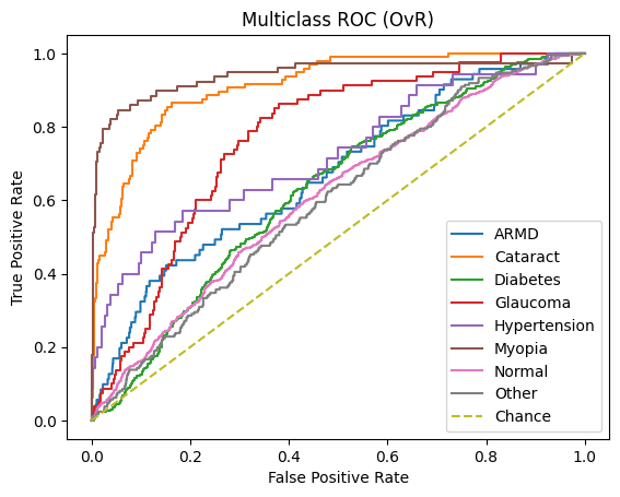
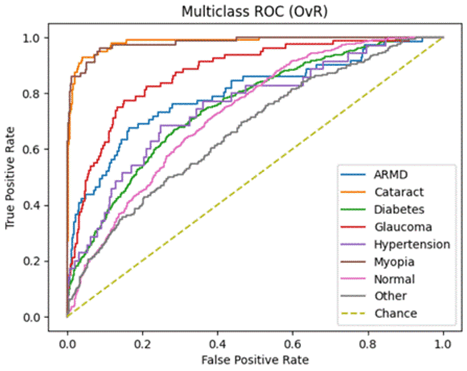
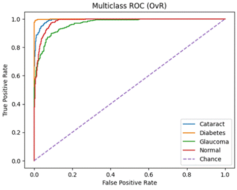
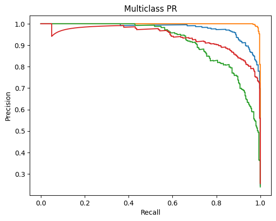
Receiver Operating Characteristics (ROC) and Precision-Recall (PR) – Area Under the Curve (AUC) [ROC-AUC and PR-AUC]:

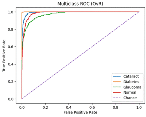
An ROC curve is a graph used to check how well a classification model works by plotting the True Positive Rate against the False Positive Rate.It first randomly chooses a pair (one from the positive class and one from the negative class) and checks whether the positive point has a higher predicted probability. Then it repeats this for all possible pairs.

The ROC-AUC measures the area under the ROC curve. It measures on a scale from zero to one where zero means that the model struggles to differentiate between the two classes (in this study, Normal vs all other diseases) and one means that the model can effectively distinguish between positive and negative instances.

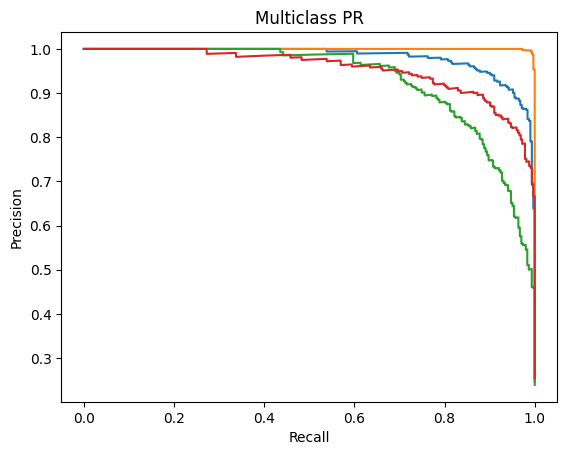
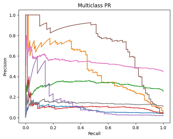
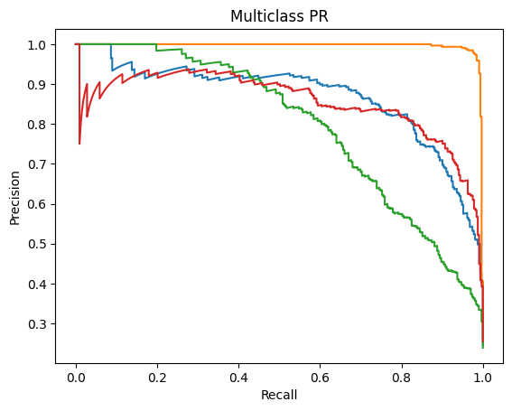
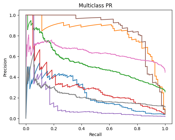
Precision-Recall Curve is a graphical representation (x-axis is Recall and y-axis is Precision) that represents how well a classification model is doing. It is especially useful when the data is imbalanced. The PR-AUC scale is also measured from zero to one (zero being a weaker classification model and one being a stronger classification model)¹⁹.

Unsupervised Evaluation Performance Metrics

Adjusted Random Index:

Adjusted Random Index (ARI) is an evaluation metric I have used to evaluate the unsupervised learning model K-means Clustering. In order to understand its mathematical definition, we must first define Random Index. The Random Index (Rand-Index) is an evaluation metric for clustering algorithms that provides a single score indicating the proportion of agreements between the two clusters. It is calculated by:

   

Where:

● ‘a’ represents the count of element pairs that belong to the same cluster in both methods

● ‘b’ denotes the number of element pairs assigned to different clusters in both approaches

● ‘n’ stands for the overall number of elements being clustered (here it is n/2 as it signifies the total count of element pars in the dataset)

ARI is a variation of Rand Index that adjusts for chance when evaluating the similarity between two clusterings. It is defined by¹⁷ :

   

Where:

● R is the Rand Index

● E is the expected value of the Rand index

● Max(R) is the maximum achievable value of Rand Index (always 1)

Normalized Mutual Information:

Normalized Mutual Information (NMI) is another popular metric for clustering evaluation and also quantifies the similarity between two clusters by scaling the mutual information to the range of 0 to 1. It is derived from Mutual Information (MI) which is a symmetric measure that quantifies the mutual dependence between two random variables. Normalized Mutual Information (NMI) is a normalized version of MI and is mathematically defined as¹⁷:

   

Where:

●  is the between the two partitions

●  and are the entropy values

Supervised Learning Model Results

The following are the results in terms of Accuracy, Precision, Recall and F1 Score obtained for the three models: ResNet50, DenseNet121 and VGG16 on the testing dataset.

Testing Accuracy (Micro):

	ResNet50	DenseNet121	VGG16
Dataset 1 (Unbalanced & 8 Classes)	55.73% (95% CI: 53.49% – 57.94%)	46.10% (95% CI: 43.88% – 48.34%)	54.95% (95% CI: 52.71% – 57.16%)
Dataset 2 (Balanced & 4 Classes)	90.77% (95% CI: 89.05% – 92.25%)	81.70% (95% CI: 79.48% – 83.73%)	89.35% (95% CI: 87.54% – 90.93%)

Testing Accuracy (Macro):

	ResNet50	DenseNet121	VGG16
Dataset 1 (Unbalanced & 8 Classes)	39.36% (95% CI: 36.81% – 41.91%)	27.39% (95% CI: 25.27% – 29.51%)	45.74% (95% CI: 42.69% – 48.79%)
Dataset 2 (Balanced & 4 Classes)	90.57% (95% CI: 88.99 – 92.16)	81.33% (95% CI: 79.29 – 83.38%)	89.13% (95% CI: 87.45% – 90.81%)

Testing Precision:

	ResNet50	DenseNet121	VGG16
Dataset 1 (Unbalanced & 8 Classes)	61.21%	63.72%	60.31%
Dataset 2 (Balanced & 4 Classes)	91.53%	84.16%	89.83%

Testing Recall:

	ResNet50	DenseNet121	VGG16
Dataset 1 (Unbalanced & 8 Classes)	47.31%	10.57%	38.25%
Dataset 2 (Balanced & 4 Classes)	90.38%	79.18%	89.20%

Testing F1 Score:

	ResNet50	DenseNet121	VGG16
Dataset 1 (Unbalanced & 8 Classes)	53.37%	18.13%	46.81%
Dataset 2 (Balanced & 4 Classes)	90.95%	81.59%	89.51%

Class-wise Testing Metrics:

ResNet50

Dataset 1:

Class	Accuracy (95% CI)	Precision (95% CI)	Recall (95% CI)	F1 Score (95% CI)
ARMD	21.1% (13.2–32.0%)	48.4% (32.0–65.2%)	21.1% (13.2–32.0%)	29.3% (17.4–48.9%)
Cataract	79.2% (70.0–86.1%)	76.8% (67.5–84.0%)	79.2% (70.0–86.1%)	77.9% (71.2–84.2%)
Diabetes	20.2% (16.9–24.0%)	66.4% (52.7–67.5%)	20.2% (16.9–24.0%)	30.3% (25.7–34.6%)
Glaucoma	8.7% (4.3–17.0%)	28.0% (14.3–47.6%)	8.7% (4.3–17.0%)	13.1% (4.5–22.8%)
Hypertension	11.4% (4.5–26.0%)	19.0% (7.7–40.0%)	11.4% (4.5–26.0%)	14.1% (3.4–27.3%)
Myopia	76.9% (66.4–84.9%)	87.0% (77.0–93.0%)	76.9% (66.4–84.9%)	81.4% (74.3–88.1%)
Normal	93.4% (91.6–94.9%)	54.3% (51.7–56.8%)	93.4% (91.6–94.9%)	68.6% (66.5–70.8%)
Other	3.8% (1.9–7.3%)	22.9% (12.1–39.0%)	3.8% (1.9–7.3%)	6.4% (2.4–11.8%)

Dataset 2:

Class	Accuracy (95% CI)	Precision (95% CI)	Recall (95% CI)	F1 Score (95% CI)
Cataract	91.0% (87.3–93.7%)	93.7% (90.4–95.9%)	91.0% (87.3–93.7%)	92.3% (90.2–94.4%)
Diabetes	97.0% (94.5–98.3%)	100.0% (98.8–100.0%)	97.0% (94.5–98.3%)	98.4% (97.4–99.4%)
Glaucoma	79.9% (75.0–84.0%)	87.7% (83.3–91.0%)	79.9% (75.0–84.0%)	83.5% (80.2–86.8%)
Normal	94.4% (91.4–96.4%)	82.7% (78.5–86.2%)	94.4% (91.4–96.4%)	88.1% (85.6–90.6%)

DenseNet121

Dataset 1:

Class	Accuracy (95% CI)	Precision (95% CI)	Recall (95% CI)	F1 Score (95% CI)
ARMD	9.9% (4.9–19.0%)	20.6% (10.3–36.8%)	9.9% (4.9–19.0%)	13.1% (4.5–22.2%)
Cataract	44.8% (35.2–54.7%)	40.2% (31.4–49.7%)	44.8% (35.2–54.7%)	42.1% (33.3–50.7%)
Diabetes	3.5% (2.2–5.5%)	28.3% (18.5–40.8%)	3.5% (2.2–5.5%)	6.1% (3.5–9.0%)
Glaucoma	5.0% (2.0–12.2%)	16.7% (6.7–35.9%)	5.0% (2.0–12.2%)	7.6% (1.8–15.1%)
Hypertension	0.0% (0.0–9.9%)	0.0% (0.0–79.3%)	0.0% (0.0–9.9%)	0.0% (0.0–0.0%)
Myopia	66.7% (55.6–76.1%)	71.2% (60.0–80.3%)	66.7% (55.6–76.1%)	68.7% (59.7–76.9%)
Normal	88.8% (86.6–99.8%)	47.3% (44.8–49.7%)	88.8% (86.6–99.8%)	61.7% (59.5–64.0%)
Other	0.5% (0.1–2.6%)	9.1% (1.6–37.7%)	0.5% (0.1–2.6%)	0.9% (0.0–2.8%)

Dataset 2:

Class	Accuracy (95% CI)	Precision (95% CI)	Recall (95% CI)	F1 Score (95% CI)
Cataract	84.3% (79.8–87.9%)	77.1% (72.4–81.3%)	84.3% (79.8–87.9%)	80.6% (77.1–83.8%)
Diabetes	91.2% (87.7–93.8%)	99.3% (97.6–99.8%)	91.2% (87.7–93.8%)	95.1% (93.2–96.7%)
Glaucoma	59.7% (54.1–65.1%)	78.0% (72.3–82.9%)	59.7% (54.1–65.1%)	67.7% (63.0–72.1%)
Normal	90.1% (86.3–92.9%)	74.2% (69.7–78.3%)	90.1% (86.3–92.9%)	81.4% (78.2–84.6%)

VGG16

Dataset 1:

Class	Accuracy (95% CI)	Precision (95% CI)	Recall (95% CI)	F1 Score (95% CI)
ARMD	22.5% (14.4–33.5%)	47.1% (31.5–63.3%)	22.5% (14.4–33.5%)	30.3% (18.9–41.4%)
Cataract	76.0% (66.6–83.5%)	78.5% (69.1–85.6%)	76.0% (66.6–83.5%)	77.0% (70.1–83.1%)
Diabetes	46.2% (41.8–50.6%)	53.2% (48.4–57.9%)	46.2% (41.8–50.6%)	49.4% (45.2–53.3%)
Glaucoma	40.0% (30.0–51.0%)	31.1% (22.9–40.6%)	40.0% (30.0–51.0%)	34.9% (26.3–43.8%)
Hypertension	17.1% (8.1–32.7%)	33.3% (16.3–56.3%)	17.1% (8.1–32.7%)	22.4% (7.4–38.5%)
Myopia	73.1% (62.3–81.7%)	83.8% (73.3–90.7%)	73.1% (62.3–81.7%)	77.9% (69.7–85.0%)
Normal	70.0% (65.8–72.9%)	59.4% (56.3–62.4%)	70.0% (65.8–72.9%)	64.2% (61.8–66.7%)
Other	21.0% (16.0–27.0%)	26.5% (20.4–33.7%)	21.0% (16.0–27.0%)	23.3% (17.7–29.1%)

Dataset 2:

Class	Accuracy (95% CI)	Precision (95% CI)	Recall (95% CI)	F1 Score (95% CI)
Cataract	90.1% (86.2–92.9%)	92.4% (88.9–94.9%)	90.1% (86.2–92.9%)	91.2% (88.9–93.4%)
Diabetes	97.9% (95.7–99.0%)	99.1% (97.3–99.7%)	97.9% (95.7–99.0%)	98.5% (97.4–99.3%)
Glaucoma	77.6% (72.5–81.9%)	82.5% (77.6–86.4%)	77.6% (72.5–81.9%)	79.9% (76.4–83.3%)
Normal	91.0% (87.4–93.7%)	83.3% (79.0–86.8%)	91.0% (87.4–93.7%)	86.9% (84.3–89.4%)

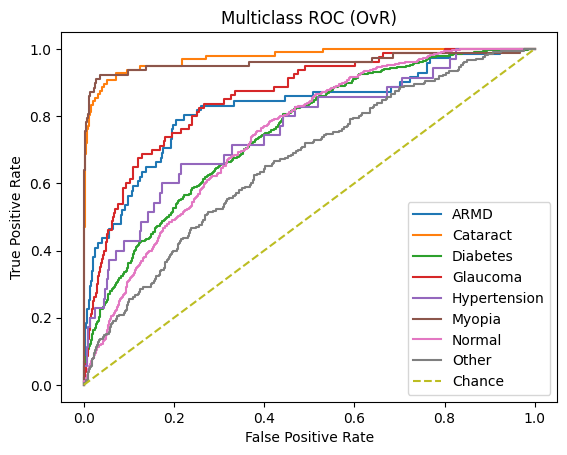
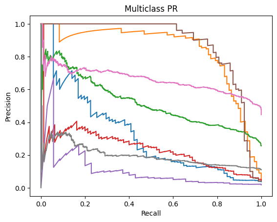
ROC-AUC and PR-AUC:

ResNet50

Dataset 1:

Class	ROC-AUC	PR-AUC
ARMD	0.823	0.323
Cataract	0.974	0.839
Diabetes	0.752	0.519
Glaucoma	0.856	0.243
Hypertension	0.757	0.113
Myopia	0.960	0.878
Normal	0.743	0.659
Other	0.662	0.196

Micro ROC-AUC = 0.904 | Macro ROC-AUC = 0.816

Micro PR-AUC = 0.596 | Macro PR-AUC = 0.471

Dataset 2:

Class	ROC-AUC	PR-AUC
Cataract	0.994	0.981
Diabetes	1.000	1.000
Glaucoma	0.972	0.931
Normal	0.985	0.954

Micro ROC-AUC = 0.991 | Macro ROC-AUC = 0.988

Micro PR-AUC = 0.974  | Macro PR-AUC = 0.966

DenseNet121

Dataset 1:

Class	ROC-AUC	PR-AUC
ARMD	0.671	0.082
Cataract	0.912	0.478
Diabetes	0.628	0.322
Glaucoma	0.768	0.115
Hypertension	0.724	0.141
Myopia	0.942	0.723
Normal	0.610	0.538
Other	0.598	0.142

Micro ROC-AUC = 0.860 | Macro ROC-AUC = 0.732

Micro PR-AUC = 0.463 | Macro PR-AUC = 0.318

Dataset 2:

Class	ROC-AUC	PR-AUC
Cataract	0.956	0.870
Diabetes	0.998	0.996
Glaucoma	0.902	0.796
Normal	0.957	0.856

Micro ROC-AUC = 0.962 | Macro ROC-AUC = 0.953

Micro PR-AUC = 0.904 | Macro PR-AUC = 0.880

VGG16

Dataset 1:

Class	ROC-AUC	PR-AUC
ARMD	0.797	0.241
Cataract	0.982	0.824
Diabetes	0.751	0.530
Glaucoma	0.873	0.309
Hypertension	0.752	0.146
Myopia	0.981	0.863
Normal	0.727	0.639
Other	0.667	0.217

Micro ROC-AUC = 0.899 | Macro ROC-AUC = 0.816

Micro PR-AUC = 0.564 | Macro PR-AUC = 0.471

Dataset 2:

Class	ROC-AUC	PR-AUC
Cataract	0.993	0.979
Diabetes	1.000	0.999
Glaucoma	0.966	0.918
Normal	0.982	0.940

Micro ROC-AUC = 0.989 | Macro ROC-AUC = 0.985

Micro PR-AUC = 0.971 | Macro PR-AUC = 0.959

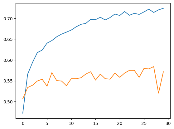
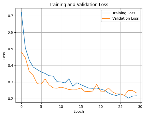
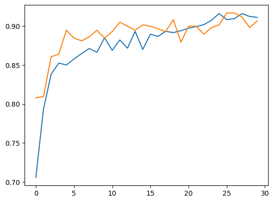
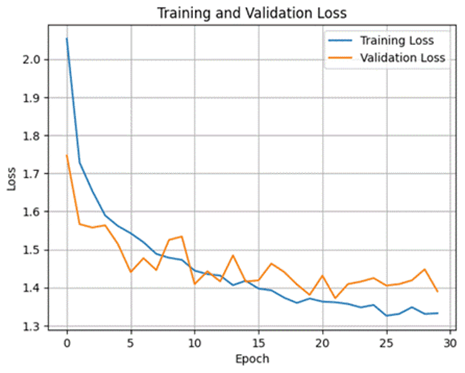
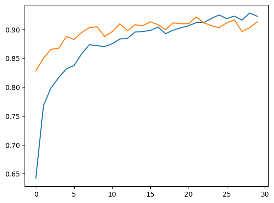
Accuracy, Training and Validation Loss Graphs:

ResNet50

Dataset 1

Dataset 2

DenseNet121

 Dataset 1

Dataset 2

VGG16

Dataset 1

Dataset 2

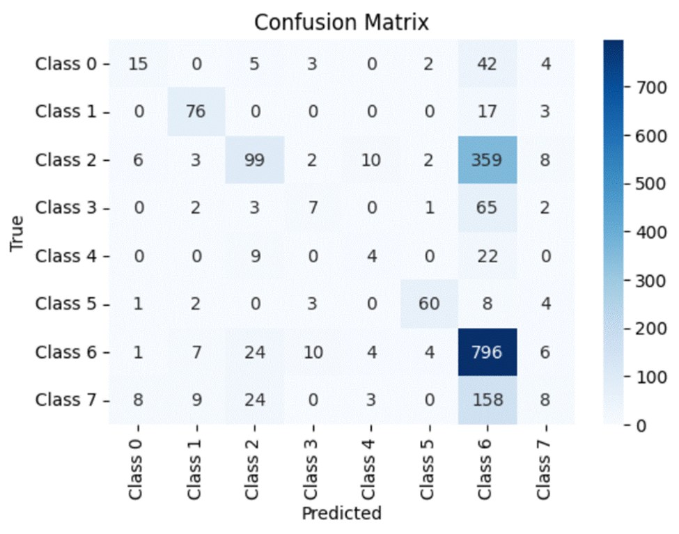
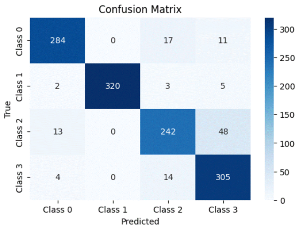
Confusion Matrices:

A confusion matrix is a simple and elegant way of visually evaluating how well a particular model is doing. It compares the model’s prediction (in this case, the horizontal axis) to the actual true value (the vertical axis). Thus for every value in the testing dataset, the value in the grid formed by the model’s prediction and the actual class the value belongs to will be incremented by 1. Ideally, a perfect model will predict every dataset value correctly and thus will have all of its values lying on the diagonal of the matrix.

Note that for the confusion matrix for Dataset 1:

1. Class 0 – Age Related Macular Degeneration
2. Class 1 – Cataract
3. Class 2 – Diabetes
4. Class 3 – Glaucoma
5. Class 4 – Hypertension
6. Class 5 – Myopia
7. Class 6 – Normal
8. Class 7 – Other Diseases/Abnormalities

Similarly, for Dataset 2:

1. Class 0 – Cataract
2. Class 1 – Diabetes
3. Class 2 – Glaucoma
4. Class 3 – Normal

ResNet50

Dataset 1

Dataset 2

DenseNet121

Dataset 1

Dataset 2

VGG16

Dataset 1

Dataset 2

Unsupervised Learning Model Results

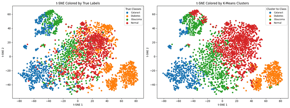
Here are the results of the unsupervised learning model K-means clustering trained on both datasets. Moreover, I have included the t-SNE Coloured labels (clusters predicted by the model) vs the true cluster label graphs.

Dataset 1

Adjusted Rand Index	0.0366
NMI	0.1145

Dataset 2

Adjusted Rand Index	0.3237
NMI	0.4118

Discussion

It is important to remember the differences between the two datasets before making interpretations. The first dataset consists of 8 different classes and thus would allude to, on average, 12.5% accuracy by random guessing. The second dataset only consists of 4 different classes, alluding to 25% accuracy by average guessing. Moreover, although the models were trained on balanced training data from both datasets, the testing dataset of dataset one is unbalanced. Therefore, while evaluating the models’ results on dataset 1, it’s more important to look at recall and micro/macro averages rather than each individual disease’s accuracy.

Supervised Learning Discussion

Let’s begin by systematically comparing all three models in accuracy, precision, recall and F1 score along with analyzing each model’s confusion matrix.

Evaluation Metrics Discussion:

By analyzing the micro accuracy for all three models, we can clearly see that ResNet50 has a slightly higher micro accuracy compared to VGG16 for both datasets. Moreover, both models outshine DensNet121 which has a significantly lower micro accuracy. When analyzing macro accuracy, both ResNet50 and VGG16 yet again significantly outperform DenseNet121. However, for the first dataset, VGG16 has a sizable lead in accuracy (around 6%), but ResNet50 does have a slightly higher macro accuracy for the second dataset. When discussing the precision and recall scores of each model, we can see that all three models have significantly better scores for the first dataset and slightly higher scores for the second dataset. Moreover, DenseNet121’s recall score is extremely low (less than, on average, 32% compared to ResNet50 and VGG16). A low recall score can be extremely dangerous when deployed in the healthcare field as the model may predict the absence of a disease, when in fact, that disease is present. From the F1 score, we can see that ResNet50 has a higher score compared to VGG16.

A similar story can be found when analyzing the micro/macro ROC-AUC and PR-AUC values. Both ResNet50 and VGG16 outperform DenseNet121. For the first dataset, ResNet50 has a slightly higher Micro ROC-AUC and PR-AUC and identical Macro values. ResNet50 slightly outperforms VGG16 in the second dataset as well.

To summarize, we can say that:ResNet50 and VGG16 significantly outperform DenseNet121 when evaluated on a real-world class distribution and still outperform the model when evaluated on a balanced dataset

● ResNet50 has overall the best results, slightly outperforming VGG16 in both datasets, except for the Macro accuracy in dataset 1

Confusion Matrix and Class-wise Discussion:

Note that the accuracy of each individual disease mentioned in this section stems from the following formula:

Accuracy of model X in predicting disease Y = (total number of images containing Y correctly predicted by model X)/total number of images containing Y taken for testing.

The total number of images containing Y taken for testing can be identified by adding the total number of images along the Y’s row in the confusion matrix. Moreover, the total number of images containing Y correctly predicted by model X can be identified by the number present in the grid where the Y’s row and Y’s column meet.

Through the analysis of the confusion matrices and metrics for each individual class for the first dataset, we can clearly see that all three models consistently maintain high accuracy, precision, recall and f1 scores for Normal images. Moreover, although the number of images present within the Myopia and Cataract classes were roughly equal and far less than those in the Normal and Diabetes classes, all three models also have high accuracy, precision, recall and f1 scores for those classes as well. However, all three models struggle with classifying the other diseases, particularly the Hypertension and “Other” categories. One interesting observation is that the ROC-AUC for the Normal class is on par with the other classes and only Myopia and Cataract have ROC-AUC scores above 0.9.

While analyzing the class-wise results for the second dataset, we can see that ResNet50 continues to maintain a slightly higher accuracy, precision, recall and f1 score for all four diseases. While looking at the results for Diabetes, we can see that VGG16 has a slightly higher accuracy and recall score (97.9% vs 97% for both classes) compared to ResNet50 but the latter has a slightly higher precision score (100% vs 99.1%). However, all three models struggle with classifying Glaucomatous eyes when compared to the other diseases. Therefore to conclude, we can say that overall, ResNet50 tends to be the most robust model over both datasets with VGG16 close by. DenseNet121 consistently lags behind the other two models.

Unsupervised Learning Discussion

The Adjusted Rand Index (ARI) is a numerical value that measures the similarity between the two assignments and the Normalized Mutual Information (NMI) estimates the clustering quality. Due to the low Adjusted Rand Index (0.0366) and low NMI (0.1145), one can say that the K-Means Clustering model cannot accurately cluster the unbalanced first dataset. Moreover, by analyzing the t-SNE Colored K-Means Clusters graph, one can note that the model is only able to identify Normal and Cataract images, failing to cluster the rest. In the second dataset, the model has achieved an Adjusted Rand Index of 0.3237 and an NMI of 0.4118. Furthermore, through the t-SNE Coloured K-Means Clusters graph, one can note that the model has been able to distinguish and roughly cluster the four ocular diseases.

Therefore, we can say that the K-Means clustering model cannot be satisfactorily applied to the larger first dataset (with an imbalance in testing data). In the smaller and balanced second dataset, the model is able to identify each disease, but cannot accurately distinguish between them.

Limitations and Future Work

This research was subject to limitations due to constraints on data acquisition and resources available to train the models. The use of two datasets which are already balanced (and do not need to be balanced artificially) will certainly improve model results. Furthermore, with even more specific hyperparameterized optimization and more fine-tune data cleaning, results of both the supervised and unsupervised learning models can be improved. The focus of this paper was to analyze and evaluate each model’s overall prediction ability. Fine-tuning and comparing each model for specific disease detection can also be studied.

Future studies should include training and evaluating Convolutional Neural Network models on more diverse datasets consisting of more categories of diseases. The inclusion and comparison of other supervised learning models such as Random Forest and Decision Trees can also be used. Moreover, the use of Hierarchical, Density-based, Distribution-based and Fuzzy Clustering models can be included to diversify the unsupervised learning part of this study. Finally, the use of semi-supervised learning approaches in classification and clustering can be explored.

Conclusion

In conclusion, the results acquired from the research conducted in this study, along with future work in the classification and clustering of ocular diseases present within fundus images, have the capacity to revolutionize ocular disease detection. The knowledge that ResNet50 was the most robust model out of all three in overall predictions can be essential towards deploying the right models to the right patients. Moreover, the results from K-means clustering can catalyze further research towards integrating unsupervised learning models in the healthcare industry–saving time-consuming work. Future research should prioritize training these models on larger and more robust datasets, along with the inclusion of non-CNN based models such as Decision Trees and Random Forests. Furthermore, future research in unsupervised clustering of ocular diseases should consist of hyperparameterized models that have been trained on more fine-tuned data.

Github Repository

Github Repository: https://github.com/PradhyumnaPrakash/Ocular-Disease-Classification-and-Clustering-

References

1. S. Ejaz, H.U. Zia, F. Majeed, U. Shafique, S.C. Altamiranda, V. Lipari, I. Ashraf (2025). Fundus image classification using feature concatenation for early diagnosis of retinal disease. Digital Health, 11. https://doi.org/10.1177/20552076251328120 [↩] [↩] [↩] [↩] [↩] [↩] [↩] [↩] [↩] [↩]
2. S. Chakraborty, A. Roy, P. Pramanik, D. Valenkova, R. Sarkar. A Dual Attention-aided DenseNet-121 for Classification of Glaucoma from Fundus Images. (n.d.). https://arxiv.org/html/2406.15113v1 [↩]
3. Y. Pan, J. Liu, Y. Cai, X. Yang, Z. Zhang, H. Long, K. Zhao, X. Yu, C. Zeng, J.. Duan, P. Xiao, J. Li, F. Cai, X. Yang, Z. Tan. (2023). Fundus image classification using Inception V3 and ResNet-50 for the early diagnostics of fundus diseases. Frontiers in Physiology, 14. https://doi.org/10.3389/fphys.2023.1126780 [↩] [↩] [↩]
4. Y. Jeong, Y. J Hong, J. H Han. Review of Machine Learning Applications Using Retinal Fundus Images. (2022, January). ResearchGate. https://www.researchgate.net/publication/357652601_Review_of_Machine_Learning_Applications_Using_Retinal_Fundus_Images [↩]
5. C. A. Briceno, MD. (2024, November 7). Nearsightedness: What is myopia? American Academy of Ophthalmology. https://www.aao.org/eye-health/diseases/myopia-nearsightedness [↩]
6. K. Allison, D. Patel, O. Alabi.  (2020c). Epidemiology of Glaucoma: the Past, Present, and Predictions for the Future. Cureus. https://doi.org/10.7759/cureus.11686 [↩]
7. M.V Cicinelli, J.C Buchan, M Nicholson, V. Varadaraj, R.C. Khanna. Cataracts. (2023). ScienceDirect. https://www.sciencedirect.com/science/article/abs/pii/S0140673622018396 [↩]
8. N. Salimiaghdam, M. Riazi-Esfahani, P.S. Fukuhara, K. Schneider, M.C. Kenney. (2019). Age-related Macular Degeneration (AMD): A Review on its Epidemiology and Risk Factors. The Open Ophthalmology Journal, 13(1), 90–99. https://doi.org/10.2174/1874364101913010090 [↩]
9. A. Bajwa, N. Nosheen,  K.I. Talpur, S. Akram. (2023). A Prospective Study on Diabetic Retinopathy Detection Based on Modify Convolutional Neural Network Using Fundus Images at Sindh Institute of Ophthalmology & Visual Sciences. Diagnostics, 13(3), 393. https://doi.org/10.3390/diagnostics13030393 [↩]
10. G. Liew, J. Xie, H. Nguyen, L.  Keay, M.K. Ikram, K. McGeechan, B EK. Klein, J.J.Wang, P. Mitchell, C CW.Klaver, E L. Lamoureux, T Y. Wong. Hypertensive retinopathy and cardiovascular disease risk: 6 population-based cohorts meta-analysis. (2023, June). ScienceDirect. https://www.sciencedirect.com/science/article/pii/S2772487523000132 [↩]
11. R. Yamashita, M. Nishio, R.K Gian, DO, K. Togashi (2018). Convolutional neural networks: an overview and application in radiology. Insights Into Imaging, 9(4), 611–629. https://doi.org/10.1007/s13244-018-0639-9 [↩]
12. N.K. Tyagi (2024). Implementing Inception v3, VGG-16 and VGG-19 Architectures of CNN for Medicinal Plant leaves Identification and Disease Detection. Journal of Electrical Systems, 20(7s), 2380–2388. https://doi.org/10.52783/jes.3989 [↩]
13. G. Huang, Z. Liu,  V.D.M. Laurens, & K.Q. Weinberger. (2016, August 25). Densely connected convolutional networks. arXiv.org. https://arxiv.org/abs/1608.06993 [↩]
14. P.K Mannepalli, V.D.S Baghela, A. Agrawal, P. Johri, S.S Dubey, K. Parmar. Transfer Learning for Automated Classification of Eye Disease in Fundus Images from Pretrained Model. (2024). International Information and Engineering Technology Association, 41(5). [↩]
15. S. Tammina. Transfer learning using VGG-16 with Deep Convolutional Neural Network for Classifying Images. (2019, October). ResearchGate. https://www.researchgate.net/publication/337105858_Transfer_learning_using_VGG 16_with_Deep_Convolutional_Neural_Network_for_Classifying_Images [↩] [↩]
16. A.M Ikotun, A.E Ezugwu, L. Abualigah, B. Abualigah, J. Hemang. K-means clustering algorithms: A comprehensive review, variants analysis, and advances in the era of big data. (2022). ScienceDirect. https://www.sciencedirect.com/science/article/abs/pii/S0020025522014633 [↩]
17. T. Zhang, L. Zhong, B. Yuan. A Critical Note on the Evaluation of Clustering Algorithms. (n.d.). Association for the Advancement of Artificial Intelligence. https://arxiv.org/pdf/1908.03782 [↩] [↩] [↩]
18. S. Wallis. Binomial Confidence Intervals and Contingency Tests: Mathematical Fundamentals and the Evaluation of Alternative Methods. (2007). ResearchGate. https://www.researchgate.net/publication/263683046_Binomial_Confidence_Intervals_and_Contingency_Tests_Mathematical_Fundamentals_and_the_Evaluation_of_Alternative_Methods [↩]
19. E. Richardson, R. Trevizani, J.A. Greenbaum, H. Carter, M. Nielsen, B. Peters.  (2024b). The receiver operating characteristic curve accurately assesses imbalanced datasets. Patterns, 5(6), 100994. https://doi.org/10.1016/j.patter.2024.100994 [↩]