Identifying Current Position of a Player Using Machine Learning Approach

Abstract

This research attempts to answer the question of whether machine learning can predict the position of a footballer based on commonly tracked statistics. Various statistics were input to the model and various versions of the dataset were created to build the optimal machine learning model. Through this preliminary analysis, averaged player statistics for each player over the course of an entire season was determined to be the best dataset with which to train the model. After additional hyperparameter tuning, we created a model that accurately predicted player position at an average rate of 72%. This relatively low percentage informs the conclusion of this study: It is difficult to identify a definitive statistical profile for any football position, likely due to the fluidity and flexibility of game play. However, the model’s accuracy does vary by position. The model is able to identify center backs at a rate closer to 85% of the time. By contrast, the wing position, which may involve more creativity and adaptability, was predicted at a rate much closer to 50%. These results highlight the complex and dynamic nature of positions in football and the difficulties of creating a statistical model to define a player’s position.

Keywords: football, season, match, player, position, EDA, machine learning, feature importance, SHAP

Introduction

 In football, each team starts with eleven players on the field. Each player is assigned a position with vastly different responsibilities. The amalgamation of all eleven players’ positions is called a formation. Formations usually have a balance of defence, midfield, and attack, but this can be changed if the team wants to emphasize one of the three phases of the game.

In football, the players are mobile, moving to make tackles, passes, and other small actions, but the overall shape of the formation tends to hold. Most teams have a different shape for when they have the ball and when they do not, although these shapes have to be somewhat similar to each other, as the players need to be able to react quickly if the ball is turned over and transition from their offensive shape to their defensive shape and vice versa. Within each section of these sections of the formation, there are different positions. For example, the attack is composed of the forward, who is the central attacker, and two wings who are the wide attackers. A “DM” refers to a defensive-minded midfielder who operates slightly higher up the pitch than the defenders, while an “AM” is an attack-minded midfielder who operates slightly behind the attacking players. These are just a few of the many possible positions. Occasionally, a team will include a very specific position in its formation that serves a much more focused purpose. An example of this would be a “false nine,” an attacking player who would lurk closely behind a forward and have much creative freedom. Within this framework, each player has a very specific job, and doing that job is integral to maintaining the purpose of the formation. For example, if the DM does not sit in front of the defensive line providing cover for the defenders, then the defenders have to step higher up the field, leaving more space behind them. If the winger does not maintain a wide position, then the fullback has nobody to pass to in order to advance the ball up the field. If a player is deployed in the wrong position within the formation, their particular skill set risks being wasted. Every player knows that they must do the job they have been told to do, so if a player is placed in a defensive position, they will defend – whether they are good at defending or not – as it is essential to the success of the team. However, this means that their possible offensive output will not be maximized, as they are not in the best field position to utilize their skills. Take, for example, a fullback. A fullback is the wide defender in the formation. Their job defensively is to defend the opposing team’s winger, and their job offensively is to support their own team’s winger in creating offensive chances for the forward or even for themselves. As part of this offensive job, sometimes a fullback ends up very high on the pitch in their attempt to contribute to a goal. But the second the ball is turned over, the fullback now has to chase the opposing team’s winger who will most likely be unmarked because of the fullback’s focus on offense. In this scenario, the fullback may be blamed as the cause for the opposing winger being left unmarked. This poses a very important question in this topic: If a player has been placed in the wrong position relative to his skillset, why can’t the coach or fans see it so clearly? The answer is that players do their best to fulfill the position they are assigned, performing the duties of the position, whether or not that is their best and highest use on the pitch.

In studying this topic of positions and evaluating how to find the positions for players with particular skill sets, there is a need to understand the relationships and connections between the duties and responsibilities of each position, while also challenging the way we view the sport. By examining closely the statistics that make a player successful at a particular position and exploring which players playing other positions had similar skill sets, it may become possible to evaluate each player’s attributes and evaluate whether they are more suited to play a different position. Lastly, if the model consistently confuses two positions, that may serve as evidence that there are concrete similarities between the two positions.

Extensive research has been conducted in recent years using data analytics to predict the position of a footballer. The study A Machine Learning Model to Predict Player’s Positions based on Performance by Zixue Zeng and Bingyu Pan (2021) used a handful of statistics and a machine learning model to predict position at an accuracy of 77%. The model used BP neural networks for the training. They also used hyperparameter tuning to find the best model, using parameters such as training rate and iterations. This study used, among other metrics, shot accuracy, passing accuracy, the accuracy of ground loose balls, accuracy of defending duel, and accuracy of air duel.

Plakias et al., (2023) conducted a systematic review related to identifying soccer players’ playing styles. They attempted to understand and quantify playing styles and positions to help aid coaches and organizations in maximizing the impact of their players. They concluded in their study that their framework for describing playing styles was applicable and accurate but acknowledged that more research would be needed to fully exploit their framework.

In contrast to other recent studies, our study seeks to understand how players’ positions interrelate, and whether the position for any player is identifiable from that player’s statistics, performance, and observable skill set. We propose to use machine learning techniques to build a model to identify the position for any given player given the player’s statistics, performance and observable skill set. Additionally, we seek to understand and quantify the effect of different statistics on model performance and accuracy.

Dataset

Our dataset contains every player’s performance in the English Premier League in the 2021-2022 season¹. The English Premier League is considered one of the most competitive professional Football leagues in the world. From that period, we examined every match, every player that played in that match, and their statistics from that match. The Premier League has 20 teams and the regular season consists of 38 games. Each team fields 11 players per game plus substitutions. This dataset yields 10,486 rows and 54 columns. Each row represents a player by name, and the rows corresponding to that column reflect each players’ statistics in one particular match, arrayed across 54 metrics.

It is important to acknowledge the limitations of the dataset used for this study. The sole dataset used to provide game statistics was a Premier League specific dataset, and only provided games from the 2021-2022 season. First, only including the Premier League is a limitation, as each league provides different playstyles². Only training in the Premier League could leave the model unprepared to assess La Liga, Serie A, Ligue 1, and Bundesliga Players. Furthermore, the inclusion of these leagues would provide a larger sample size. By training solely on the Premier League in this study, we opened up the limitation of not knowing whether the model performs beyond that very specific scope.

The second limitation of our dataset was that it only included one season. Football is an evolving sport where tactics, players, and coaches constantly change³. For example, the following season of this dataset was the highest scoring Premier League ever, until it was broken the following year. More goals can be likely attributed to more offensive tactics, which would in turn change the general statistics of every position. This is a great example of how the concept and patterns explored in this study may be outdated when evaluating current players (or any players outside of the 2021-2022 season).

Each of the 54 metrics (columns) relates to the player’s actions on the pitch, with the exception of columns that denote, for example, the number the player wears, the player’s nationality, position, and age. The remaining statistics measure player performance, some defensive, some attacking, and other statistics that apply to all positions like minutes played, successful duels and actions (offensive and defensive), and touches. Touches refers to every time the player touches the ball but only counts one touch before the ball is played to someone else. For example, if a player receives the ball, dribbles the ball, then passes the ball, the player would be counted as having one touch.

The attacking statistics include goals, assists, penalties/penalties attempted, shots, shots on target, attacking actions, and expected statistics. Expected statistics include expected goals, expected assists, and non-penalty expected goals. Expected statistics are often considered an advanced stat as they require much more complex calculation. These statistics measure a player’s execution relative to the opportunity presented in a game. For example, every time a player shoots the ball, statisticians calculate based on distance and angle relative to the goal how likely a shot is to score, on a range of 0-1 (closer to one means a higher likeliness of scoring). This statistical measure reflects the expected possibility of a goal in a particular situation (FIFA Training Centre). The expected goals of all of the player’s shots is then summed to determine the total expected goals of the player. The next column is non-penalty expected goals, which calculates the player’s expected goals minus any expected goals that were added in from a penalty kick. This is because a penalty kick opportunity is calculated as exactly 0.79 expected goal, and if a player takes a lot of penalties, their expected goals number would become inflated. Much like expected goals, expected assists is the calculation of how likely a player was to get an assist. The next attacking column is shot creating actions. This stat refers to the final two offensive actions that lead to a shot. This can include many different actions but most commonly passing (open play or a set piece) and dribbling. The next column is goal creating actions which tracks the shot creating actions that ended in a goal.

The Premier League also tracks a multitude of defensive/off ball statistics. These measures include statistics for infractions like the number of yellow cards and red cards the player was given in the match, but also includes positive defensive statistics such as tackles, which is defined as when a player completes a defensive action on an opposing player successfully taking the ball from them. Interceptions is the next of this category followed by blocks, which includes blocking passes and shots.

The final two categories are dribbling and passing statistics. Passing statistics are passes completed, followed by passes attempted. These statistics are both used to make the next column which is pass completion percentage (passes completed divided by passes attempted). The last passing statistic is progressive passes. A pass is defined as progressive, when the ball must travel towards the opposition’s goal. The first stat in the dribbling category is carries, which is when a player dribbles the ball for five meters. The last column is progressive carries which is carries in the direction of the opposition’s goal. The last 22 columns are goalkeeper-specific statistics which were disregarded in the analysis of this dataset.

Exploratory Data Analysis

This section explores the relationships between different statistics, as well as the relationship between specific positions and certain statistics. The graphs represent the average of each statistic  per position, per game. These figures are representative of the Premier League as a whole, and do not represent individual players. Because the goal of this section is to observe general patterns, it was deemed unnecessary to average each stat into per-90-minutes statistics. That said, normalization of the statistics could offer slightly more precise observations.

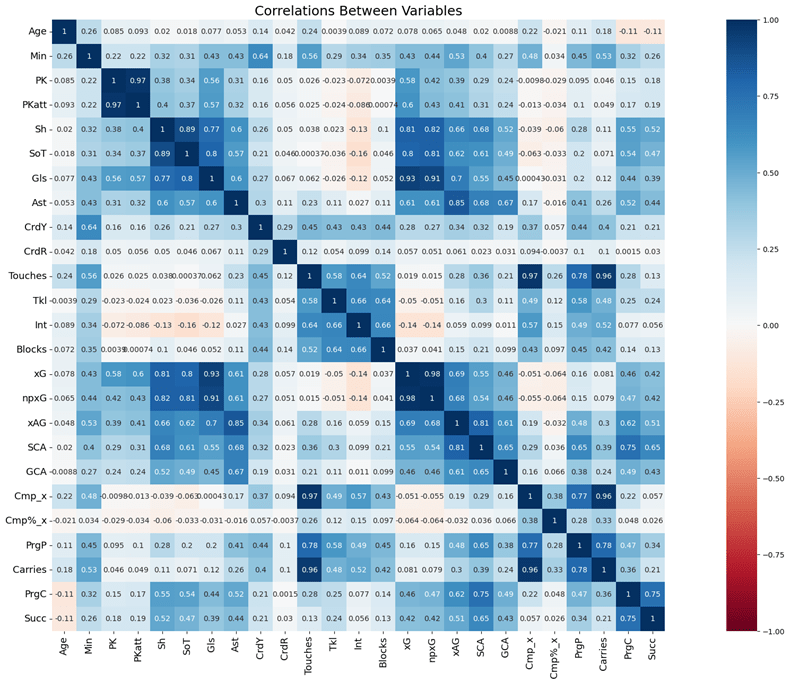
Figure 1 is a correlation matrix that displays the exact correlation between every variable in the dataset. Some variables have little to no correlation like penalty kicks and red cards. This makes sense as some statistics are simply not related. On the contrary, some statistics like xG and goals are extremely correlated (0.93) and can be explained logically. In this case the more expected goals a player has, the more goals they score. Another example of two correlated statistics is touches and carries. These two have a correlation coefficient of 0.96. This also can be explained logically, as the more times you receive the ball, the more often you dribble it for at least a few meters. It is important that there are statistics that are correlated as it makes it clear that there is collinearity in the dataset⁴.

The following figures are bar graphs using average statistics per position to understand patterns and relationships. Figure 2 shows the average progressive carries per match for each position. This plot can tell many stories and prompt many questions at a first glance. First, it is completely counter-intuitive that LW and RW would not be equal or at least close in progressive carries per match, yet LW is far above all the other positions in this statistical category. Second, Figure 2 also highlights how wide positions excel at progressive carries, with all wide players being above 1.5 progressive carries. The only non-wide position above 1.5 is AM.

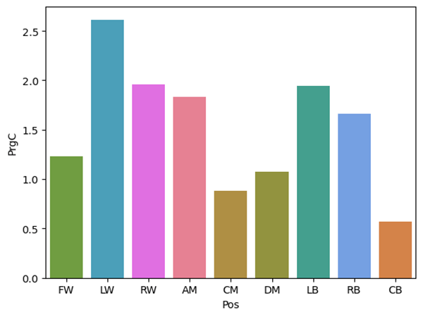
Figure 3 is another bar plot with positions on the X-axis, except this bar plot has minutes played on the y-axis. Figure 3 is especially intriguing, because it shows that some positions play fewer minutes per game, on average, than others. In particular, the data reflects that attacking positions play the fewest minutes. This raises many questions around whether some positions playing more minutes might skew or change the interpretation of their statistics. In basketball, statistics are often expressed as a function of every 100 possessions to ensure that players are evaluated on a basis that accounts for variations in minutes played per game. Considering the variation in minutes per game shown in figure 3, a system of normalization would be apt for evaluating statistics. However since the variation is not too drastic, this study will assume that the broader trends will still show when using per game metrics.

Figure 4 goes hand in hand with Figure 3. This is a bar graph of position and completed passes. Figure 4 shows that defenders complete the most passes, which could be explained by the fact that teams often pass the ball around their defensive area easily because opposing players are less concerned with breaking up passes in their opponent’s defensive end, far from their own goal. But could this graph be impacted by defenders’ increased minutes played relative to attacking players? This is an interesting idea to explore and could easily impact the interpretation of a graph like this one.

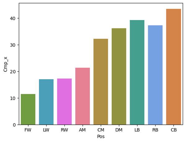
Figure 5 is a graph of expected goals by position. As expected, the more offensively-minded the position, the higher the expected goals. However, center backs present an exception to this expectation, as on average they accumulate slightly more expected goals than the fullbacks. A second intriguing nuance shown in Figure 5, is the almost equal expected goals that CM and DM accumulate. Their relationship becomes even more interesting when compared to the expected goals per game of AM, which is significantly above both.

Figure 6 is a plot of age and position. Age is not something that is often considered in an evaluation of a player’s style of play, and instead tends to be referenced more frequently in conversations around transfers and future potential. The five average youngest positions are LW, RW, AM, LB, and RB. Figure 2 explores averaged progressive carries per game, per position. In that figure, those same five positions average the most progressive carries per game. This creates an interesting correlation between player age and style, which could be explored in future research to decide whether this reflects causation.

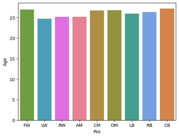
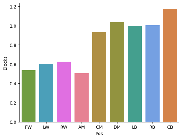
Figure 7 is an interesting plot, because in many ways it tells the story of the three midfield positions. The DM is the most defensive and accumulates even more blocks than fullbacks. The AM is the opposite, accumulating fewer blocks than any other position. The CM is often seen as the fulcrum between game phases, a balance of attacking and defending. But figure 7 shows that CM is actually closer to a DM than an AM. This can also be seen in the graph of expected goals, where CM and DM are right next to each other at ~0.05 xG, and AM is above that at ~0.15 xG.

Methods and Models

Input Features and Output Target

The machine learning model needs to be given input features so that it can learn the data and provide an output. The target output identifies the position of the player. The input features consist of the player statistics minus all goalkeeper statistics and any statistics that did not reflect or implicate the player’s ability on the field. The number the player wears was left out of the inputs alongside the nation. The 27 statistics used for the model were: Age, Min, PK, PKatt, Sh, SoT, Gls, Ast, CrdY, CrdR, Touches, Tkl, Int, Blocks, xG, npxG, xAG, SCA, GCA, Cmp_x, Cmp%_x, PrgP, Carries, PrgC, Succ, Pos, Att_x, as shown in Table 1. Ultimately, these statistics were chosen between a mix of domain expertise and simple reasoning. This study was not seeking to predict goalkeepers, as they have different, unique statistics. Given this, all goalkeeper statistics such as saves were removed. Following the goalkeeper statistics, all statistics that did not have any positional implication or performance implication were removed. This grouping only consists of the players nation, the players number, and whether the players team was home or away. Number was removed because many players pick numbers correlating to their position. For example, many defensive midfielders choose six, so much so that describing a player as a six has colloquially turned into a synonym for the position. Due to this correlation, it did not make sense based on the goal of this study to essentially give the model the output in certain scenarios. The reason the nation was removed is similar. If the model could spot trends between nations often fulfilling similar roles, this would say nothing about the qualities and relationships of the positions, but the identity and qualities of the nations themselves. The home or away stat was removed for the same reason, being that it says nothing about the position itself. Following the removal of the aforementioned statistics, there were 27 statistics left in the dataset that fit all the criteria to be given to the model. While these stats do encompass every position, the constraint of the dataset used for this study is important to acknowledge as a potential limitation. Statistics such as dribbles attempted, or pressures could have improved the success of this study.

Variable Name	Description
Age	Age of the player
Min	Minutes played
PK	Penalty Kick Goals
PKatt	Penalty Kicks Attempted
Sh	Shots
SoT	Shots on target
Gls	Goals scored
Ast	Assists
CrdY	Yellow cards
CrdR	Red cards
Touches	Touches of the ball
Tkl	Tackles
Int	Interception
Blocks	Blocked passes and shots
xG	Expected goals
npxG	Non penalty xG
xAG	Expected Assists
SCA	Shot creating actions
GCA	Goal creating actions
Cmp_x	Completed passes
Cmp%_x	Percentage of passes completed
PrgP	Progressive passes
Carries	Carries of the ball in any direction
PrgC	Progressive carries
Succ	Successful actions or duels
Att_x	Combination of attacking statistics to make a value
Pos	Position of the player

Output Target Pre-Processing

We preprocessed our target variable, position of the player, as shown in Table 2. First, all positions that were assigned to the left or right side of the pitch are combined to a new position that does not specify the side. This choice was made based on the assumption that the side of the pitch a player plays on would not impact their numerical statistics. We do not have access to information beyond the numbers, so footedness, style, and tendencies all had to be regarded as non-factors. Thus, our study does not include asymmetric tactics, but rather focused on the general position of a player. Moreover, left and right wingers serve the same role; There are right-footed left wingers and left-footed right wingers, same as there are left-footed left wingers and right-footed right wingers. Based on these evaluations of side designated positions, the choice to combine left and right sided positions seemed logical. This same thought process of symmetry was applied to other positions such as right back and left back. So, any right back or left back was revised to be described as a fullback, and any left or right winger was amended to be just a winger.

Second, in the original data some players played different positions in the same game. In this case all positions played would be listed. This offered a dilemma: if only one position is taken, then the data of that match will be skewed, as it is possible a player spent half of their minutes as an attacker and the other half as a defender. This would result in both high offensive statistics and high defensive statistics. Alternatively it is also impossible to predict that a player played two positions just by looking at the statistics, especially because such instances were relatively rare so that there was little data about these matches to learn from. Ultimately, in all games the only position used was the one  in which the player started, and then that position was modified according to the way that position was eventually transformed.

Third, originally there were 12 positions as shown in Table 2. Some positions did not have enough data points which resulted in significant data imbalance. To deal with data imbalance we proposed to group some of the positions together. Wingback is a position that is a slightly more offensive fullback. Since most teams use a formation with four defenders (two centre backs and two fullbacks) wing backs can be rare in the Premier League. To deal with this, wingbacks were lumped with the most similar position – fullback – as seen in Table 2. This means that all WB were described as FB to the model, and WB was no longer an option for the model to predict. This method was used for all positions that simply did not have enough data. For example, defensive midfield and attacking midfield had to be combined into a general midfield with central midfielders shown in Table 2.

Description	Original Position	Grouped Position
Defense, Center Back	CB	CB
Defense, Left Back	LB	FB
Defense, Right Back	RB
Defense, Wing Back	WB
Midfield, Defensive Midfielder	DM	M
Midfield, Central Midfielder	CM
Midfield, Attacking Midfielder	AM
Attack, Left Midfielder	LM	W
Attack, Right Midfielder	RM
Attack, Left Winger	LW
Attack, Right Winger	RW
Attack, Forward	FW	FW

Models and Evaluation Metrics

We split our dataset into training and test sets using a stratified split based on the proportion of the position labels with the test size of 20%. The details and strategies of this split are explained in the next section. Two baseline models, logistic regression⁵ and KNN⁶, were implemented for the sole purpose of comparison to our other models. These baseline models helped us understand what models were best at handling our data.

In addition to logistic regression and KNN, ensemble models such as Random Forest and XGBoost were implemented. Random Forest gets its name because it is the culmination of many decision trees⁷. Each tree uses random chunks of the data to make a prediction. The pros of using Random Forest are that in certain cases it mitigates overfitting and has a high accuracy. A con, however, is its ability to mitigate overfitting depends on the dataset. The next model after Random Forest, is Extreme Gradient Boosting or XGBoost⁸. XGBoost uses similar trees, but each tree builds upon the last to become more accurate upon the final prediction. Some pros of XGBoost include accuracy and speed. However, a significant con of XGBoost is overfitting.

            We used precision, recall, F1 score, and macro-averaged F1 to evaluate our models. Precision represents the percentage of the total guesses that were true. Recall is slightly different. Instead of comparing the true predicted center backs to the false predicted center backs, recall compares the true predicted center backs to the total center backs. Lastly, F1 score is the harmonic mean between precision and recall, giving a balanced score between the two ratios⁹.  Additionally, we used macro-averaged F1 to analyze our models more broadly. Macro-averaged F1 calculates the F1 score for each class independently, then averages these scores. This approach treats each class equally, regardless of the number of instances in each class. This metric provides a balanced evaluation of the model’s performance across all classes, making it useful for assessing performance in imbalanced datasets. All four of these metrics were used to address overfitting.

An important technique used to maximize the efficiency of the models was hyperparameter tuning. Hyperparameter tuning is essentially altering the model to find the best combination of settings for the model¹⁰. Random Forest and XGBoost have different parameters due to their different ways of functioning. To test the parameters, a grid search is used. What this means is that for each parameter a range is set depending on the parameter, and each possible model is tested and the grid search will identify the best one¹¹. The grid search has to run through every combination, so more parameters and larger ranges mean that the grid search will take longer. If the parameters are limited and the ranges cut down, this process can be very fast. Ultimately this process is very much trial and error.

There were four parameters tuned for Random Forest as shown in Table 3. “N_estimators” with the range being set to 100 and 500. “Min_samples_split” with the range being 30-150. “Max_features” with the range being 1-26. Lastly, “class_weight” was set to “balanced.” This setting helps address the issue of class imbalance in the dataset by automatically adjusting the weights assigned to each class. In practice, this means that the model places greater emphasis on correctly predicting instances from underrepresented classes, which would otherwise be overlooked due to their rarity. By rebalancing the contribution of each class to the overall loss during training, this parameter encourages the model to be more sensitive to minority class patterns, improving its ability to generalize across all classes.

The six parameters for XGBoost were tuned as shown in Table 3. First, “Eta,” with the range being set as 0.01, 0.05, 0.1, 0.2, and 0.3. The next parameter is “subsample,” having a range of 0.5, 0.6, 0.7, 0.8, and 0.9. The third parameter, “colsample_bynode,” has an identical range to “subsample.” “Gamma,” which was added to control overfitting, has a range of 0, 0.1, 0.2, 0.5, and 1. The last two parameters “Lambda” and “Alpha” have identical ranges of 0, 0.01, 0.1, 1, and 10. Additionally, the “scale_pos_weight” parameter was included to help address class imbalance by assigning more weight to the positive (minority) class. This parameter adjusts the gradient updates during training to account for skewed class distributions, making the model more sensitive to underrepresented classes. By increasing the relative importance of the minority class, it helps XGBoost avoid bias toward the majority class and improves performance in imbalanced classification settings.

Additionally, cross validation of the hyperparameter tuning was set to 3. This splits the dataset into three sections, so that the model can be tested to reduce overfitting¹². Another detail to note is that the F1 score for the tuned models was weighted. This was done to make up for the imbalanced distribution of position. This way, positions that had fewer players would still have an F1 score that accurately represents them.

Model	Parameter	Description	Range
Random Forest	n_estimators	Amount of trees	[100,500]
	max_features	Controls most features for splits	between 1 and 26 with increment of 1
	min_samples_split	Lowest number of samples required to split a node	between 30 and 150 with increment of 5
	class_weight	Balances class importance	“balanced”
XGBoost	eta	Learning rate	[0.01, 0.05, 0.1, 0.2, 0.3]
	subsample	Fraction of data for tree	[0.5, 0.6, 0.7, 0.8, 0.9]
	colsample_bytree	Fraction of features for tree	[0.5, 0.6, 0.7, 0.8, 0.9]
	gamma	Lowest loss reduction to split node	[0, 0.1, 0.2, 0.5, 1]
	alpha	L1 regularization	[0, 0.01, 0.1, 0.3, 0.5, 1]
	lambda	L2 regularization	[0, 0.01, 0.1, 0.3, 0.5, 1]
	scale_pos_weight	Control the balance of positive and negative weights	[1,10,50, 100]

Prediction Approaches: Match vs Season

There were two approaches chosen in the development of the models. First approach used a dataset using players by match. The second approach used a player’s season which took an aggregate of a player’s statistics across all of their matches. The result of this was a dataset consisting of one, more well-rounded, entry per player. The season dataset is, for the most part, averaged out and outlier performances in a single match can be mitigated by the rest of the performances. To create the “by season” dataset, each stat had to be either summed or averaged depending on the nature of the stat. Statistics like touches, where each player accrues many of them throughout a match, made sense to be averaged. Whereas a stat like goals, which are much more rare and even scarcer for non-attacking positions, made sense to be summed.

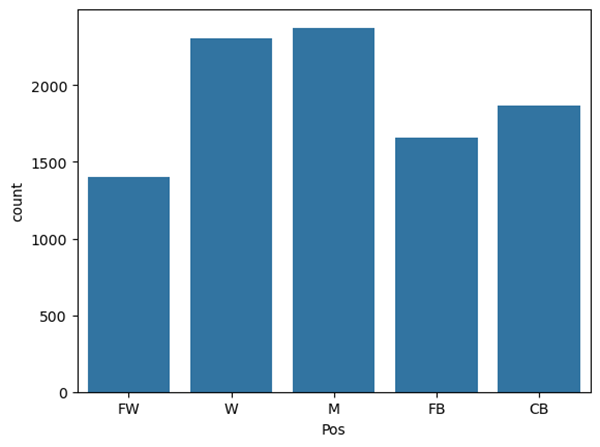
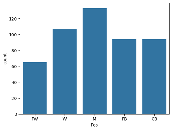
Figures 8 and 9 show the difference in the position distribution between the two datasets (by match and by season). Figure 8, the “by match” dataset, has at least 1000 player performances for each position to draw from. Also, W and M are the most common positions, which can be explained by the way the positions were lumped (table 2). In Figure 9, W and M are still the most common positions, but the amount of players per position has decreased significantly as there is only one entry per player. This distribution comparison between the original dataset (Figure 8) and the grouped one (Figure 9) can be described as mildly imbalanced. There are some slight changes in the shapes in Figure 9, but nothing major or worth concern.

We split “by season” and “by match” (Figure 8 and Figure 9) datasets into training and test sets using a stratified split based on the proportion of the position labels. The test dataset comprises 20% of the data. The “by season” dataset was simple to split, and therefore had zero data leakage.

The “by match” dataset had every match for each individual player, which made it more challenging to split into train and test sections. Controlling leakage in this dataset was particularly important, because if the model was able to train based on the statistics of one match from a player and then test on a different match from the same player, it could lead to deceptively high accuracy. All performances from each player were placed in either the test or the train, but never both. Although this new complication in the stratification made it harder to maintain balanced proportions of  positions, the final “by match” dataset was properly separated to avoid any leakage. Additionally, it is important to note that there was no overlap between the “by season” and “by match” datasets, and each was evaluated as a separate entity.

Results and Discussion

This section will discuss the results of the models and attempt to explain the reasons why each position performs the way it does. There are two different types of models used, and two different datasets that the models use. This section will be focusing on four models that have each been selected as the best model in its category. One Random Forest model and one XGBoost model were chosen for the by-match dataset. For the “by season” dataset, also one Random Forest and one XGBoost model has been selected. These four models will be compared to see which approach was more effective and why that is the case. Individual positions will also be compared, and the results of these positions will be explained using Football logic. Furthermore, the feature importance of the best performing model will be analyzed to strengthen the understanding of the models.

Results for Prediction of Player’s Position by Match

Table 4 represents the Logistic regression, KNN, Random Forest and XGBoost models after hyperparameter tuning for models using the “by match” dataset. These models were selected because that combination of parameters resulted in the highest F1 scores and limited overfitting.

In the Random Forest results, it is evident that the model is operating at around 50% for FB and FW. This is not a good result even for a model that has multiple outputs. Next, W and M are being predicted very inaccurately, sitting at F1 scores of 0.39 and 0.41, respectively. The only position that is being predicted with some success is CB, with an F1 score of 0.73. While 0.73 is not ideal, it is significantly better than all the other positions. The XGBoost model had very similar results, but is slightly more accurate in almost all sections. The positions that have the highest and lowest F1 scores stayed the same. CB still has the highest with a slightly improved 0.74. M still has the lowest at a much improved 0.44. But most interestingly the two positions that were sitting around an F1 score of 0.50 got slightly worse.

Model	Position	Precision	Recall	F1	Macro- Average F1	Sample Counts
Logistic regression	CB	0.67	0.81	0.73	0.54	427
	FB	0.54	0.5	0.52		342
	FW	0.49	0.69	0.57		322
	M	0.5	0.37	0.42		525
	W	0.49	0.43	0.46		465
KNN	CB	0.51	0.69	0.58	0.43	427
	FB	0.39	0.42	0.41		342
	FW	0.47	0.48	0.48		322
	M	0.34	0.28	0.31		525
	W	0.41	0.32	0.36		465
Random Forest Model class_weight: balanced, max_features: 5, min_samples_split: 30, n_estimators: 500, class_weighgt = “balanced”	CB	0.68	0.78	0.73	0.52	427
	FB	0.54	0.51	0.52		342
	FW	0.49	0.62	0.55		322
	M	0.45	0.34	0.39		525
	W	0.41	0.42	0.41		465
XGBoost Model eta: 0.01, subsample: 0.5 colsample_bytree: 0.9, gamma: 0 lambda: 1 alpha: 0	CB	0.71	0.78	0.74	0.54	427
	FB	0.58	0.45	0.51		342
	FW	0.59	0.48	0.53		322
	M	0.46	0.43	0.44		525
	W	0.41	0.52	0.46		465

Results for Prediction of Player’s Position by Season

Table 5 is the best Random Forest and XGBoost models after hyperparameter tuning for models using the “by season” dataset. The “by season” dataset only has one entry per player (as it is all of their matches statistics averaged/summed), so there are significantly fewer players for the model to pull from.

The Random Forest results in Table 5 are more accurate than the Random Forest in Table 4. This can be seen by the highest F1 score which is 0.87 for CB, but also through the increase in macro F1 which serves as a solid summary of how the model is performing. Overall, this model is performing decently with the lowest F1 scores ranging from 0.5-0.6. The XGBoost in Table 5 is an improved model over the Random Forest model in almost every category. The highest F1 is still CB with an unchanged 0.87, but M and FB improved to reach the 0.70 mark. Again, surprisingly one F1 score decreased, this time W, which went down to 0.49. Overall W performs very poorly across all models while CB performs very well, consistently staying above the overall averages. As noted in our methodology, the test set is drawn per season, which results in relatively small but relatively uniformly distributed class sizes across all positions as shown in Table 5. This design ensures fairness across roles, but also naturally limits the number of samples per class, including the FB class. Random Forest does not perform as well overall, especially when compared to XGBoost. As shown in Table 5, XGBoost demonstrates better consistency and generalization across classes, including the FB group.

Model	Position	Precision	Recall	F1	Macro- Average F1	Sample Counts
Logistic Regression	CB	0.79	1.00	0.88	0.69	19
	FB	0.8	0.63	0.71		19
	FW	0.65	0.85	0.73		13
	M	0.65	0.48	0.55		27
	W	0.57	0.62	0.59		21
KNN	CB	0.33	0.42	0.37	0.28	19
	FB	0.2	0.16	0.18		19
	FW	0.19	0.23	0.21		13
	M	0.33	0.3	0.31		27
	W	0.35	0.33	0.34		21
Random Forest Model max_features: 3, min_samples_split: 30, n_estimators: 500 class_weight : “balanced”	CB	0.85	0.89	0.87	0.67	19
	FB	1.00	0.47	0.64		19
	FW	0.67	0.77	0.71		13
	M	0.58	0.70	0.63		27
	W	0.50	0.52	0.51		21
xgBoost Model colsample_bynode: 0.5, eta: 0.1,  gamma: 0.5, subsample: 0.6	CB	0.85	0.89	0.87	0.72	19
	FB	1.00	0.63	0.77		19
	FW	0.69	0.85	0.76		13
	M	0.68	0.78	0.72		27
	W	0.50	0.48	0.49		21

Feature Importance Analysis

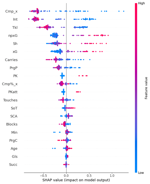
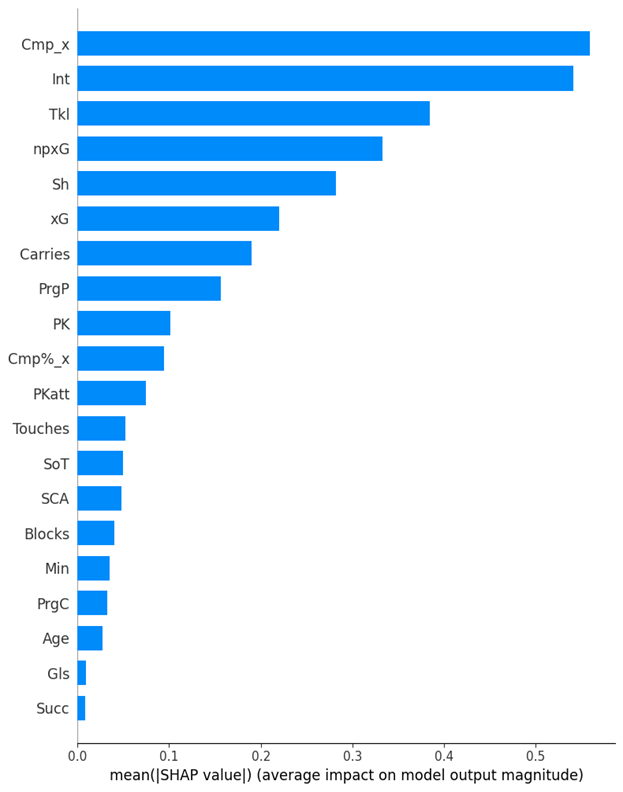
This section will analyze the individual impact of each feature on the best model’s ability to predict each position using TreeSHAP. The model that was deemed our best, was our XGBoost “by season” dataset model, which can be found in table 5. XGBoost supports an efficient, model-specific method called TreeSHAP, which computes exact Shapley values for tree-based models¹³. TreeSHAP is usually faster and more accurate for XGBoost compared to generic methods. Feature importance analysis is very useful to interpret the reasoning behind how the model is predicting each position. These figures explain which statistics were very important, and which ones were essentially useless.

Many of the features in this dataset are correlated, some more than others. This means the model treats these statistics as interchangeable because one offers no more value than the other in predicting the position of a player. When using SHAP, these statistics will not be labeled as having the same importance, even though they are interchangeable to the model. Instead, one statistic will be picked and the other discarded. However TreeSHAP will equally weigh the importance between correlated statistics. If regular SHAP was used, the SHAP analysis would be deemed unreliable due to the multicollinearity. But since TreeSHAP was used, the results can be analyzed due to the specific Tree-based qualities of TreeSHAP. Differently put, TreeSHAP understands correlation between variables, and thus accounts for it, enhancing the reliability of the SHAP analysis.

Figure 10 specifically explains which statistics had the greatest impact on the model’s ability to predict the position of players who were CB. A negative SHAP value indicates that the statistic made it harder for the model to predict that player and vice versa. Additionally, the color of the SHAP value indicates whether it was more or less of the stat that affected the model positively or negatively. At the top of the ranking by a large margin was SCA (shot creating actions). Figure 10 shows that when a CB has a high amount of SCA, the model is impacted negatively, which appears to signal that a CB who has high attacking statistics would be confused as an attacking player. The next statistic down the graph is touches. CBs accumulate many touches per game. When a CB has a lot of touches, that affects the model positively. But when a CB is not touching the ball often, the model is affected negatively. Interestingly, age was not the least impactful stat, even though anyone of any age can play a position. The figure shows that being older helped the model predict that a player was a CB.

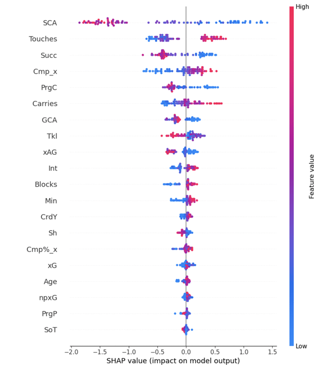
Figure 11 details that a high pass completion percentage is the most impactful statistic for the model to accurately predict a player as a midfielder. This can be explained by the way that midfielders are involved in all the stages of offense and complete high numbers of passes to progress the ball. Similarly, progressive passes are very impactful statistically and reflect the importance of midfielders in progressing the ball to the attacking players.

Figure 12 shows that when a FW makes many passes, tackles and interceptions, the model confuses the player for other positions. This makes sense, as the purpose of a FW is often only to impact play in the final third. Moreover, a FW having a high number for the majority of the statistics appears to throw the model off. This all could be due to the limited action most FWs get, where most of their involvement is simply to shoot and score in the final third. This can be seen in the SHAP values, where shots and expected goals being higher, allows the model to better predict a FW.

Discussion

Tables 4 and 5 maintain similar trends like CB having the highest F1 score, but the models represented in Table 5 are much more reliable. This can be seen in a simple cross check from the two tables. In Table 4, FW is middle of the pack in F1 at around 0.50. In Table 5, FW is again middle of the pack but at around 0.70. This improvement can be attributed to the “by season” dataset having much more rounded out entries. Although there are fewer entries, the “by season” dataset has by definition fewer outliers. The “by match” dataset’s struggles can be attributed to the unpredictable nature of a single match. If a CB scores three goals out of the 38 matches, the model will most likely be confused in the three matches in which the CB scored. However in the “by season” dataset, it is apparent to the model that the player scores at a very low rate of three goals a season and is therefore likely to be a defending player.

Also, which positions struggle to be predicted and which ones do not can be explained in part through the sport itself. CB was always the highest F1 score and this can be explained for two reasons. First, every formation includes two centre backs and some even three. So every roster contains around 4-5 CB in total that touch the field. This means that even in the “by season” dataset there were many entries. The second reason is that CB is a very defined position. Many positions have a multitude of play styles that can still be considered as the position. CB on the other hand has arguably only two roles in modern football. Some CBs are ball-playing defenders, who make many passes and even carry the ball upfield. Others are not, which simply means that their team/system has another way of moving the ball upfield and the CBs are not expected to be involved in the offensive buildup. It should also be said that in almost every circumstance defenders defend in the same ways. This creates little variety in their statistics and thus makes the position easiest to predict. Lastly, no other positions were combined into the CB category so it is composed of all center backs.

This logic can also be applied to the positions that were not resulting in accurate prediction, like W. The highest F1 scores in Tables 4 and 5 for W are 0.51 and 0.46 respectively. There are some identifiable reasons that may explain why W was not being predicted accurately. First, as discussed, all LM and RM players were combined with RW and LW players in the category W, making W the combination of four different positions. However, Wingers have many different playstyles. Some are inverted wingers, meaning they are left footed right wingers or vice versa. These wingers often attack by cutting toward the middle of the pitch to shoot. There are touchline wingers who gravitate to the wide part of the field and emphasize crossing the ball. There are inside wingers who play outside the FW but leave room down the sideline for the FB. As a result, unlike with CB, these variations in playstyle may confuse the model.

Additionally, while the dataset used for this research used many different players and games to provide a sufficient amount of data to examine, it is important to remember that this research used data from only one Premier league season. Football is an ever-evolving game, so drawing data from additional past years could provide new insights for future work. Similarly, there are hundreds of professional leagues all across the world which could provide additional depth in perspective.

Due to the collinearity throughout the statistics, feature engineering would be an effective strategy to simplify the data and improve the models. In future research, this can also be beneficial for the analysis of feature importance as removing the correlated features will remove redundancy.

When comparing the results of this study with the one by Zixue Zeng and Bingyu Pan (2021), “A Machine Learning Model to Predict Player’s Positions based on Performance,” it is clear that predicting the position of a footballer using machine learning is a difficult task. Zeng and Pan used neural networks to predict the position of footballers based on a wide range of statistics, similar to those used in this study. However, they also incorporated physical characteristics, such as height and weight, and used data from multiple seasons. In contrast, the models in this study only utilized match performance statistics like tackles or blocks, gathered from the collective performances of a single Premier League season.

Zeng and Pan argued that the inclusion of statistics like height could help predict the position of a player, because physical traits aid performance in certain positions such as height for goalkeeper or center back. That said, they concluded their best model to predict at 73%. In comparison, our best XGBoost had a macro F1 score of 0.72. Given the similarity of these numbers, it seems that physical traits may have had a minimal impact on the success of predicting the position of a player.

However, there is an important limitation to consider in our own research. In this study, only five broad position categories were predicted. Grouping improved the success of the model, while sacrificing specificity. Zeng and Pan on the other hand, predicted many distinct positions while still maintaining a 73% accuracy. While both models performed similarly, their methodology of neural networks, a broader dataset, no positional groupings, and physical traits appear to have yielded a greater classification accuracy.

Our position groupings were intentionally designed based on domain expertise and functional similarity among roles on the pitch¹⁴. For example, both Left Back (LB) and Right Back (RB) were grouped under Full Backs (FB), and central midfielders (DM, CM, AM) were grouped as Midfielders (M), reflecting common tactical groupings used in football analytics. Our grouping strategy was chosen to balance granularity with model interpretability and class balance. More fine-grained groupings, while potentially interesting, would have introduced substantial class imbalance and reduced the statistical reliability of the results—especially for rarer positions. We acknowledge that certain misclassifications may still occur within groups (e.g., between LM and LW), and examining confusion patterns across finer labels is indeed a promising direction. However, conducting a full statistical analysis of all possible grouping permutations is non-trivial and beyond the scope of this work. We consider this a valuable area for future research and will note this explicitly in the revised discussion.

Conclusions

The goal of this study was to understand and explore the best way to predict positions in Football. Many steps were taken in the path to reaching this goal, but ultimately there was one approach that stood out:  Using data that is averaged across a player’s entire season. This approach was more successful than the “by match” dataset, and out of the two models, XGBoost was more accurate than Random Forest. Additionally, more success was found when positions were combined, limiting the positions the Model was outputting.

After a process of elimination, the XGBoost “by season” model was found to be the most accurate model made in this research. Some rejected models could not predict positions at a rate better than 50%; these models used the “by match” dataset. The reason that the “by season” dataset succeeded where the “by match” failed is consistency. There were uniform trends among players that were spotted in the “by season” data that were corrupted by outliers in the “by match” data. To visualize this phenomenon, consider that the “by season” data represents the trend line, and the “by match” data shows every point, including every outlier.

In assessing the best model, the impact of features was dependent on the specific position. CBs had different feature importance than FWs. However, feature importance was not decided by how relevant the statistic was to the position. Instead it was both the most essential statistics and the least essential to a specific position. For CBs, an example of this phenomenon is that having high touches (essential) allows the model to predict CB. But having low shot creating actions (inessential) also allows the model to predict CB. This conclusion is drawn from the SHAP analysis; however it should be approached with caution as these features were heavily correlated. This means that two statistics, like goals and expected goals, were redundant to the models and thus one might have been labeled as unimportant when that conclusion is actually misleading. TreeSHAP was specifically used to mitigate this; however it is still possible that the correlation of statistics impacted the analysis.

The goal of this study was to see if machine learning could predict the position of footballers only by their performances. Using this study, coaches can find multiple ways to effectively improve their players. One use for this model is it could be used to predict and find alternate positions and or position changes. This model takes a player’s stats and guesses its most similar positions. Assuming that a player’s statistics are a good measurement of their skill sets, the model is essentially linking a player’s skill set to a position. A coach could use this to hone in on their players specific skills that play into the position the model assigns them. For example, if this model predicts a fullback as a centre back because of their passing statistics, a coach could move towards developing that player as a ball playing center back. Likewise, this model could be used to better understand how a player plays within their position. If a midfield player is predicted as a winger it is most likely that the midfielder has a more attacking mindset and skill set. A coach could use this information to allow that midfielder more leniency in joining the attack. This approach would not necessarily use a position change or alternate position, but rather a tactical shift to better utilize a player’s skill set. Additionally, if a new player is brought into a club, possibly through transfer or academy, it is useful information to know their possible positions. Therefore, using this model, a coach could know what position best suits a player before ever seeing their performance live.

In a future study, many strategies can be used to evolve this research. First, utilizing feature engineering to have more reliable SHAP to analyze would be an important step to better the understanding of feature impact. Second, drawing data from both multiple years and multiple leagues would be a great way to improve the data. Given the positive impact of using data that was averaged out from the Premier League, there would possibly also be a positive impact from averaging data from all over the world and past seasons. Third, in future research maintaining more positions without compromising accuracy would be ideal. As much as this research has been successful and interesting, a study that can explore the same ideas but predict more than five positions could be more enlightening to the nuances of positions. Lastly, with these future improvements in mind, applying this framework to other sports such as basketball could be an interesting way to compare different or similar results and trends between the two sports.

References

1. Orcan. Premier League – Game and Player statistics 2021-2024 (2024). https://www.kaggle.com/datasets/memocan/premier-league-games-and-player-stats-2021-2024 [↩]
2. Fernández, J., & Bornn, L. (2020). Wide open spaces: A statistical technique for measuring space creation in professional soccer. MIT Sloan Sports Analytics Conference. http://www.sloansportsconference.com/wp-content/uploads/2020/02/SSAC20_SSAC-Wide-Open-Spaces.pdf [↩]
3. Gama, J., Žliobaitė, I., Bifet, A., Pechenizkiy, M., & Bouchachia, A. (2014). A survey on concept drift adaptation. ACM Computing Surveys, 46(4), 44:1–44:37. https://doi.org/10.1145/2523813 [↩]
4. Dormann, C. F., Elith, J., Bacher, S., Buchmann, C., Carl, G., Carré, G., … & Lautenbach, S. (2013). Collinearity: A review of methods to deal with it and a simulation study evaluating their performance. Ecography, 36(1), 27–46. https://doi.org/10.1111/j.1600-0587.2012.07348.x [↩]
5. Hosmer, D. W., Lemeshow, S., & Sturdivant, R. X. (2013). Applied Logistic Regression (3rd ed.). Wiley. https://doi.org/10.1002/9781118548387 [↩]
6. Cover, T. M., & Hart, P. E. (1967). Nearest Neighbor Pattern Classification. IEEE Transactions on Information Theory, 13(1), 21–27. https://doi.org/10.1109/TIT.1967.1053964 [↩]
7. Breiman, L. Random Forests. Machine Learning 45, 5–32 (2001). https://doi.org/10.1023/A:1010933404324 [↩]
8. Chen, T. Guestrin, C. XGBoost: A Scalable Tree Boosting System (2016). https://arxiv.org/abs/1603.02754 [↩]
9. Sokolova, M., & Lapalme, G. (2009). A systematic analysis of performance measures for classification tasks. Information Processing & Management, 45(4), 427–437. https://doi.org/10.1016/j.ipm.2009.03.002 [↩]
10. Yu, T. Zhu, H. Hyper-Parameter Optimization: A Review of Algorithms and Applications (2020). https://arxiv.org/abs/2003.05689 [↩]
11. Shah, R. Tune Hyperparameters with GridSearchCV (2025). [↩]
12. Bergstra, J., & Bengio, Y. (2012). Random search for hyper-parameter optimization. Journal of Machine Learning Research, 13(Feb), 281–305. http://jmlr.org/papers/v13/bergstra12a.html [↩]
13. Lundberg, S. M., & Lee, S.-I. (2017). A Unified Approach to Interpreting Model Predictions. Advances in Neural Information Processing Systems,30. https://proceedings.neurips.cc/paper_files/paper/2017/file/8a20a8621978632d76c43dfd28b67767-Paper.pdf [↩]
14. Chmura, P., Konefał, M., Zając, T., Kowalczuk, E., & Andrzejewski, M. (2019). A new approach to the analysis of pitch-positions in professional soccer. Journal of Human Kinetics, 66(1), 143–153. https://pmc.ncbi.nlm.nih.gov/articles/PMC6458575/ [↩]