
Abstract
Housing markets are complex systems influenced by a variety of economic and demographic factors. This study evaluates several machine-learning models to analyze housing price trends in Mercer County, NJ, from 2012 to 2022, ultimately employing a neural network to predict future housing prices. This neural network attained an MAE of 31052, an RMSE of 46356, and an R² of 0.975. By integrating census data on median house value, median household income, racial composition, and educational attainment within Mercer County, this research explores spatial disparities in housing value across the region and reveals its correlations with other socioeconomic conditions. The findings reveal persistent economic inequality, with the Trenton area having significantly lower housing values and incomes and higher price volatility than regions such as Princeton across the entire span of data. The relevance of historical data in predicting real estate dynamics is shown by future forecasting, suggesting that these tendencies are likely to persist. In the context of housing market modeling, deep learning is crucial because it sheds light on the socioeconomic variables that influence housing disparities.
Keyword: Housing Inequality, Deep Learning, Neural Network, Mercer County, Housing Price Prediction, Socioeconomic Factors
Introduction
Housing markets are complex systems influenced by a variety of economic and demographic factors. Understanding housing price trends and the factors that influence outcomes is essential for addressing broader issues of affordability, economic stability, and inequality. Housing markets are highly localized and are influenced by regional economic conditions, demographics, and historical development patterns.
To improve prediction and understanding of housing market trends, this paper investigates the housing market of Mercer County, New Jersey. This county provides a compelling case study due to its stark contrasts between its northern and southern regions. The high home values and strong education in Princeton in the north make it one of the most desirable locations to live in the state. Trenton, on the other hand, has experienced decades of economic decline and housing instability despite its status as the state’s capital1.
This study employs machine-learning methods to analyze housing price trends in Mercer County, NJ, from 2012 to 2022, testing several models and ultimately constructing a neural network to predict future housing prices. By integrating census data from the American Community Survey (ACS) 5-Year Estimates on median house value, median household income, racial composition, and educational attainment within Mercer County, this research explores spatial disparities in housing value across the region and reveals its correlations with other socioeconomic conditions. The effectiveness of the models in forecasting future housing prices is assessed using an analysis of mean absolute error (MAE), root mean square error (RMSE), and R2 scores.
The remainder of this paper begins by reviewing prior research on housing prices, income, spatial characteristics, and the application of machine learning in real estate analysis. It then outlines the data sources, preprocessing, and models used to predict housing values. The results present geographic visualizations of economic and demographic characteristics in Mercer County and evaluate the model’s performance. The discussion interprets the socioeconomic insights and their implications for the housing market. Finally, the conclusion summarizes the findings and suggests directions for future research. Against this background, the central research question is: Can integrating socioeconomic variables into machine learning-based housing price forecasts provide new insights into spatial inequality and affordability trends?
Literature Review
The relationship between housing prices and key factors like income, spatial characteristics, and financial institutions has been a central focus of research, especially as housing affordability and inequality continue to be major global concerns. Housing markets are complex, with fluctuations in house prices often tied to broader economic shifts. However, these trends are not the same everywhere. Regional differences play a significant role in shaping housing dynamics, which means that understanding local economic conditions and demographic factors is crucial when examining housing prices. As these regional influences become more important, it’s clear that the way income distribution and local economies interact with housing prices is key to addressing issues like economic inequality and residential segregation.
Many works have examined the role of income in affecting house prices. Özmen and colleagues found a negative correlation between income and house prices in Turkey, in turn concluding that increases in income inequality reduced sensitivity of house prices to income changes2. Earlier studies conducted by Gallin and Chen and colleagues likewise explored the long-term relationship between house prices and income, finding limited evidence for cointegration but stronger short-term effects driven by monetary variables like money supply growth. These findings underscore the complexity of income and price dynamics, with economic features driving short-run volatility even in the absence of stable long-term relationships3,4.
Furthermore, a wide range of studies have consistently put forward the importance of analyzing regional trends and factors as a means of identifying correlations to housing prices rather than creating a single national housing market and policy to address the economy. Reichert showed that factors like population, employment, and permanent income affect housing markets differently across regions, even though certain national trends like mortgage rates continued to have uniform influences5. Similarly, Bruyne and Hove presented how relative geographical factors such as distance to important economic centers and availability of transportation greatly affect the value of such living spaces6. Locational attributes and amenities, in particular employment patterns, accessibility of transportation, school quality, and housing supply shocks, are key determinants of housing price volatility with respect to location7. These findings highlight the limitations of national economic models in explaining housing prices, emphasizing the need to account for regional variations in economic and spatial characteristics through localized analysis. The disproportional growth between GDP per capita and median household income as studied by Nolan and colleagues also attests to the importance of careful consideration of various indicators, with trends in the contributory factors of income growth measures often being dependent on the indicator chosen8.
In addition to these economic factors, financial and societal institutions also play a part in determining house prices. Steegmans and Hassink noted that the financial position of a household can affect bargaining power differences and consequently transaction outcomes9. Even considering the lack of exact specifications in defining the “middle class”10, greater differences in relative status between buyer and seller contributed to lower bargaining power. Tsatsaronis and Zhu found that inflation and interest rates were greatly tied to housing prices, with inflation and interest rates in countries creating strong feedbacks between credit growth and property prices11.
Environmental and infrastructure variables play a significant role as well. Hanna showed that pollution has income-dependent effects on housing values due to varied decision making at different income levels12, while Voith demonstrated that locations with greater access to transportation have higher prices, especially those in closer proximity to valuable commuter rail services13.
Predicting housing values has become a central focus in machine-learning research due to its importance for real estate markets, urban planning, and socioeconomic analysis. In this regard, economic and regional studies provide important insights on the impact of physical attributes on house price. However, while interpretable, past models often struggle with nonlinear relationships and complex interactions among variables.
More recent works have increasingly employed machine learning to capture these complex housing price dynamics. Tree-based methods such as Random Forest, Gradient Boosting Machines, and modern variants like XGBoost and LightGBM have shown strong predictive performance compared to traditional regression techniques due to their ability to handle nonlinear data and complex feature interactions. For instance, Sibindi and colleagues developed a hybrid ensemble model combining LightGBM and XGBoost, demonstrating that hybrid boosting models can outperform single-algorithm models by balancing variance and computational efficiency14. Even so, simpler tree-based methods also serve as strong baselines. Adetunji and colleagues applied a Random Forest regression to the Boston Housing dataset, predicting individual house values and demonstrating the viability of machine learning in handling detailed features and data15. A recent example of neural network-based house price prediction is presented by Wijaya, who evaluated complex relationships within the Boston Housing dataset by using a three-level dense neural network model16.
Beyond physical and locational factors, housing values have incorporated socioeconomic and behavioral features. Notably, Zhu and Sobolevsky have utilized digital records of social activity patterns like complaints and taxi trips to enhance modeling of house price levels and changes17. Zhao and colleagues have integrated other features, such as traffic and emotional cues, to analyze different characteristics and their relations to real estate values18. These efforts show that socioeconomic context can significantly enhance model accuracy and interpretability.
Nevertheless, a gap remains in the literature regarding deeper integration of socioeconomic features with machine-learning models, while geospatial analyses of housing markets often map observed prices rather than model-generated predictions of forecasted house values.
This study addresses these gaps by testing various machine-learning models and employing a neural network model that incorporates socioeconomic features, including household income, racial composition, and educational attainment. Using this model to predict housing values, this study links the predictions to geospatial mapping in order to identify broader trends and disparities. In doing so, the study extends prior machine-learning approaches by connecting predictive modeling with socioeconomic and spatial analysis.
Study Area
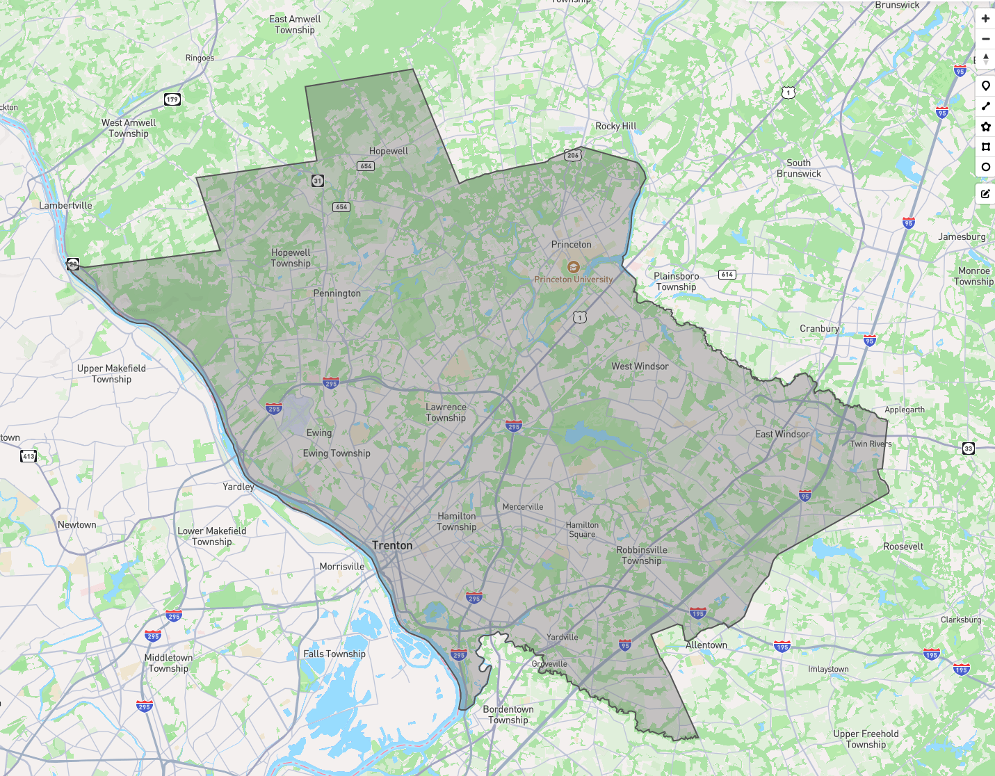
Figure 1. The Study Area: Mercer County, New Jersey
In Mercer County, Trenton has historically been a major industrial hub of iron, steel, rubber, and pottery throughout the 19th and 20th centuries19. However, as the city began its post-WWII deindustrialization in the 1950s, the economy entered a state of economic decline and widespread unemployment. The arrival of Black migrants was met with racist attitudes that fostered a relatively segregated urban landscape, especially within housing. Many white homeowners relocated to suburban areas like Princeton in order to escape the impoverished Trenton area, contributing to white flight and deepening the socioeconomic divide between Trenton and the rest of Mercer County that still persists today20.
In contrast to Trenton’s economic struggles, Princeton University in the northern part of the county has played a significant role in shaping Mercer County’s housing market. The high demand for housing from teachers and students alike has sharply increased the house values in the surrounding area, and the presence of an Ivy League institution and the highly ranked education system around Princeton has similarly made the region highly sought after1. These qualities have further exacerbated disparities in housing price growth and stability compared to economically disadvantaged urban Trenton.
A history of racial segregation through federal housing policies such as redlining reinforced the racial divisions of the time, limiting the opportunities for many minorities from accessing homes in other communities. Trenton was one such city, being both highly densely populated and filled with “obsolete” homes. With over half of the city’s metropolitan housing classified as hazardous or definitely declining, much of the community was redlined, significantly impacting the relative wealth of the region21. Understanding these historical and racial dynamics provides critical context for analyzing the housing price trends and socioeconomic inequalities examined in this study.
Method
Data Preprocessing and EDA
This study examines housing value, income, and racial composition trends across census tracts in Mercer County, NJ. All data used spans 2012 to 2022, inclusive, taken from the American Community Survey 5-Year Data provided by the U.S. Census Bureau. By analyzing median house values, median household income, racial composition, and educational attainment within the United States, this study seeks to explore patterns of housing inequality and economic disparities in the region.
One limitation in the data is that the United States TIGER boundaries are re-evaluated every ten years to better reflect changes in socioeconomic characteristics. As a result, including data from 2012 to 2022 results in two separate sets of geographic data: from 2012 to 2019, and from 2020 to 2022. For example, census tract 3301 was split into census tracts 3303 and 3304 in 2020, and consequently tract 3301 only has data from 2012 to 2019, while tracts 3303 and 3304 only contain data from 2020 onwards. In order to estimate the population values for these newly defined census tracts, the 2020 ratio between new tract values was applied to all the 2012-2019 values for the original tract. Values measured using median such as median house value, on the other hand, are copied from the original tract into both of the new tracts. From 2020 onwards, these new tracts retrieve their respective data. The rows for the original census tracts have been removed, since the data is contained within the two new census tracts and would otherwise be counted twice if left in the data. This preprocessing is a significant generalization of data within these tracts from 2012-2019, assuming that populations within these tracts are changing at fixed rates to one another and economic characteristics remain constant throughout the region. This is made more severe by the fact that census tracts are split to better encapsulate changing trends within these regions, meaning the socioeconomic qualities are anything but uniform. However, more specific data on these tracts is not available and ACS provides survey estimates rather than full counts, and such assumptions must be made to make use of these tracts.
Some data cells have a value of -666666666, indicating that the value was hidden for privacy reasons. These missing values are replaced using linear interpolation from the surrounding years, or forward fill and backward fill if the missing value is for the first or last year in range. Two census tracts consisted entirely of NA values and were consequently removed. Although these techniques were applied to handle missing values, it is important to note that these techniques may introduce bias by increasing the linearity of the data. Linear interpolation assumes a smooth transition between neighboring years, while forward and backward fill assume that previous or subsequent years have identical data. These assumptions may not reflect the true distribution of data and could impact the performance of predictive models, especially linear regression models, by underestimating the true variability. However, since the data represents a time series, smooth transitions can be expected between neighboring points, and linear interpolation is an appropriate method for filling in missing values. Furthermore, these gaps in the data are relatively small, and interpolating the data is still preferred to leaving these data points as NA or 0, which would introduce other distortions.
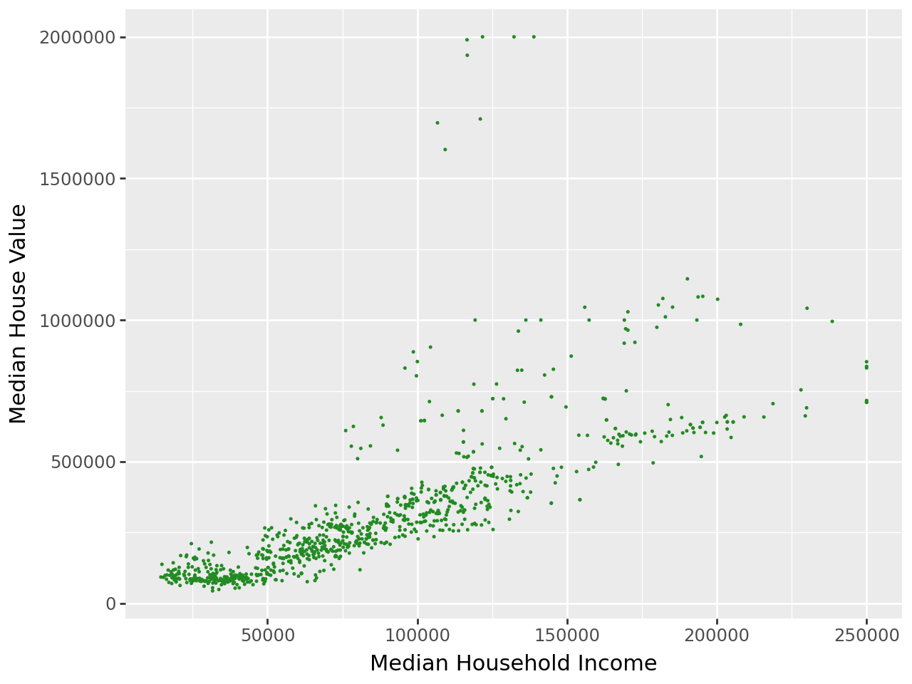
Figure 2. (a) Median household income

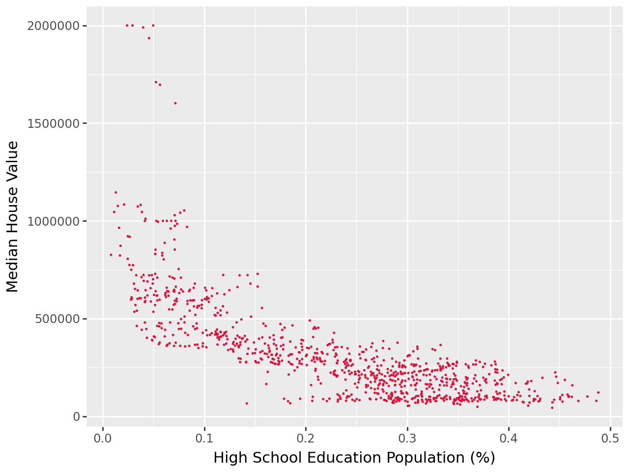
As part of exploratory data analysis, median house value was plotted alongside key features to determine possible correlations between our dependent variable and our predictors. In Figure 2a, median household income is shown to have a fairly strong positive linear correlation to median house value. In Figure 2b, white population % also shows a positive correlation, albeit much weaker and widely dispersed across the graph. In Figure 2c, high school education population % shows a negative correlation, with median house value decreasing as the proportion of the population with high school attainment increases.
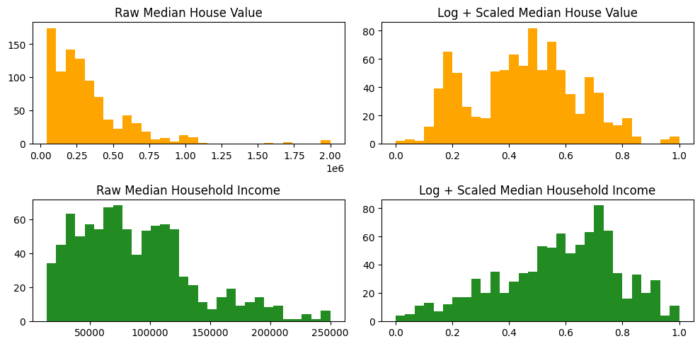
Further analysis of the data revealed median house value and median household income to both have right skew. To address this problem and normalize the data in preparation for models such as regression models, as part of preprocessing, median house value and median household income were both log-transformed. These variables were then scaled between 0 and 1 using MinMaxScaler to improve the performance of models such as neural networks, which are more sensitive to input ranges.
Race and educational attainment populations were turned into percentages of their respective census tract’s total population in order to provide a more accurate analysis of the composition of a tract, preventing data skew towards larger tracts with higher populations. These percentages are already between 0 and 1, meaning log-transformation and scaling were less necessary for these features.
In order to improve time-series data forecasting, two years of lagged house value data were added as features. These lag features allowed models like linear regression and neural networks to pick up on past trends over the two years prior. Only two years of lag data were added due to the limited size of the dataset.
The data was then split into X, the features including household income, racial composition, educational attainment demographics, and lag house value, and Y, the dependent variable of house value. In order to prevent perfect collinearity from the percentage-based features, percentage white population and percentage population with high school attainment were excluded, serving as the baseline for future models.
Lastly, the data was split into training and testing by years, with 2012-2020 being training and 2021-2022 being set aside as testing. Performing train-test split by years rather than random rows is necessary to prevent data leakage of future data, which would artificially improve the performance of the model and would be unrealistic as predictive models only have access to historical data.
Model Selection
The baseline model is an Ordinary Least Squares (OLS) regression model, trained on all features and evaluated on the test set. Similarly, a Least Absolute Shrinkage and Selection Operator (LASSO) model was constructed and trained to minimize mean squared error, using a penalty to automatically reduce features.
More complex models were constructed, including neural networks, Long Short-Term Memory (LSTM), and Extreme Gradient Boosting (XGBoost). Due to the iterative training and tuning processes of these models, 2020 data was set aside from training to be used as validation. The hyperparameters of the neural network were tuned both manually and with KerasTuner to determine the most effective and accurate model. These hyperparameters included number of layers, neurons, dropout rate, and learning rate. Early stopping was also used to avoid overfitting the model. However, due to the limitation of time-series forecasting, K-fold cross-validation could not be employed to increase robustness as taking random subsets of data could again cause leakage of future data into training. After running 100 random trials with the training and validation sets to determine the best set of hyperparameters, the final model was trained using all years 2012-2020. The best neural network was constructed using an input layer with 256 neurons, a hidden layer with 240 neurons and a dropout rate of 0.1, another hidden layer with 224 neurons and dropout rate of 0.1, ReLU activation function on all layers, a learning rate of 0.0003226, and compiled with Adam optimizer and MSE loss function.
Next, an LSTM model was constructed using past median house value as a time series feature in order to efficiently handle sequential data. A sliding window approach is taken where the previous few years are used to predict the next year of data, with the number of previous years used being determined by the sequence length. KerasTuner was again employed to tune the hyperparameters of the LSTM model, tuning the same hyperparameters used in the neural network as well as sequence length. The final model consists of a sequence length of 2, three LSTM layers with 48, 128, and 48 neurons respectively and a dropout rate of 0.1 on the first, a dense layer for output, a learning rate of 0.005009, and compiled with the Adam optimizer and MSE loss function.
Lastly, an XGBoost model was built, utilizing gradient-boosted decision trees to incrementally improve the model’s performance. Hyperparameters were tuned and optimized using Optuna. These hyperparameters included learning rate, max depth, subsamples, and regularization terms. The performance of each trial was assessed using the mean RMSE, calculated using walk-forward cross-validation to iterate over years in a chronological manner, preserving time-series order through a sliding window to better assess the performance of the model. Lastly, the model was evaluated on the test data and a feature importance plot was generated to highlight the most significant predictors.
Once all the models were built and evaluated against the test set, calculating MAE, RMSE, and R2 metrics, the best model was determined to be the neural network, with low MAE and RMSE values reflecting the least average error and fewer large errors. This model was then applied to predict house values for census tracts in the year 2023, with house value predictions iteratively fed back into itself to continue predictions of 2024 and 2025. Since the objective was to generate forecasts for 2023-2025, years where data for features were not yet available, feature values beyond 2022 were estimated using linear extrapolation from their historical trajectories. Household income, racial composition, and educational attainment percentages were each extended forward based on the best-fit linear regression line for the feature over the entire period. This approach preserves the temporal dynamics of these features, though it does make the assumption that there will not be abrupt changes to these socioeconomic and demographic characteristics. This introduces potential sources of bias, possibly misrepresenting true underlying values if future conditions deviate from past trends. Moreover, the linearity of this approach may underfit the complexity of real-world dynamics. However, given the relatively short forecast horizon, linear extrapolation was deemed sufficient to provide realistic and consistent feature estimates for model prediction. In addition to predictive modeling, this study maps and analyzes housing price, income distribution, and demographic trends across Mercer County. Mapping provides a clear representation of regional disparities and their correlations with other socioeconomic characteristics, helping to identify their consequences in the real estate market.
All code used in this study is available in the following GitHub repository: https://github.com/26kl0145/mercer-county-housing-analysis
Analytical Results
This section presents a geospatial analysis of housing price, income distribution, and racial composition throughout Mercer County, highlighting geographic disparities and trends through visualizations of the data. Mercer County is a highly diverse region with stark contrasts in home values and racial demographics across the area. The mapping data illustrates a clear spatial divide, with high median house values concentrated in the northern and eastern parts of the county in the Princeton area, while lower median house values and higher volatility are concentrated in the southwest in the Trenton area. These regions also loosely correspond to higher white and higher minority populations respectively. The following figures and tables reveal these observations and the results of an examination via predictive modeling.

The racial composition of Mercer County is an essential factor in understanding housing disparities. Figure 4 shows the census tracts within Mercer County and the percentage of their total population that identifies their race as Black or African American, American Indian or Alaska Native, Asian, Native Hawaiian or other Pacific Islander, two or more races, or other. A noticeable concentration of regions in the east and especially the southwest have a substantial portion of racial minority residents, while census tracts in the northwest and south mostly consist of white residents.

Educational attainment is another critical factor in determining the general wealth and prosperity of a region. Figure 5 displays the percentage of the total population in each census tract whose highest level of education is anywhere from no education received to high school. There is a higher concentration of this category among the western and eastern ends, with a notably high concentration in the southwest. Conversely, the northeastern region of Mercer County has a much lower concentration, indicating a greater portion of individuals who have received some form of higher education.

The relationship between median house values and geography becomes even clearer when examining Figure 6, which presents the median house values across Mercer County from 2012 to 2022. The northern and eastern areas, particularly around Princeton, display much higher median house values, with some census tracts having values exceeding $2 million. In contrast, the southwest, especially Trenton, shows significantly lower median house values, with many areas reporting values under $100,000.
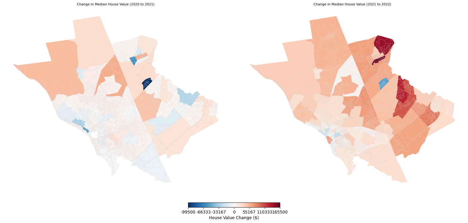
The year-to-year fluctuations in housing prices provide further context for understanding the housing market dynamics in Mercer County. Figure 7 shows the change in house value across census tracts between 2020 and 2021, and 2021 and 2022. Red areas indicate an increase in house value, while blue areas indicate a decrease in house value. The values are scaled between 0 and the largest change, with white indicating no change and the boldest sections representing the most significant increases or decreases.
Across both years, the northern and eastern edges tended to increase the most significantly, while most decreases in house value occurred in the southwest region. However, as shown in Figure 6, this section contains predominantly lower-value homes, so the actual change in terms of percentage may be different. The southwest also had much more variation in whether the house value increased or decreased, as many census tracts in the southwest experienced a decrease in median house value between 2021 and 2022 even while the vast majority of other census tracts were climbing in house value.
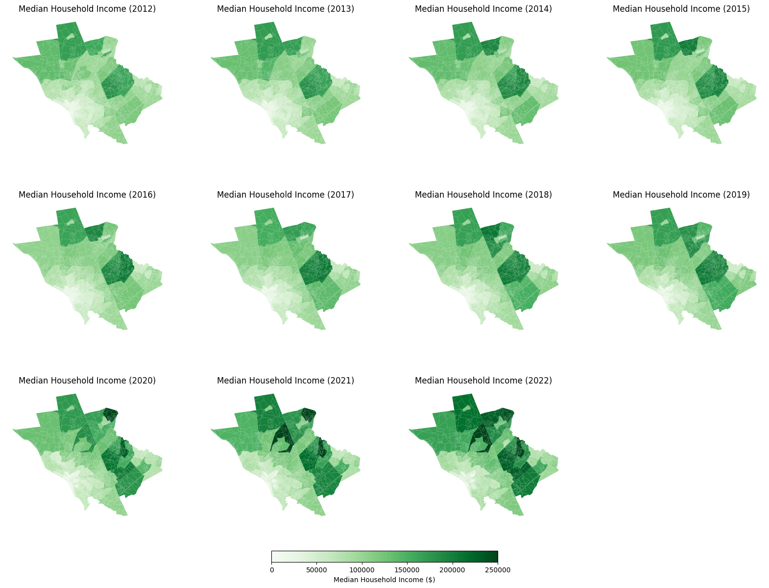
Figure 8 shows the median household income of each census tract within Mercer County from 2012 to 2022. Similar to Figure 6, the northern and eastern edges contain the tracts with the highest median incomes, while the southwest contains the tracts with the lowest median incomes. Unlike minority composition and under high school educational attainment, there seems to be much stronger changes in median household income across the years, especially on the northern and eastern edges, where median income has increased substantially since 2020.

The study uses a neural network model to predict median house values for the years 2023 to 2025 across Mercer County. Figure 9 displays the predicted median house value of each census tract within Mercer County for the years 2023, 2024, and 2025. Data from 2012-2020 were used as training and data from 2021-2022 were used for testing. The features used to train the model were median household income, racial composition percentages, educational attainment percentages, and two lag years of median house value to allow the model to capture short-term trends in house value.

Figure 10 displays the increases and decreases in predicted median house values between years as a percentage change from the year prior. The percentages plotted are all between -15% to 15%, with red areas indicating increases in house value and blue areas indicating decreases in house values. Areas exceeding this boundary have been plotted in separate colors in order to increase interpretability of the colorbar. Tracts colored in gold were predicted to have house price increase by over 15%, while tracts colored in purple were predicted to have house price decrease by over 15%. Most tracts affected by this change are located in the southwest region, with one tract in particular predicting a 40% decrease in house value.
From 2022 to 2023, the model mostly estimated substantial decreases in house value, with only a few scattered tracts estimating moderate increases. From 2023 to 2024, the model was more varied in its estimates, predicting increases and decreases across Mercer County. In general, tracts that saw increases in house value between 2022-2023 were predicted to have more pronounced increases between 2023-2024, while tracts that saw decreases in house value between 2023-2024 were now predicted to either increase in house value or have less severe decreases. This trend continues from 2024-2025, with more census tracts having increases in median house value, with some of the census tracts that experienced the highest decreases now experiencing the largest growth in house value. Of note throughout all predictions is the southwest region, which contained both large increases and large decreases in house value throughout all tracts.
Model Evaluation
To evaluate the prediction model and look for the best one to predict the housing market, several types of models were created, training and validating on data over 2012-2020 and testing on data over 2021-2022.
| Model | MAE | RMSE | R2 |
|---|---|---|---|
| OLS Regression | 24642.57 | 36289.24 | 0.986 |
The baseline model is a linear regression model, trained using all features to predict house value. For this model median house value and median household income were log-transformed, as a normal distribution is necessary for linear regression to hold true. However, they were not scaled using MinMaxScaler in order to keep regression results interpretable. Metrics were inverse log-transformed after predictions.
As indicated by the R2 value of 0.986, the model performs very well, explaining 98.6% of the variance in house value. However, this fit is largely driven by lag-1 house value, the house value data from the year prior, which had a coefficient of 0.9711 and a p-value of 1.99e-54, indicating extreme significance. This coefficient indicates that a 1% increase in last year’s house value predicts nearly a 1% increase this year. This persistent relationship is to be expected, as housing markets do not fluctuate wildly from year-to-year. Conversely, lag-2 house value, the house value data from two years prior, has a coefficient of -0.0583 and a p-value of 0.295, indicating poor significance. This is likely because after accounting for the first lag, the second lag adds little to prediction.
Household income is also a significant positive predictor, with a coefficient of 0.0366 and a p-value of 0.031. This coefficient indicates that increasing median household income by 10% is associated with an increase of approximately 0.37% in house value.
For the other two feature categories, race population and educational attainment, baselines were taken to avoid perfect collinearity, those being white population and high school educational attainment. As such, any coefficients within these categories are interpreted relative to high school graduates. For educational attainment, associate degree, professional degree, and doctorate degree were all positive and significant, with coefficients of 0.4712, 0.6242, and 0.2882 respectively and p-values around 0.01. Since the dependent variable is log-transformed house value and population shares are between 0 and 1, the effect on house value can be calculated as
where $latex \beta$ is the coefficient and $latex \Delta X$ is the change in the share of the population (0-1 scale) from the baseline to the feature. For example, if 10 percentage points of the population moved from high school graduates to associate degree holders ($latex \Delta X = 0.1$), the model predicts house values would increase by about 4.8%, holding other factors constant. Although no other educational attainment levels were significant at the level α = 0.05, kindergarten educational attainment had a p-value of 0.063 and is of note due to its large negative coefficient of -7.6215. A 10 percentage point change in population from high school graduates to kindergarten educated is predicted to change house values by -53.3%, holding other factors constant. Although most educational levels were not statistically significant, according to the coefficients, the general trend in educational attainment suggested that relative to areas with more high school graduates, the model predicted areas with more degree-holders to have increased house values, while areas with more residents with less than high school education were associated with decreased house values.
For race, all categories were insignificant at the level α = 0.05, suggesting that racial composition does not show a significant independent association once other factors are controlled for. However, it is notable that all racial demographics except for Black population had negative coefficients, indicating that increasing the share of most minority populations relative to the white population is associated with decreased house values.
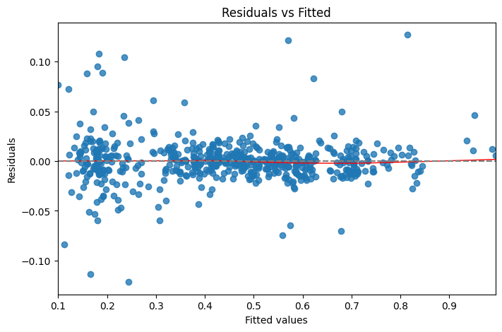
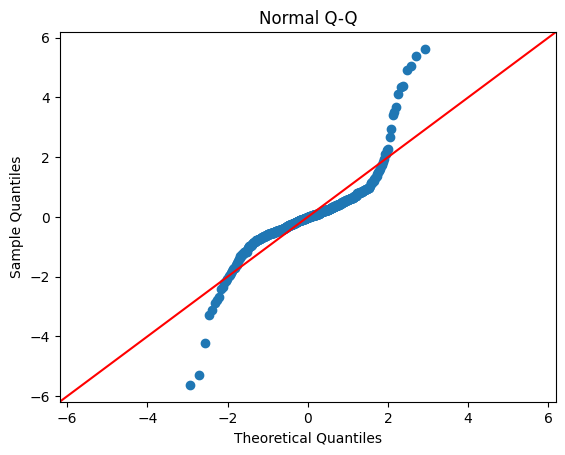
To test the assumptions necessary for linear regression, residual diagnostic plots were created to analyze the model. As shown in Figure 11a, the model meets both linearity and homoscedasticity due to the random spread of points around the horizontal line at zero. This indicates that the residuals are randomly distributed. However, Figure 11b reveals significant departures from normality, with the shape indicating heavy tails in the residual distribution.
| Model | MAE | RMSE | R2 |
|---|---|---|---|
| LASSO | 23566.60 | 35495.35 | 0.986 |
After the linear model, a LASSO model was constructed using all features and the lambda value that minimized MSE. This model performed quite strongly as well, with similar metrics to the OLS regression model. The features selected by the model at the minimum lambda value were median household income, other racial composition percentage, 9th-10th grade educational attainment, some college education, bachelor’s, master’s, professional, or doctorate degree, and the first lag year of house value. Median household income, the lag year of median house value, and all education from a bachelor’s degree and above had positive coefficients. All other selected features had negative coefficients, notably including other racial composition percentage, which refers to individuals whose race doesn’t identify as white, Black, American Indian, Alaska native, Asian, native Hawaiian and other Pacific Islander, or two or more races.
| Model | MAE (mean ± std) | RMSE (mean ± std) | R2 (mean ± std) |
|---|---|---|---|
| Neural Network | 31052.51 ± 6933.07 | 46356.51 ± 9956.08 | 0.975 ± 0.011 |
The next model created was a neural network, trained using all features. Median household income and median house value were both log-transformed and scaled using MinMaxScaler in order to increase robustness by ensuring the larger value ranges of these features do not dominate the learning process. After determining the optimal hyperparameters for the model through KerasTuner, the model was trained on data from 2012-2020 and tested 30 times on the testing set from 2021-2022 to determine the mean evaluation metrics of the model, with standard deviation included as well.
The performance of the model is weaker than the OLS regression and LASSO, with higher MAE and RMSE and a lower R2 value. The model introduces inherent randomness due to the nature of neural networks and the inclusion of dropout layers, randomly deactivating neurons in order to reduce overfitting. However, the standard deviations are still reasonable, suggesting model training is stable.
| Model | MAE (mean ± std) | RMSE (mean ± std) | R2 (mean ± std) |
|---|---|---|---|
| LSTM | 45415.17 ± 3103.16 | 70038.51 ± 7021.05 | 0.946 ± 0.011 |
Following the neural network, an LSTM model was built in order to try and capture trends across the time-series data through its unique capabilities in processing sequential data. A similar process to the neural network was utilized for training the LSTM, again preprocessing features using log-transformation and MinMaxScaler and using KerasTuner to identify optimal hyperparameters, including sequence length.
The model performed noticeably worse than the neural network, with both higher error and lower R² Although LSTMs are designed to handle sequential data by storing data over time steps, they are more so built to capture long-term dependencies in data, which this dataset does not contain in its 11 years of data spanning 2012-2022. The neural network, on the other hand, does not rely on long-term trends, so training the model using just two lag years of data likely allowed the neural network to sufficiently capture relationships in house value. This lack of data likely also explains why the LSTM model obtained through tuning had a sequence length of 2, indicating that focusing more on recent years had much greater success in predictions than trying to find long-term dependencies.
| Model | MAE (mean ± std) | RMSE (mean ± std) | R2 (mean ± std) |
|---|---|---|---|
| XGBoost | 33746.09 | 79126.60 | 0.931 |
The last model constructed was an XGBoost model due to its efficient and effective training process as well as its interpretability, implementing gradient boosted decision trees that perform well in regression tasks. After preprocessing, Optuna and walk-forward cross-validation were utilized to train the model and tune hyperparameters, ensuring optimization without leaking future information into the model and evaluating the model’s predictions on unseen data by preserving the temporal ordering of the data.
For the neural network models, results were averaged across multiple trials since weight initialization and training order introduce inherent randomness, which can cause variability in performance. As such, both mean performance and standard deviation are reported. In contrast, the XGBoost models are deterministic given fixed data and hyperparameters. Repeated runs under identical conditions yield identical outcomes (standard deviation = 0). As such, single metrics for MAE, RMSE, and R² are reported for XGBoost.
The MAE of the XGBoost model is comparable to the neural network, but its RMSE is significantly higher despite being optimized to reduce RMSE. The R² value is also weaker than that of both the neural network and the LSTM. This is likely due to the nature of decision trees, which capture piecewise splits rather than continuous relationships. As illustrated in Figure 2, many features have at least a somewhat linear relationship with house value, meaning the steps created by the model may not effectively approximate these trends. XGBoost is also less flexible in capturing interactions between features, especially with the lag features of house value, as it treats each feature separately and cannot capture these temporal patterns effectively.
From the feature importance plot of the model, the two lag features of house value were by far the most important in predicting house value, which is to be expected. Following these features are household income, educational attainment at bachelor’s or above, 10th grade, 6th grade, associate’s degree attainment, and then Asian population. Like the regression models, the most important features continue to be household income and attainment of higher education. Unlike those models, however, is the inclusion of Asian population percentage as an important feature. Unfortunately, XGBoost does not provide information on whether this was positively or negatively correlated with house value, so the effect of an increase in the share of population of Asians cannot be determined.
| Model | MAE | RMSE | R2 | Additional Notes |
|---|---|---|---|---|
| OLS Regression | 24642.57 | 36289.24 | 0.986 | |
| LASSO | 23566.60 | 35495.35 | 0.986 | |
| Neural Network | 31052.51 ± 6933.07 | 46356.51 ± 9956.08 | 0.975 ± 0.011 | Mean ± Std (30 trials) |
| LSTM | 45415.17 ± 3103.16 | 70038.51 ± 7021.05 | 0.946 ± 0.011 | Mean ± Std (30 trials) |
| XGBoost | 33746.09 | 79126.60 | 0.931 |
Although the linear model and LASSO demonstrate better performance on the standard evaluation metrics for the test set, the neural network is still retained as the final model for forecasting. The primary reason is its ability to capture non-linear relationships and complex interactions among features that may not be evident in historical data but are likely to influence future trends, especially with larger datasets spanning greater periods of time. Subtle patterns in growth rates, socioeconomic factors, and demographic shifts may produce non-linear effects on house values. As such, a neural network, even if it underperforms on short-term test metrics, is more flexible to unseen future scenarios and provides a more robust and adaptable prediction framework. Moreover, the linear model is rigid and assumes strictly linear relationships, while the neural network allows for the incorporation of other features that may not have these relationships.
Discussion
The findings from the previous analysis clearly highlight significant economic and housing disparities across Mercer County, particularly between the affluent northern regions and the economically challenged southwest. The following discussion will explore these findings in greater depth.
As evident in the analytical results, the Trenton area in the southwest of Mercer County was consistently the least wealthy region in the county, with the lowest median house value and median household income. Significantly, the bottom three income quintiles were concentrated almost entirely within this southwestern portion of the county. The change in median house value across years also varied most highly in the southwest region, as exemplified from 2021 to 2022 in Figure 7 (change in house value between years, 2020-2022). The map of the predicted house values (Figure 9) maintained this trend, with the highest value houses still notably prevalent among the north and northeastern edges of Mercer County while the census tracts with the lowest median house values were still in the southwest. The southwest region is further characterized by having the highest concentration of minority populations (Figure 4), suggesting a possible correlation between race demographics and the affluence of neighborhoods in Mercer County. The high variance in house value changes (Figure 7) in the Trenton area compared to the rest of Mercer County also suggests that less wealthy communities experience greater economic instability and grow less consistently with broader house value appreciation trends. The northernmost region of Mercer County is also a mostly minority population, while simultaneously having by far the highest median house values, further suggesting the correlation between affluence and race demographics. However, as revealed along the northeastern edge of Mercer County, which was in the top quintile for median house value and also one of the regions with larger minority populations (Figure 4), the trend observed in the Trenton area doesn’t necessarily indicate a broader trend across Mercer County or other regions.
The predicted values for median house value varied quite significantly between years (Figure 10). In general, housing prices were largely predicted to decrease between 2022 and 2023, with the exception of a few scattered census tracts that experienced substantial increases. Between 2023 and 2024, decreases in house value were less severe while more tracts saw increases instead, suggesting a forecasted upturn in house value, especially around central Mercer County. This trend continues from 2024-2025, with fewer census tracts predicting decreases in house value, most of which are located around the edges and southern region of Mercer County. These trends suggest that the model saw significant signs of increasing house value in central Mercer County. However, outside of this region, the model predicted fairly broad increases in house value, indicating that the model did not see particular guiding trends upward or downward elsewhere in Mercer County, further indicating limited correlation between property growth and demographic characteristics in regions such as Trenton.
Among the predictive models, the OLS regression and LASSO models performed the best, with the latter performing slightly better. This is indicative of roughly linear relationships between features such as median household income and the target variable, median house value. This is especially true of the lagged house values, which often increase relatively smoothly compared to features like racial composition. In such cases, more complex models may not provide additional predictive power, while a linear regression model is able to capture these relationships well. The limited sample size, both in years and total census tracts, may also contribute to this performance, as models like neural nets are prone to overfitting on the training data while linear regression models remain more stable.
However, as stated previously, the neural network may still be valuable for long-term forecasting. Unlike linear regression, the neural network can capture nonlinear relationships among socioeconomic factors that may become more pronounced as census data expands and income, demographic, and educational distributions shift. This flexibility could allow the neural network to better adapt to long-term structural changes in the data, even if its short-term performance is not as strong as the linear models.
Analysis of Figure 4 (racial minority population, 2012-2022), Figure 6 (median house value, 2012-2022), and Figure 10 (% change in predicted median house value) suggest that regions with high populations of racial minorities experience slower property growth and higher instability and volatility in their economic security, especially within the Trenton area, which possesses among the lowest population of white residents and the lowest median house values in Mercer County. Despite these qualities, many other regions across Mercer County did not see similar trends, and analyses of Figure 7 (change in median house value, 2020-2022) and predictions of future house value showed limited evidence of the hypothesized stagnant growth in Trenton and rapid growth only within the Princeton area.
These may be attributable to ongoing development projects in Mercer County, such as Trenton250, a long-term plan for stimulating innovation and growth across Trenton. Goals of the project include promoting downtown economic development, redeveloping industry, and constructing more affordable and convenient transportation options. By improving the locational attributes and amenities of Trenton, housing in Trenton would become much more valuable, increasing the demand for housing and subsequently its prices. This gentrification of urban Trenton may stimulate the economy of the region and boost housing prices, though such development plans also run the possibility of displacing the large Black or Hispanic communities that currently make up the vast majority of Trenton residents.
Conclusion
This study provides important insights into housing inequality in Mercer County, New Jersey, by examining trends in housing prices, income distribution, and racial composition over the past decade, all through the lens of a deep learning approach. The results highlight clear economic disparities between the northern and southern regions of the county. In particular, growth remains higher and steadier around the Princeton area in the north, while the Trenton area in the southwest by contrast experiences lower property values and greater price fluctuations and instability. These differences align with the racial makeup of the regions, with Trenton predominantly consisting of minority communities, suggesting a correlation between house value and racial demographics. However, this apparent correlation may be spurious. Racial demographics typically experience little change over time, so a decline in house value in an area with a large minority population may create a false impression of a relationship between the two, when in reality, they may be driven by other factors, such as changes in infrastructure. Furthermore, as indicated by regression results and predictive modeling, there is not sufficient evidence to reject the null hypothesis that house value and racial demographics are not correlated to one another, holding all other variables constant. Instead, features like household income and educational attainment provide a much more direct correlation to house value. As such, historical and structural factors may still be correlated with the housing market in certain sections of Mercer County, reinforcing long-standing patterns of residential segregation. The trends of economic inequality and instability are unlikely to change without significant shifts in housing policy, infrastructure development, and economic opportunities.
However, this study does include several limitations. A primary limitation lies in the variables studied. While median household income and educational attainment certainly hold relevance to median house value, there are bound to be many other characteristics of Mercer County that shape its economic trends. Furthermore, factors such as informal housing dynamics and local policy changes may not be fully captured by publicly available census data. The reliance on census data could also introduce potential biases or miss emerging trends in the housing market. In addition, although the neural network model proves to be a powerful tool for identifying complex relationships between features, they are prone to overfitting and may fail to adequately capture short-term fluctuations driven by sudden economic or policy shifts. To address these challenges in future research, incorporating real-time data sources or experimenting with alternative machine-learning models could enhance accuracy.
There are several promising approaches for expanding on these findings. One important direction is to integrate qualitative research, such as interviews with local residents or analysis of policies and their impacts. This approach would offer a more nuanced understanding of the experiences of these communities with housing markets and inequality. A comparative study of other cities facing similar socioeconomic challenges could also offer valuable insights into how these trends play out in different urban settings. Additionally, future studies could incorporate other dynamics within the real estate market, including affordable housing projects and migration patterns, in order to provide a fuller picture of the many factors influencing housing trends. Incorporation of more diverse socioeconomic features could further refine predictive models and improve their practical applications predicting real-world housing market scenarios. Related features could include employment, occupation type, age distribution, household size, commute time to work, and especially features directly related to housing, such as housing vacancy rates and housing cost burden. Future research could also incorporate data and indices utilized in the Justice40 initiative, which include but are not limited to factors like social vulnerability and health inequality. Discussion on geospatial data on redlining borders could provide additional insights into past segregation practices.
To further enhance predictive models, several strategies can be tested. In this study, MinMaxScaler was utilized to scale median house value and median household income in order to ensure effective analysis of features by gradient-based models like neural networks and LSTMs. However, MinMaxScaler is more sensitive to outliers, possibly making learning harder by excessively shrinking other values if outliers are present. Median house value especially includes several such outliers that may have impacted model performance. Other feature scaling techniques, such as RobustScaler or StandardScaler, may increase predictive accuracy of models by preventing such outliers from drastically impacting the scale. RobustScaler in particular may also enhance the OLS regression and LASSO models by further normalizing distributions, albeit at the cost of interpretability of coefficients. Furthermore, walk-forward CV, as used in training the XGBoost model, could also be implemented into the other models to simulate real forecasting conditions, evaluating the model over time and providing a more generalized model. Walk-forward CV would thus prevent overfitting to the training data, likely enhancing predictive accuracy. Using hybrid tree-based models or multi-level neural networks, such as those used by Sibindi and colleagues and Wijaya14 16, may reveal much stronger correlations and trends between features, especially in the long-run. Finally, while this study addressed ACS limitations through tract-splitting adjustments and interpolation, future work could explore alternative approaches to handling ACS limitations. These include analyzing and aggregating to larger geographic regions in order to reduce sampling error, using harmonized boundary datasets to maintain consistent geographies, or comparing multiple imputation methods to assess robustness. A sensitivity analysis for forecasting future house values using linear interpolation vs. forward fill for features could be performed in order to determine if using linear interpolation has significant impacts on model predictions in the short or long run.
In summary, this paper makes several contributions to the literature on housing price prediction. First, this research highlights the significant potential of deep learning models, specifically neural networks, in forecasting housing price trends. While OLS regression and LASSO achieved better evaluation metrics than the neural network, the neural network provides strong predictive capacity and a flexible framework for future time-series forecasting. Second, the comparative evaluation between OLS regression, LASSO, neural networks, LSTM, and XGBoost highlights the importance of model selection in housing market research and shows that tree-based and sequence-based models may underperform when applied to short-term structured socioeconomic data. Third, by combining predictive models with geospatial visualization, this study provides an integrated approach for exploring spatial distribution of housing value trends and their correlations with income, education, and racial composition. These contributions underscore both the promise and limitations of different machine-learning methods while offering a framework for analyzing localized housing disparities. By shedding light on these dynamics, the study offers important insights that can inform future research and policy-making efforts focused on addressing housing inequality throughout Mercer County. Ultimately, these findings contribute to the broader goal of fostering greater inclusivity and equality in housing markets.
- U.S. Department of Housing and Urban Development, Office of Policy Development and Research. (2021). Comprehensive housing market analysis for Trenton-Princeton, New Jersey. https://www.huduser.gov/portal/publications/pdf/TrentonPrincetonNJ-CHMA-21.pdf [↩] [↩]
- Özmen, M. U., Kalafatcılar, M. K., & Yılmaz, E. (2019). The impact of income distribution on house prices. Central Bank Review, 19(2), 45-58. https://doi.org/10.1016/j.cbrev.2019.05.001 [↩]
- Gallin, J. (2006). The long-run relationship between house prices and income: Evidence from local housing markets. Real Estate Economics, 34(3), 417-438. https://doi.org/10.1111/j.1540-6229.2006.00172.x [↩]
- Chen, M.-C., Tsai, I.-C., & Chang, C.-O. (2007). House prices and household income: Do they move apart? Evidence from Taiwan. Habitat International, 31(2), 243-256. https://doi.org/10.1016/j.habitatint.2007.02.005 [↩]
- Reichert, A. (1990). The impact of interest rates, income, and employment upon regional housing prices. The Journal of Real Estate Finance and Economics, 3(4). https://doi.org/10.1007/bf00178859 [↩]
- De Bruyne, K., & Van Hove, J. (2013). Explaining the spatial variation in housing prices: An economic geography approach. Applied Economics, 45(13), 1673-1689. https://doi.org/10.1080/00036846.2011.636021 [↩]
- Case, K. E., & Mayer, C. J. (1996). Housing price dynamics within a metropolitan area. Regional Science and Urban Economics, 26(3-4), 387-407. https://doi.org/10.1016/0166-0462(95)02121-3 [↩]
- Nolan, B., Roser, M., & Thewissen, S. (2016). GDP per capita versus median household income: What gives rise to divergence over time? LIS Working Paper Series, No. 672. Luxembourg Income Study (LIS), Luxembourg. https://hdl.handle.net/10419/169232 [↩]
- Steegmans, J., & Hassink, W. (2017). Financial position and house price determination: An empirical study of income and wealth effects. Journal of Housing Economics, 36, 8-24. https://doi.org/10.1016/j.jhe.2017.02.004 [↩]
- Elwell, C. K. (2014). The distribution of household income and the middle class. Congressional Research Service (CRS) Reports and Issue Briefs. https://hdl.handle.net/1813/79194 [↩]
- Tsatsaronis, K., & Zhu, H. (2004). What drives housing price dynamics: Cross-country evidence. BIS Quarterly Review, March 2004. Available at SSRN: https://ssrn.com/abstract=1968425 [↩]
- Hanna, B. G. (2007). House values, incomes, and industrial pollution. Journal of Environmental Economics and Management, 54(1), 100-112. https://doi.org/10.1016/j.jeem.2006.11.003 [↩]
- Voith, R. (1991). Transportation, sorting and house values. Real Estate Economics, 19(2), 117-137. https://doi.org/10.1111/1540-6229.00545 [↩]
- Sibindi, R., Mwangi, R. W., & Waititu, A. G. (2022). A boosting ensemble learning based hybrid light gradient boosting machine and extreme gradient boosting model for predicting house prices. Engineering Reports, 5(4). https://doi.org/10.1002/eng2.12599 [↩]
- Adetunji, A. B., Akande, O. N., Ajala, F. A., Oyewo, O., Akande, Y. F., & Oluwadara, G. (2022). House price prediction using random forest machine learning technique. Procedia Computer Science, 199, 806-813. https://doi.org/10.1016/j.procs.2022.01.100 [↩]
- Wijaya, R. (2023). Multi level dense layer neural network model for housing price prediction. arXiv. https://doi.org/10.48550/arXiv.2310.08133 [↩]
- Zhu, E., & Sobolevsky, S. (2018). House price modeling with digital census. arXiv. https://doi.org/10.48550/arXiv.1809.03834 [↩]
- Zhao, Y., Ravi, R., Shi, S., Wang, Z., Lam, E. Y., & Zhao, J. (2022). PATE: Property, amenities, traffic and emotions coming together for real estate price prediction. arXiv. https://doi.org/10.48550/arXiv.2209.05471 [↩]
- Beginning of an industrial giant. (n.d.). Mercer County, NJ. https://www.mercercounty.org/community/history/beginning-of-an-industrial-giant [↩]
- Luckie, P. (2024). The social cost of deindustrialization: Postwar Trenton, New Jersey. Teaching Social Studies, 24(1). https://teachingsocialstudies.org/2024/02/21/the-social-cost-of-deindustrialization-postwar-trenton-new-jersey/ [↩]
- Nelson, R. K., & Winling, L. (2023). Mapping inequality. Digital Scholarship Lab. https://dsl.richmond.edu/panorama/redlining [↩]


