Detecting Fraud Insurance Claims Using Machine Learning

Abstract

Car insurance fraud poses a significant financial threat to insurance companies and economies, with an estimated 20–30% of global claims suspected to be fraudulent. This study investigates the detection of fraudulent car insurance claims using machine learning models while addressing the challenge of class imbalance in real-world datasets. Using a dataset of 15,419 claims (923 fraud, 14,496 non-fraud), extensive preprocessing and exploratory data analysis were conducted to uncover patterns and relationships among features. Models including Logistic Regression, K-Nearest Neighbors, XGBoost, and Random Forest were applied, with performance evaluated using precision, recall, and F1-score metrics. Various sampling strategies —class weighting, undersampling, and SMOTE-based oversampling—were employed to mitigate data imbalance, with Random Forest trained on undersampled data yielding the best performance (F1-score = 0.80 for fraud detection). Feature importance analysis using SHAP revealed “Fault,” “Policy Type,” and “Month Claimed” as critical predictors of fraud. The study also highlights the limitations of prior research, which often fails to report specific class-wise metrics in imbalanced datasets. Overall, the results demonstrate that tree-based ensemble methods, especially with effective sampling, significantly improve fraud detection performance. The findings offer valuable insights for developing robust, interpretable, and scalable fraud detection systems and lay the groundwork for future enhancements through data balancing, cost-sensitive learning, and integration of unstructured claim data.

Introduction

Car insurance fraud happens when fraudsters deliberately deceive an insurance company to gain financial benefit through fake accidents, exaggerated damages and staged collisions. These lead to insurance companies giving the fraudsters the benefits causing financial losses and eroding trust in the company. Due to the evolving nature of fraudulent schemes, it is hard to distinguish between legitimate and fraudulent claims. An estimated 20% to 30% of global insurance claims are suspected to be fraudulent Ding et al. (2024)¹. This equates to billions of dollars in losses for the insurance industry destabilizing the economy of the nation. As the insurance companies need to pay compensation fees to clients to save their reputation and trust, it becomes necessary for companies to detect these frauds. Hence, car insurance fraud detection is crucial as it protects insurers, policyholders and the economy from facing losses worth billions of dollars. Auto insurance fraud detection utilizes various techniques, including data analytics, machine learning, and artificial intelligence (AI), to identify and prevent fraudulent insurance claims. These methods analyze the claim data patterns, policyholder behavior, and other factors to predict and flag suspicious and fraudulent activities, aiding insurance companies in efficiently managing fraud and saving them from losses.

Automobile insurance fraud represents a pivotal percentage of property insurance companies’ costs and affects the companies’ pricing strategies and social economic benefits in the long term. As the fraud types and patterns are evolving day by day, it is important to have a clear understanding of how different technologies are used for fraud detection. There are different aspects to solve while detecting frauds in car insurance claims. Aslam et al. (2022)² conducted a study which presents a comprehensive framework for detecting auto insurance fraud using machine learning (ML) models. Their objective was to to build an effective and accurate fraud detection model for the auto insurance industry using AI and ML techniques. They used a publicly available dataset of US auto insurance claims with 33 features. They applied boruta algorithm to identify 9 significant features (e.g. Fault, Base Policy, Age of Policyholder). ML models used in the study were Logistic Regression (LR), Support Vector Machine (SVM) and Naïve Bayes (NB). SVM had the highest accuracy (94%) and specificity (99.77%). Logistic Regression performed best on recall (42.25%), F1-score (29.26%), and sensitivity (42.25%). Naïve Bayes had the highest precision (23.07%). Their limitation is they focused only on US-based auto insurance data. Finally they suggested expanding to other regions and applying advanced techniques like: Deep learning, Ensemble models and PCA and genetic algorithms for better feature engineering.

Wang et al. (2018)³ conducted a study which proposes an innovative approach for detecting fraudulent automobile insurance claims by combining Latent Dirichlet Allocation (LDA) with Deep Neural Networks (DNNs). Their objective was to enhance the accuracy of insurance fraud detection by integrating text mining (using LDA) with deep learning, especially focusing on unstructured text data in insurance claims. They incorporated textual descriptions which traditionally ignore text description in claims, and used LDA to extract topics (e.g., accident details, responsibility, damage). These topics are used as additional features for the detection model. They used a deep neural network (DNN) that uses both structured data (numeric/categorical) and LDA-generated topics. The DNN learns complex patterns for better fraud detection. For the dataset, they used real-world data with 37,082 insurance claims (only 415 were fraudulent). DNN with LDA outperformed both RF and SVM, showing accuracy of 91.4%, precision of 91.7% and F1-score of 91.3%. On comparing DNN without LDA, the accuracy improved by 6.8%, F1 by 7.2%. Their study confirms that combining LDA topic modeling (for textual claim descriptions) with deep learning provides a more powerful tool for detecting automobile insurance fraud than traditional methods.

Both studies did not provide separate performance metrics for the fraud and non-fraud classes. In such a highly imbalanced dataset, fraudulent classes are underrepresented and reporting only aggregate metrics can be highly misleading. Their precision, recall and f1 scores appear very impressive but are highly influenced by the dominant non-fraud class. Their models’ high overall accuracy may primarily reflect the model’s performance on the majority class (non-fraud). To make well-informed decisions in practical applications, especially in high-stakes areas like insurance fraud, it’s essential to evaluate and report performance metrics separately for each class, particularly focusing on recall and precision for the minority (fraudulent) class.

Chawla et al. (2002)⁴ introduced the Synthetic Minority Oversampling Technique (SMOTE), which generates synthetic samples by interpolating between minority class instances instead of simply duplicating them. This approach proved effective in addressing skewed class distributions across a wide range of domains, including fraud detection. Building on this, Chawla et al. (2003)⁵ proposed SMOTEBoost, which integrates SMOTE into the boosting framework to enhance the predictive performance of minority class detection. Their work demonstrates that resampling strategies combined with ensemble learning can significantly improve detection rates of fraudulent instances, complementing the SMOTE-based experiments presented in this study.

Subsequent research has emphasized that integrating oversampling methods with ensemble learners leads to more robust fraud detection models. Batista et al. (2004)⁶ and later works showed that combinations such as SMOTE with bagging or boosting provide superior recall rates for minority classes while maintaining stability in overall accuracy. Such findings align with the outcomes observed in our study, where Random Forest and XGBoost achieved high performance when applied to resampled data. This supports the conclusion that ensembles paired with data-balancing methods form an effective strategy for handling the imbalance in insurance claim datasets.

In contrast to data-level solutions, cost-sensitive learning directly incorporates class imbalance considerations into the training process by assigning higher penalties to misclassified fraudulent claims. Araf et al. (2024)⁷ highlighted that cost-sensitive methods often outperform naive oversampling by avoiding the introduction of synthetic noise, especially in cases where false negatives are particularly costly. For insurance fraud detection, where undetected fraudulent claims result in significant financial losses, this approach represents a viable alternative to resampling. Although not implemented in this study, cost-sensitive algorithms are an important direction for future research.

Another promising direction involves algorithm-level adjustments through modified loss functions. Lin et al. (2017)⁸ introduced focal loss to focus model training on hard-to-classify examples, thereby improving performance on rare events without altering the data distribution. More recent work has extended this idea with multi-stage focal loss adaptations tailored for highly imbalanced financial datasets. These methods provide a model-centric solution to imbalance, making them an attractive alternative or complement to oversampling and cost-sensitive approaches for insurance fraud detection.

Recent review articles emphasize that the most effective fraud detection frameworks combine multiple strategies, including data augmentation, cost-sensitive learning, and ensemble modeling. Araf et al. (2024)⁷ and related surveys highlight that hybrid methods not only balance predictive accuracy and recall but also improve generalizability across datasets. Such findings validate the methodology applied in this paper, where SMOTE, ensemble models, and interpretability techniques such as SHAP were jointly leveraged. This supports the broader consensus that a multi-pronged approach is essential for effectively tackling the challenges of fraud detection in imbalanced domains.

Building upon this, recent studies from 2023 to 2025 have introduced advanced frameworks that further enhance the effectiveness of fraud detection systems through hybrid and interpretable learning approaches. Nabrawi (2023)⁹ demonstrated that applying both machine learning and deep learning methods, combined with class rebalancing strategies such as SMOTE, significantly improves fraud identification accuracy in healthcare insurance claims. du Preez (2024)¹⁰ conducted a comprehensive review of fraud detection models and emphasized that ensemble learning and data augmentation are central to addressing class imbalance and generalizability challenges in imbalanced datasets.

Similarly, Curtis et al. (2025)¹¹ reviewed distinct machine learning classifiers used for healthcare fraud detection, highlighting that hybrid and cost-sensitive models outperform traditional single-algorithm systems. Matloob et al. (2025)¹² advanced this direction by developing adaptive deep learning architectures that dynamically adjust to emerging fraud patterns, demonstrating improved model adaptability across domains.

Furthermore, Gupta et al. (2024)¹³ proposed integrating blockchain technology with machine learning for insurance claim management, showing that secure, traceable data pipelines can enhance the reliability and interpretability of automated fraud detection frameworks. Collectively, these recent works reinforce the shift toward hybrid, explainable, and data-centric approaches—consistent with the multi-pronged methodology applied in this study.

The objective of this study is to analyse and identify which factors are significant to determine whether a car insurance claim is fraudulent or not. We also aim to develop an effective simple, yet predictive model to identify the fraud car insurance claims from not fraud with reasonable degree of accuracy. Lastly, we aim to use different sampling techniques to help understand which techniques work best for imbalance datasets. This will help companies in predicting whether a claim is fraudulent or not and save themselves from huge financial losses. This paper will break down all the steps so that future aspirants get to know about AI fraud detection in detail and how it works in real life scenarios.

Dataset

The dataset consists of 15,419 car insurance claims Kapoor (2025)¹⁴. Out of the 15,419 claims, 923 are fraud and 14,496 are non fraud indicating a high imbalance. The dataset contains 32 columns each one has its own purpose related to fraud found. The columns are categorized as time period, vehicle, driver, accident, policy and claims. Time period includes month, week of the month, day of the week, day of the week claimed, month claimed, week of month claimed. Vehicle includes vehicle category, vehicle price, make of vehicle, number of cars and age of vehicle. Policy and claim includes policy type, policy number, age of policyholder, base policy, fault, rep number, agent type, address change claim, past number of claims, days of policy accident, days of policy claim and age of policyholder. Driver includes driver rating, age, sex, deductible, marital status and fraud found. Accident includes area of accident, year, number of supplements, police report filed and witness present.

Exploratory Data Analysis

In this section, we explore different variables of the dataset and study their relationship to understand their significance in detecting fraud claims. The aim is to understand patterns, trends and relationships between variables. Understanding the patterns can help us to build an effective model.

Figure 1 illustrates count distribution of fraud and non fraud insurance claims. It appears that out of the 15419 claims, 923 are fraud and 14496 are non fraud indicating a significant data imbalance.

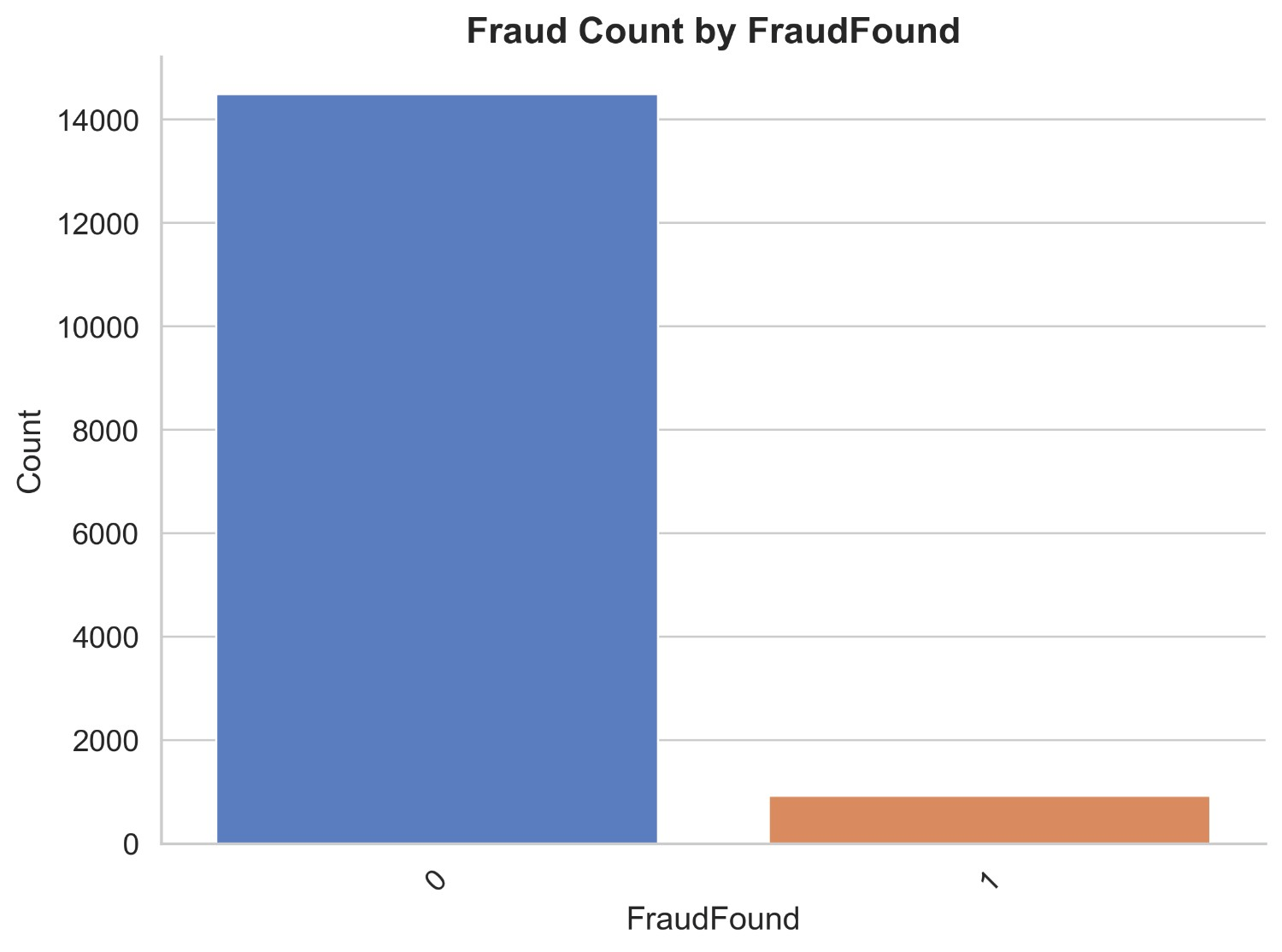
Figure 2 illustrates count distribution of fraud found or not based on the accident area. It appears that in urban areas there are 2 non-fraud claims and 790 fraud claims, whereas in rural areas there are very less non-fraud claims being 1464 and fraud claims being 133. This shows that there are most of the frauds happening in urban areas and very less happening in rural areas. This is due to the fact that there are a lot of claims made in urban areas.

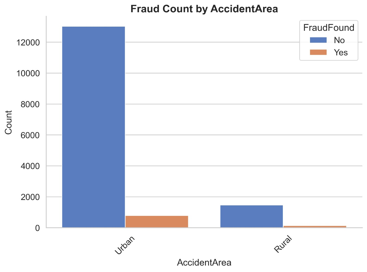
Figure 3 illustrates count distribution of fraud found or not based on marital status. It shows that there are 4510 non-fraud claims in the combined category of unmarried including single, widow and divorced while fraud claims add up to 284. In the married category, there are 9986 non-fraud claims and 639 fraud claims. It shows that married people are committing more frauds than single people. It is evident that there is not enough data in the widow and divorced categories so it makes sense to group with singles.

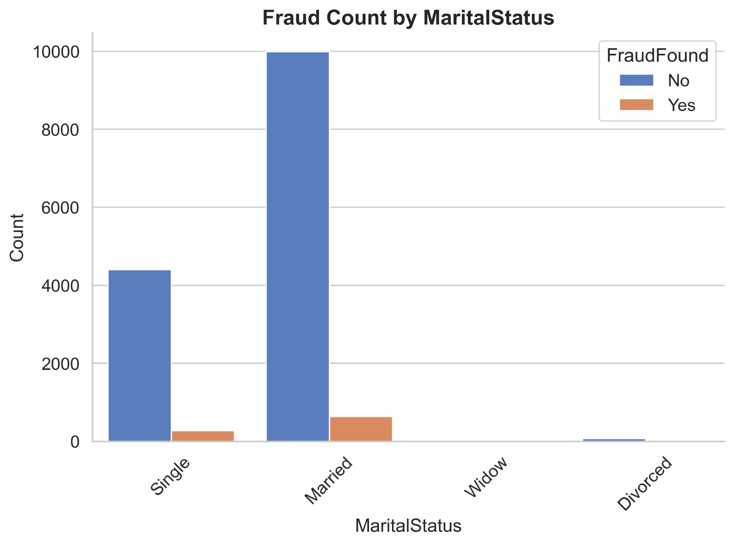
Figure 4 illustrates the count distribution of fraud found or not based on the number of cars. It appears that in 1 vehicle category there are 13465 non-fraud claims and 850 fraud claims. In the 2 vehicle category, there are 666 non-fraud claims and 43 fraud claims. In the 3 to 4 vehicle category, there are 343 non-fraud claims and 29 fraud claims. Lastly in the 5 + vehicle category, there are a total of 22 non-fraud claims and 1 fraud claim. This shows a huge imbalance in the vehicle categories where there are a lot of 1 vehicle claims and insurance claims drastically reduces when the number of cars increases.

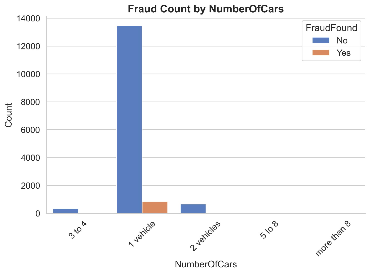
Figure 5 illustrates the count distribution of fraud found or not based on car’s make. It appears that the maximum contribution of claims are from Honda, Toyota, Chevrolet, Pontiac, Mazda and Ford. The detailed breakdown of them is : Non-fraud claims of Toyota are 2935 and fraud claims are 186, Non-fraud claims of Honda are 2621 and fraud claims are 179, Non-fraud claims of Pontiac are 3624 and fraud claims are 213, Non-fraud claims of Mazda are 2231 and fraud claims are 123, Non-fraud claims of Chevrolet are 1587 and fraud claims are 94. Non-fraud claims of Ford are 417 and fraud claims are 33. While non fraud claims from others total up to 1498 claims and fraud claims total up to 308 claims which is a very less number of claims from these many companies. It can be inferred that most of the car insurance non-fraud/fraud claims are happening in Honda, Toyota, Chevrolet, Pontiac, Mazda and Ford.

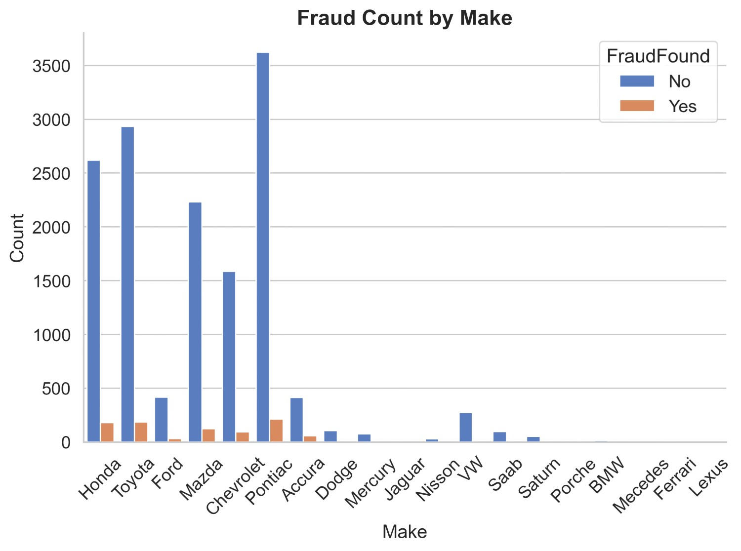
Figure 6 illustrates the count distribution of fraud found or not based on insurance agent type. It appears that in external agent non-fraud claims are 14259 and fraud claims are 919 and in internal agent non-fraud claims are 237 and fraud claims are 4. It can be inferred that people who have external agents have higher chances of committing a fraud insurance claim than people who have internal agents.

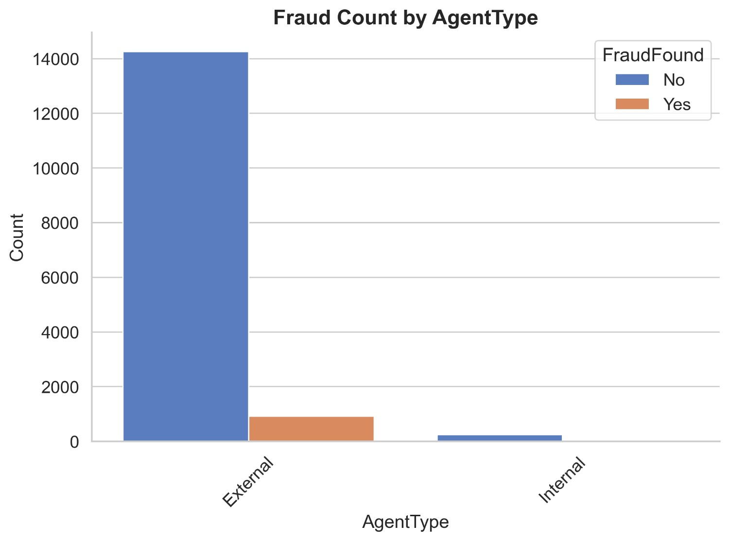
Figure 7 illustrates the count distribution of fraud found or not based on age of vehicle. It appears that most of the claims are from vehicles which are 5 years to more than 7 years old. Non fraud claims of 5 years old vehicle are 1262 and of fraud claims are 95, non-fraud claims of 6 years old vehicle are 3220 and of fraud claims are 228, non fraud claims of 7 years old vehicle are 5482 and of fraud claims are 325 and Non fraud claims of more than 7 years old vehicle are 3375 and of fraud claims are 206. While non fraud claims of vehicles less than 5 years add up to 757 and fraud claims add up to 132. It can be inferred that insurance claims of newer vehicles are not likely to be fraud as compared to vehicles aging more than 5 years.

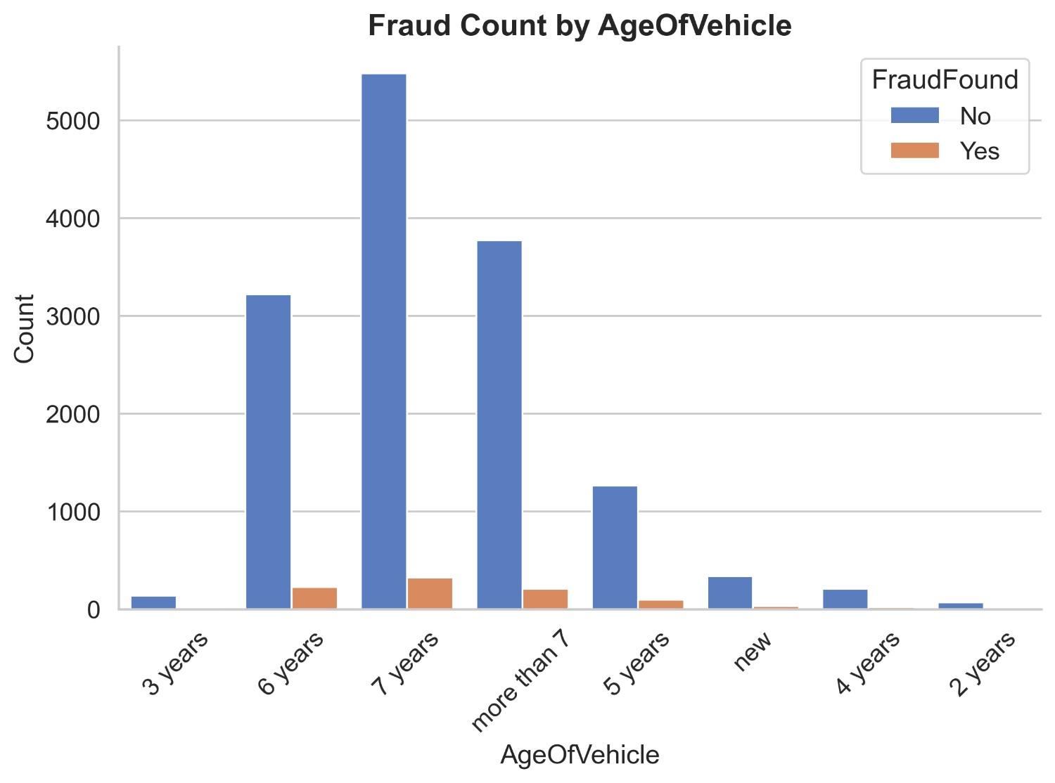
Figure 8 illustrates the count distribution of fraud found or not based on age of policyholder. It appears that most of the policyholders are from ages 31 to 65. Non fraud claims of age 31 to 35 are 5233 and fraud claims are 360, non fraud claims of age 36 to 40 are 3806 and fraud claims are 237, non fraud claims of age 41 to 50 are 2684 and fraud claims are 144 and non fraud claims of age 51 to 65 are 1322 and fraud claims are 70. While non fraud claims of ages below 30 and above 65 add up to 1451 and fraud claims are 112. It can be inferred that insurance claims which are most likely to be fraud are from ages 31 to 65.

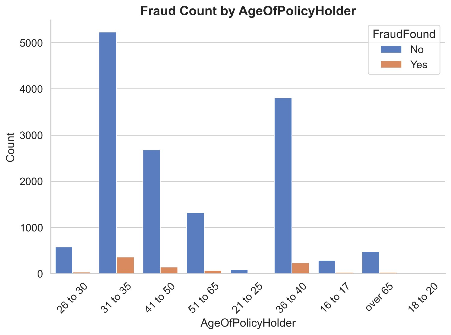
Figure 9 illustrates the count distribution of fraud found or not based on day of week claimed. It appears that most car insurances are claimed on weekdays rather than weekends by a huge difference. Non-fraud claims on weekdays are 14430 and fraud claims are 910 while non fraud claims on weekends are 166 and fraud claims are 13. It can be inferred that insurance claims are likely to be fraud on weekdays due to lack of claims on weekends. It is rare to see fraud claims made on weekends.

Figure 10 illustrates the count distribution of fraud found or not based on fault. It appears that more claims are made through policyholders than third parties but there is a better ratio of legitimate claims made through third parties than policyholders. Non-fraud claims of policyholders are 10343 and fraud claims are 886. While non-fraud claims of third parties are 4153 and fraud claims are 37. It can be easily inferred that claims made through third-party are safer than those made through policyholders.

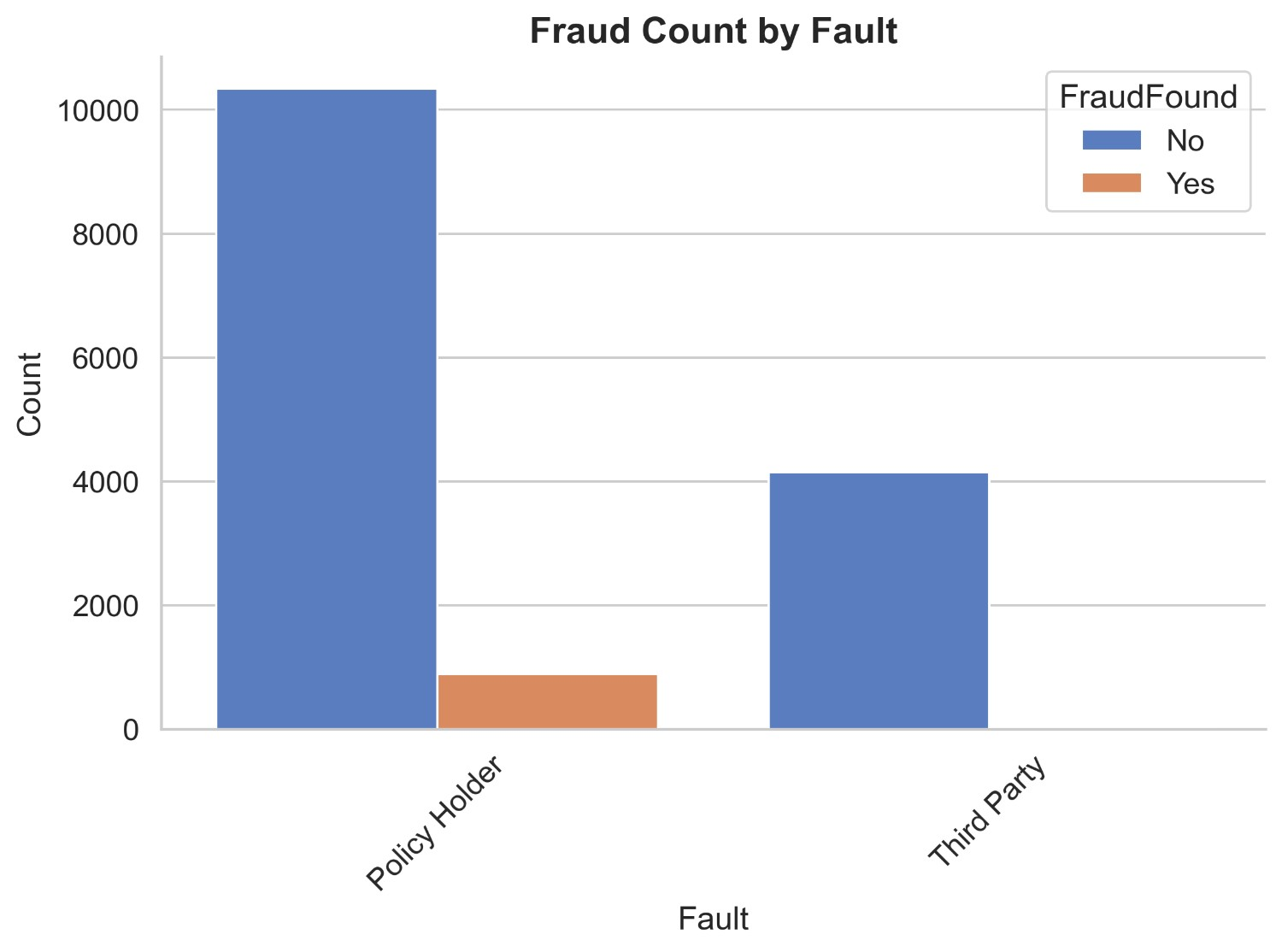
Figure 11 illustrates the count distribution of fraud found or not based on vehicle price. It appears that most insurance claims are made on vehicles priced 20k to 39k and more than 69k. Non-fraud claims of less than 20k are 993 and fraud claims are 103, non-fraud claims of 20k-29k are 7658 and fraud claims are 421, non-fraud claims of 30k-39k are 3358 and fraud claims are 175, non-fraud claims of 40k-59k are 430 and fraud claims are 31, non-fraud claims of 60k-69k are 83 and fraud claims are 4 and lastly non-fraud claims of more than 69k are 1974 and fraud claims are 189. It can be inferred that most insurance claims are from prices 20k to 39k and more than 69k having much fewer frauds compared to non-fraud indicating a better ratio than vehicles priced 20k to 39k.

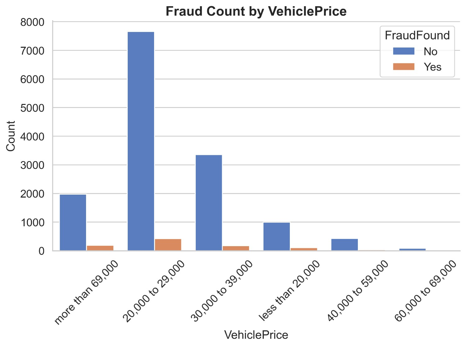
Figure 12 illustrates the count distribution of fraud found or not based on policy type. It appears that most insurance claims are being made in policy types of sedan-liability, sedan-all perils and sedan-collisions. Non-fraud claims of Sedan – Liability are 4951 and fraud claims are 36, non-fraud claims of Sedan-Collision are 5200 and fraud claims are 384 and non-fraud claims of Sedan-All Perils are 3675 and fraud claims are 411. Non-fraud claims of all policy types of utility add up to 347 and fraud claims add up to 44. Non-fraud claims of all policy types of sports add up to 323 and fraud claims add up to 48. It can be inferred that Sedan-Liability having the second highest number of fraud claims has just 36 fraud claims being the lowest indicating a legitimate, non-fraud record. Sports and Utility cars have a much lower number of claims both being legitimate and fraud. Sedan-All Perils have the least number of non-fraud claims out of all sedan policy types, yet has most number of fraud claims making it at 411 fraud claims.

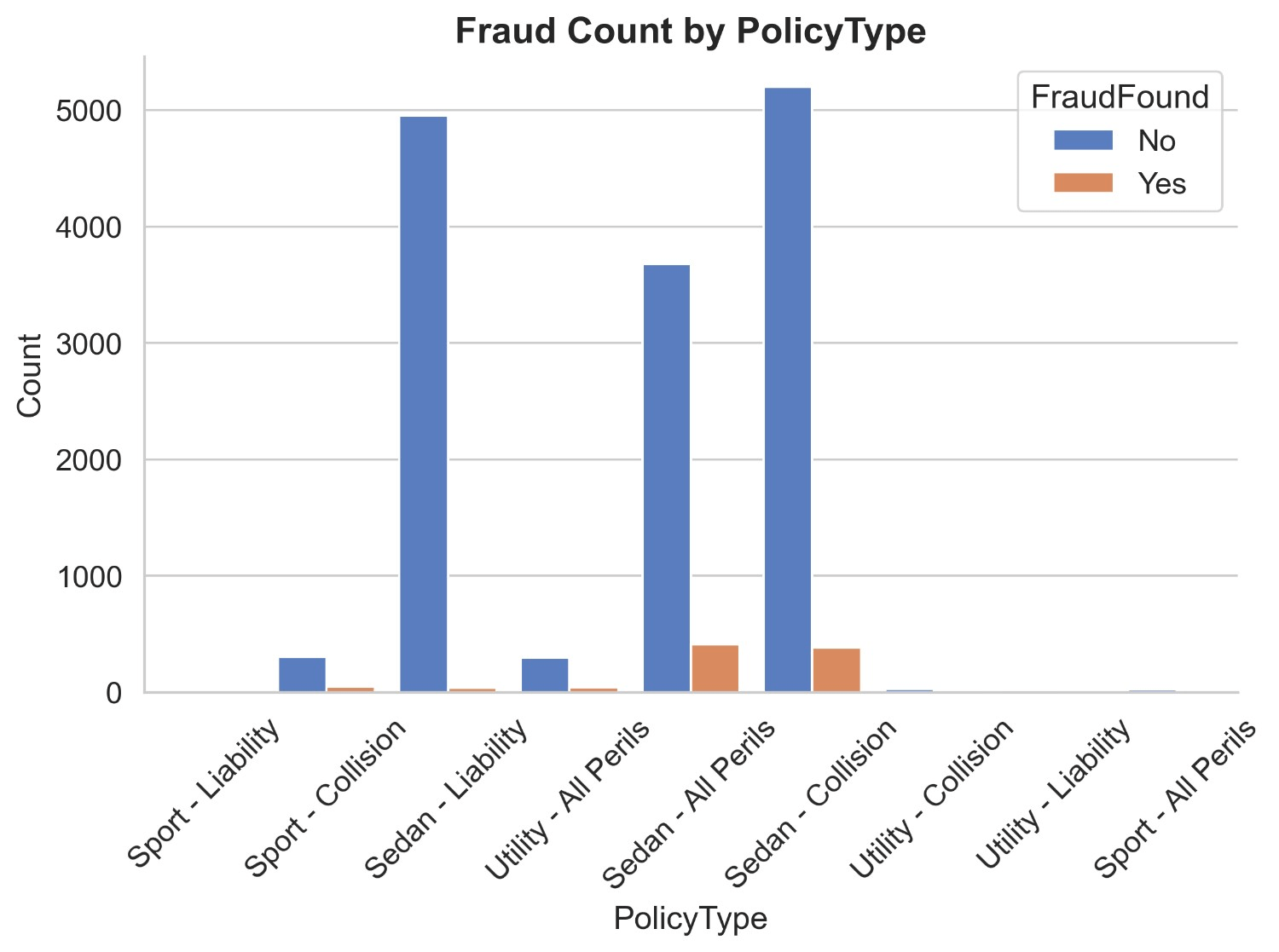
Figure 13 illustrates the count distribution of fraud found or not based on past number of claims. Non-fraud claims of none past number of claims are 4012 and fraud claims are 339, non-fraud claims of 1 past claim are 3351 and fraud claims are 222, non-fraud claims of 2 to 4 past claims are 5191 and fraud claims are 294 and non-fraud claims more than 4 claims are 1942 and fraud claims are 68.

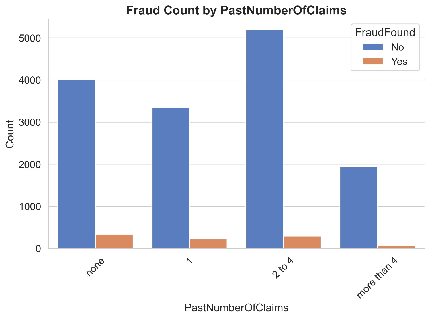
Figure 14 illustrates the count distribution of fraud found or not based on a police report filed. It appears that most of the claims are made when no police report is filed. Non-fraud claims of no police report filed are 14084 and fraud claims are 412 while non-fraud claims of police report filed are 907 and fraud claims are 16. It can be inferred that it is most likely a claim is fraud when no police report is filed.

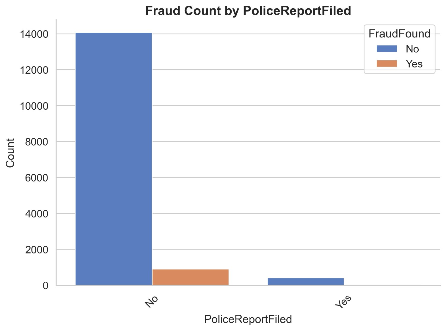
Figure 15 illustrates the count distribution of fraud found or not based on vehicle category. It appears that most claims are made of sedans and sports. Non-fraud claims of the sedan are 8875 and fraud claims are 795, non-fraud claims of sports are 5274 and fraud claims are 84 and non-fraud claims of utility are 347 and fraud claims are 44. It can be inferred that most fraud/legit claims are from sedans and also sport car claims are very less likely to be fraud.

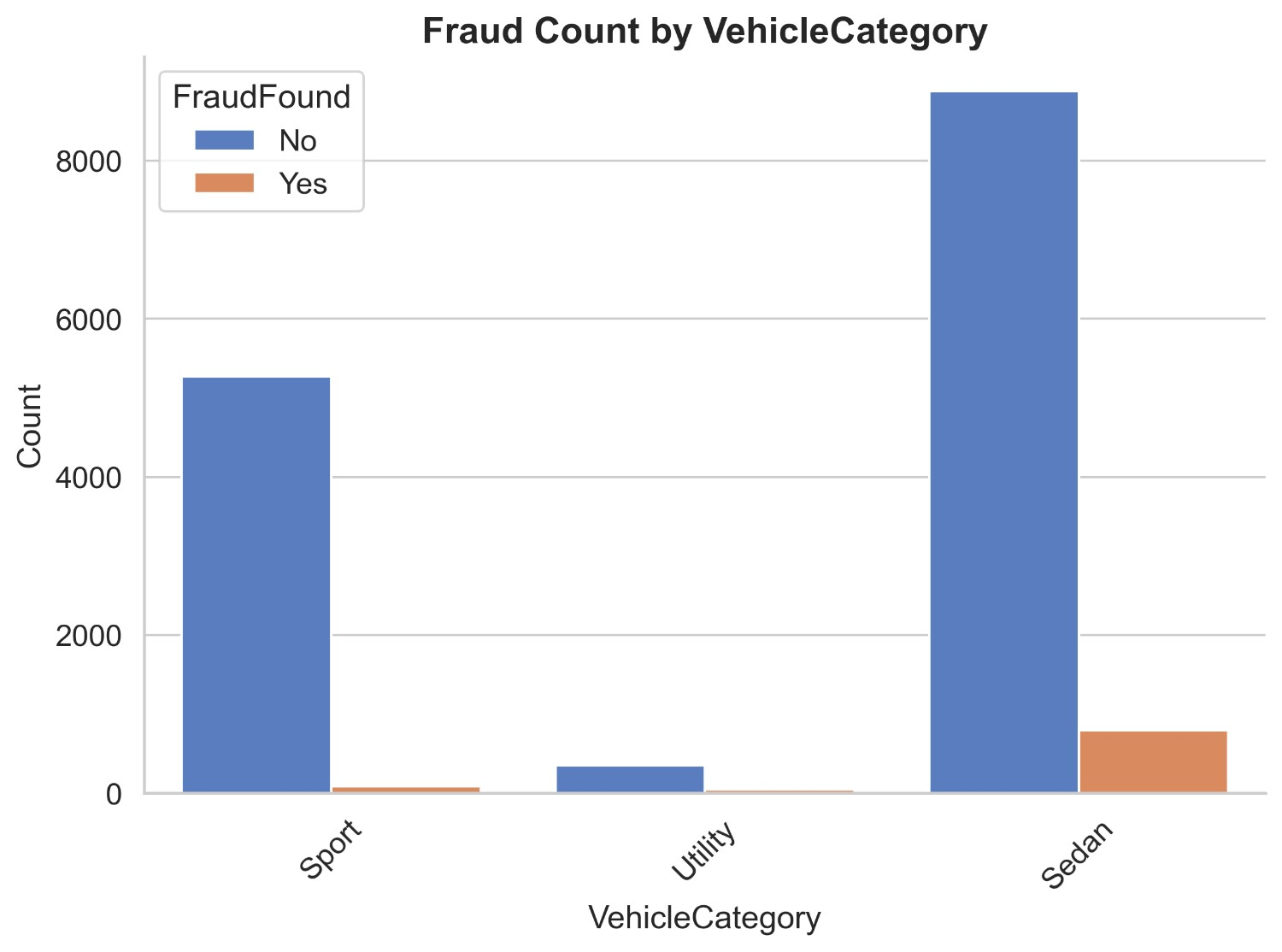
Figure 16 illustrates the count distribution of fraud found or not based on witness present. It appears that majority claims are made when no witness is present. Non-fraud claims when witness is not present are 14412 and fraud claims are 920 while non-fraud claims when witness is present are 84 and fraud claims are 3. It can be inferred that it is rare a fake car insurance claim is made when a witness is present and many claims legitimate or not are made when no witness is present as no one is there to validate the legitimacy of the claim.

Methodology

Data Preprocessing

The dataset has numerous categorical features requiring numeric transformation. The algorithm of the models need numeric values to perform their operations on. Hence comes encoding which achieves this conversion. In this section of the paper, we go through all the encoding of the factors which is the first step of data preprocessing.

Binary Encoding is a technique for converting categorical (non-numeric) data which can be classified into 2 categories into a binary (0s and 1s) format so it can be used by machine learning models. In this dataset the following features are binary encoded – Accident Area, Marital Status, Sex, Fault, Police Report Filed, Witness Present, AgentType, FraudFound and DayOfWeekClaimed as shown in Table 1. Ordinal Encoding is a technique for converting categorical (non-numeric) data which can be classified based on ranks. In this dataset the following features are ordinally encoded – Month, MonthClaimed, PastNumberOfClaims, AgeOfVehicle, AgeOfPolicyHolder, Number Of Supplements, AddressChange-Claim and NumberOfCars as shown in Table 1.

One-hot encoding is a method used to convert categorical data into a numerical format suitable for machine learning algorithms. It creates a new binary column for each unique category, where only one column is marked with a 1 (hot) to indicate the presence of a specific category, and the rest are set to 0. This avoids any ordinal relationship between categories. One-hot encoding is very useful when categories have a lot of unique values. In this dataset the following features are one hot encoded – Make, PolicyType, VehicleCategory, VehiclePrice, Days:Policy-Accident, Days:Policy-Claim and BasePolicy as shown in Table 1.

Categorical Feature	Subcategories	Encoding
Accident Area	Urban = 0, Rural = 1	Binary
Marital Status	Single, Widowed, Divorced = 0, Married = 1
Sex	Male = 0, Female = 1
Fault	Policy Holder = 0, Third Party = 1
Police Report Filed	No = 0, Yes = 1
Witness Present	No = 0, Yes = 1
Agent Type	External = 0, Internal = 1
Fraud Found	No = 0, Yes = 1
Day of Week Claimed	Weekdays are Mon, Tue,Wed, Thur, Fri = 0, Weekend is Sat and Sun
Month	Jan, Feb, Mar, Apr, May, Jun, Jul, Aug, Sep, Oct, Nov, Dec	Ordinal
Month Claimed	Jan, Feb, Mar, Apr, May, Jun, Jul, Aug, Sep, Oct, Nov, Dec
Past Number of Claims	None, 1, 2-4, More than 4
Age of Vehicle	New, 2 years, 3 years, 4 years, 5 years, 6 years, 7 years, More than 7 years
Age of Policyholder	16-17, 18-20, 21-25, 26-30, 31-35, 36-40, 36-40, 41-50, 51-65, Over 65
Number of Supplements	None, 1-2, 3-5, more than 5
Address Change Claim	No change, Under 6 months, 1 year, 2-3 years, 4-8 years
Number of Cars	1 vehicle, 2 vehicles, 3-4, 5-8, more than 8
Make	Accura, Honda, BMW Chevrolet, Ford, Dodge, Ferrari, Jaguar, Lexus, Mazda, Mercedes, Nisson, Pontiac, Porsche, Saab, Saturn, Toyota, VW	One-Hot
PolicyType	Sedan All Perils, Sedan Collision, Sedan Liability, Sport All Perils, Sport Collision, Sport Liability, Utility All Perils, Utility Collision, Utility Liability
Vehicle Category	Sedan, Utility, Sport
Vehicle Price	20-29 k, 30-39 k, 40-59 k, 60-69 k, Less than 20k, More than 69k
Days Policy Accident	None, 1 to 7, 8 to 15, 15 to 30, More than 30
Days Policy Claim	8 to 15, 15 to 30, More than 30
Base Policy	All Perils, Collision, Liability

Models and Evaluation Metrics

The dataset is split into training and testing subsets using an 80/20 ratio, where 80% of the data is used to train the model and the remaining 20% is reserved for evaluating its performance on unseen examples. Because the classes are imbalanced, we apply a stratified split so that both the training and test sets preserve the original class proportions. This helps prevent the model from overfitting to the majority class during training and ensures that evaluation metrics on the test set reflect real-world class frequencies.

Models used in this study were Logistic Regression model, KNN model, Decision Tree model, Random Forest model and XGBoost model. Logistic regression is a model is a classification algorithm used to predict the probability of a binary outcome. Its pros are it is simple and interpretable, fast and efficient and works well with linearly separable data while its cons are it requires scaling of features, does not perform well for complex datasets and works well only with binary analysis Horton et al. (2001)¹⁵.

K-Nearest Neighbors (KNN) is a non-parametric, instance-based machine learning algorithm used for classification and regression. Its pros are it requires no training step, simple to implement and adapts well with dataset while its cons are it becomes slow with large dataset, memory intensive as it needs to store entire training data and its performance drops with high dimensional data. GeeksforGeeks (2024)¹⁶ Random Forest is an ensemble learning method that builds multiple decision trees and combines their outputs to improve prediction accuracy and reduce overfitting. Its pros are it is highly accurate, handles large and high dimension datasets and reduces overfitting while its cons are it is less interpretable than a single tree, uses large memory and it is slow. Bulagang et al. (2021)¹⁷.

XGBoost (Extreme Gradient Boosting) is a powerful, scalable, and efficient implementation of the Gradient Boosting algorithm. It’s used for classification, regression, and ranking problems. Its pros are its performance is high, fast and efficient and handles missing values while its cons are it is complex and harder to tune, less interpretable and it trains slowly on large datasets. Khan et al. (2024)¹⁸.

To evaluate the performance of the models, we used train and test precision, recall and f1 score metrics. Precision is the proportion of predicted positive cases that are actually correct. Precision = (True Positives) /(True Positives + False Positives). High precision means few false positives and more true positives. Recall is the proportion of actual positive cases that were correctly predicted. Recall = (True Positives) /(True Positives + False Negatives). High recall means few false negatives. F1-score is the harmonic mean of precision and recall. F1-score = 2 X (Precision X Recall) / (Precision + Recall). It balances precision and recall and it is useful when there is imbalance between classes. PR-AUC (Precision-Recall Area Under the Curve) summarizes the trade-off between precision and recall across different threshold values; a higher PR-AUC indicates better performance in distinguishing positive and negative classes, especially in imbalanced datasets.

Overfitting leads to a model that performs well during training but poorly in testing. Using test performance and metrics like precision, recall, and F1-score ensures that the model is not just accurate, but also reliable and predictive. A good fit model includes high training accuracy with high test accuracy, overfitting includes high training accuracy with low test accuracy and underfitting includes low training accuracy with low test accuracy.

Hyperparameter Tuning

Hyperparameter tuning of a model is the process of finding the best combination of hyperparameters for a machine learning model to improve its performance. Grid search is a hyperparameter tuning technique that tries all possible combinations of the hyperparameters and gives the combination which gives the best model performance Scikit-learn (2024)¹⁹. During hyperparameter tuning, we apply 3-fold stratified cross-validation on the training split using GridSearchCV. At each iteration, the training data is partitioned into three stratified folds that preserve the original class proportions; the model is trained on one fold and validated on the other, then the roles are swapped in the next iteration. Performance is averaged across folds to robustly estimate generalization and select the best hyperparameters. This procedure is confined to the training data to avoid information leakage, after which the final model is to refit on the full training set and evaluate once on the held-out test set.

As baselines, we trained Logistic Regression and k-Nearest Neighbors using their default hyperparameters (applying feature scaling for KNN to ensure distance computations are meaningful). These uncomplicated setups provide a transparent reference point for model capacity and data separability without the confounding effects of extensive tuning. Comparing their results to hyperparameter ensemble based models highlights the incremental value of non-linear decision boundaries and built-in feature interactions, making any performance gains from the tree-based approaches clear and attributable.

In this study, following parameters of the XGBoost model were tuned : n_estimators, lambda, alpha, scale_pos_weights, subsample, learning_rate and colsample_bytree as shown in Table 2. n_estimators tells the number of trees to be built in the model (i.e., boosting rounds), lambda includes L2 regularization term on weights to prevent overfitting, alpha includes L1 regularization term on weights to encourage sparsity, scale_pos_weight balances positive and negative classes, useful for imbalanced datasets, subsample are fractions of training data used for each boosting round to prevent overfitting, learning_rate shrinks the contribution of each tree to make learning more robust (also called eta) and colsample_bytree is fraction of features randomly sampled for each tree to reduce overfitting. Range of n_estimators is [50,100], learning_rate is [0.01,0.05,0.1,0.2,0.3], subsample is [0.5,0.6,0.7,0.8,0.9], colsample_bytree is [0.5,0.6,0.7,0.8,0.9], lambda is [0,0.01,0.1,1,10], alpha is [0,0.01,0.1,1,10] and scale_pos_weight is [1, 10, 50, 100].

In this study, following parameters of the Random Forest model were tuned : n_estimators, min_samples_split, max_features and class_weight as shown in Table 2. min_samples_split is the minimum number of samples required to split an internal node, max_features is the maximum number of features to consider when looking for the best split and class_weight assigns weights to classes to handle imbalanced data. The range of n_estimators is [100,500], min_samples_split is range(50,100,10), max_features is range(10,70,5) and class_weight is balanced.

Model	Parameter	Range
XGBoost	n_estimators	[50,100]
	learning_rate	[0.01,0.05,0.1,0.2,0.3]
	subsample	[0.5,0.6,0.7,0.8,0.9]
	colsample_bytree	[0.5,0.6,0.7,0.8,0.9]
	lambda	[0,0.01,0.1,1,10]
	alpha	[0,0.01,0.1,1,10]
	scale_pos_weight	[1, 10, 50, 100]
Random Forest	n_estimators	[100,500]
	min_samples_split	(50,100,10)
	max_features	(10,70,5)

Handling Data Imbalance

To mitigate the data imbalance, we explored different techniques such as class weight balancing, undersampling and oversampling + undersampling. Using class weights with the original dataset is a technique to handle class imbalance without modifying the data itself. Instead of generating new samples or duplicating existing ones, you assign more importance (weight) to the minority class during model training. This means the model will treat mistakes on the minority class as more costly than those on the majority class. As a result, it becomes more sensitive to the underrepresented class, improving its ability to predict it correctly. This approach keeps the data distribution unchanged, is efficient, and reduces the risk of overfitting.

Undersampling is a technique used to handle imbalanced datasets by reducing the number of samples in the majority class so that it becomes more balanced with the minority class. This technique is used when the model is biased towards the majority class due to the large number of majority class as compared to minority class. Its accuracy is very low for minority classes.

Oversampling + Undersampling is a technique used to handle imbalanced datasets by increasing the number of minority classes and reducing the number of majority classes till both of them are equal. SMOTE (Synthetic Minority Over-sampling Technique) is a method used to handle imbalanced datasets by creating synthetic examples of the minority class rather than simply duplicating them Swastik (2020)²⁰. ADASYN (Adaptive Synthetic Sampling) is an extension of SMOTE that focuses on generating more synthetic samples for minority class instances that are harder to learn, based on the density distribution of the data. This helps the model pay more attention to complex or ambiguous regions in the dataset He et al. (2008)²¹ In our study, we implemented and compared both SMOTE and ADASYN to evaluate which method resulted in better model performance.

Feature Importance Analysis

We are doing feature importance analysis to understand how different features affect the model’s prediction on fraud and non-fraud claims. Feature importance analysis aims to identify which input features have the most influence on a machine learning model’s predictions. This helps improve model interpretability, aids in feature selection, and allows us to understand what factors are driving outcomes. By highlighting the most relevant features, it can also improve model performance, reduce overfitting, and guide decisions in critical fields like healthcare, finance, and policy.

One powerful method for feature importance analysis is SHAP (SHapley Additive exPlanations), which is based on cooperative game theory. SHAP assigns each feature an importance value for a particular prediction by calculating how much each feature contributes, on average, to the change in model output across all possible combinations of features. Unlike simpler methods, SHAP provides local explanations (per prediction) as well as global insights (overall feature impact), offering a comprehensive view of model behavior Lundberg et al. (2017)²².

Results and Discussion

We are presenting the results of original imbalance data with balanced class weights then undersampled and lastly of the oversampled data. Table 3 results compare three models – Logistic Regression, XGBoost, and Random Forest on their ability to detect fraud (the minority class) versus non-fraud(majority class). Across all models, performance on the “Not Fraud” class is consistently high in terms of precision, recall, and F1-score for both training and test sets. However, significant differences arise in detecting “Fraud”, which is much harder due to class imbalance.

Logistic Regression and KNN perform poorly on the fraud class, showing 0.00 F1-scores on test data, indicating they fail to correctly identify fraud cases. XGBoost shows improved performance, especially in training (F1 = 0.93) with its precision of 0.98 and recall of 0.88, but its fraud detection drops significantly on the test set (F1 = 0.50) with its precision of 0.78 and recall of 0.37. The Random Forest model shows the best generalization, with a Fraud class test F1-score of 0.46, maintaining a balance between precision (0.35) and recall (0.70). This suggests that class balancing and hyperparameter tuning in Random Forest helped the model better generalize fraud detection without severely sacrificing accuracy on the majority class. In terms of PR-AUC, which evaluates the trade-off between precision and recall across thresholds, Logistic Regression achieved a very low score of 0.162, indicating poor discrimination of the fraud class. Random Forest improved moderately with a PR-AUC of 0.454, while XGBoost achieved the highest PR-AUC of 0.675, showing its superior ability to distinguish between fraudulent and non-fraudulent cases. Overall, the results highlight the challenge of fraud detection in original data with no sampling technique.

Model	Train/Test	Label	Precision	Recall	F1	ROC- AUC	PR- AUC	Samples
Logistic Regression	Train	Not Fraud	0.94	1.00	0.97	0.80	0.162	11597
		Fraud	0.00	0.00	0.00			738
	Test	Not Fraud	0.94	1.00	0.97			2889
		Fraud	0.00	0.00	0.00			185
XGBoost ‘alpha’: 0.1, ‘colsample_bytree’: 0.8, ‘lambda’: 0, ‘learning_rate’: 0.3, ‘n_estimators’: 50, ‘scale_pos_weight’: 1, ‘subsample’: 0.9	Train	Not Fraud	0.99	1.00	1.00	0.971	0.675	11597
		Fraud	0.98	0.88	0.93			738
	Test	Not Fraud	0.96	0.99	0.98			2889
		Fraud	0.78	0.37	0.50			185
Random Forest ‘class_weight’: ‘balanced’, ‘max_features’: 40, ‘min_samples_split’: 50, ‘n_estimators’: 100	Train	Not Fraud	1.00	0.94	0.97	0.926	0.454	11597
		Fraud	0.50	0.96	0.65			738
	Test	Not Fraud	0.98	0.92	0.95			2889
		Fraud	0.35	0.70	0.46			185

Table 4 presents the comparison of three models – Logistic Regression, XGBoost Model and Random Forest Model based on precision, recall, and F1 scores for fraud detection reveals notable differences in performance between algorithms and across training and test sets. Logistic Regression shows moderately balanced performance, with a fraud recall of 0.88 on the training set but a significant drop to 0.67 on the test set, suggesting potential overfitting. KNN performs worst overall, with low precision and recall on both training and test sets for the fraud class (test F1 score of only 0.48), indicating its ineffectiveness in capturing patterns of fraudulent claims. Based on PR-AUC scores, Logistic Regression achieved 0.718, Random Forest 0.8, and XGBoost 0.791, indicating that while all three models were able to learn meaningful discrimination after undersampling, Random Forest demonstrated the highest PR-AUC score. XGBoost also performed competitively, whereas Logistic Regression scored comparatively less.
XGBoost and Random Forest outperform the others in terms of generalization and fraud detection. XGBoost, using tuned hyperparameters, achieves strong recall (0.94), precision (0.70) and f1 score (0.80) for fraud in the test set, suggesting it effectively identifies fraudulent claims without too many false positives. The Random Forest model, with a high number of estimators and balanced class weights, yields consistent and robust performance, achieving a fraud F1 score of 0.80 on the test set same as XGBoost model. Overall, tree-based ensemble methods (XGBoost and Random Forest) significantly outperform linear and distance-based classifiers in detecting fraudulent car insurance claims.

Model	Train/Test	Label	Precision	Recall	F1	ROC- AUC	PR- AUC	Samples
Logistic Regression	Train	Not Fraud	0.84	0.64	0.73	0.766	0.718	738
		Fraud	0.71	0.88	0.79			738
	Test	Not Fraud	0.78	0.59	0.67			185
		Fraud	0.67	0.83	0.74			185
XGBoost ‘alpha’: 1, ‘colsample_bytree’: 0.6, ‘lambda’: 0.01, ‘learning_rate’: 0.01, ‘n_estimators’: 100, ‘subsample’: 0.9	Train	Not Fraud	0.93	0.67	0.78	0.822	0.791	738
		Fraud	0.74	0.95	0.83			738
	Test	Not Fraud	0.91	0.59	0.72			185
		Fraud	0.70	0.94	0.80			185
Random Forest ‘class_weight’: ‘balanced’, ‘max_features’: 60, ‘min_samples_split’: 50, ‘n_estimators’: 500	Train	Not Fraud	0.94	0.67	0.78	0.83	0.8	738
		Fraud	0.74	0.96	0.84			738
	Test	Not Fraud	0.91	0.60	0.72			185
		Fraud	0.70	0.94	0.80			185

Table 5 results compare three models – Logistic Regression, XGBoost, and Random Forest show better balance between detecting fraud and non-fraud compared to the original data. Logistic Regression demonstrates decent generalization with a Fraud class test F1-score of 0.20, though it struggles with recall (0.16), indicating it misses many actual fraud cases. The KNN model performs better on training data but suffers on the test set, especially for “Not Fraud” (F1 = 0.77) and “Fraud” (F1 = 0.28), suggesting possible overfitting. In terms of PR-AUC, all three models achieved relatively low scores, with Logistic Regression obtaining the lowest PR-AUC of 0.254, Random Forest achieving the highest PR-AUC of 0.378, and XGBoost attaining a moderate PR-AUC of 0.343.

XGBoost delivers high training scores, nearly perfect for both classes, but its performance drops on the test set especially for fraud detection (F1 = 0.28), precision of 0.35 and recall of 0.24 reflecting some overfitting. Still, its overall precision and recall are higher than the simpler models. Random Forest stands out with the highest Fraud class F1-score on the test set (0.34), showing a better balance between precision (0.43) and recall (0.29). It also maintains strong “Not Fraud” classification. This suggests that its handling of class imbalance(class weight = balanced) and tuned hyperparameters allow it to generalize best to unseen data, especially for the fraud detection class.

Model	Train/Test	Label	Precision	Recall	F1	ROC- AUC	PR- AUC	Samples
Logistic Regression	Train	Not Fraud	0.86	0.95	0.90	0.777	0.254	5798
		Fraud	0.94	0.85	0.89			5798
	Test	Not Fraud	0.90	0.94	0.92			1450
		Fraud	0.27	0.16	0.20			185
XGBoost ‘alpha’: 0.01, ‘colsample_bytree’: 0.8, ‘lambda’: 0.01, ‘learning_rate’: 0.3, ‘n_estimators’: 100, ‘subsample’: 0.8	Train	Not Fraud	0.99	0.99	0.99	0.822	0.343	5798
		Fraud	0.99	0.98	0.99			5798
	Test	Not Fraud	0.91	0.94	0.92			1450
		Fraud	0.35	0.24	0.28			185
Random Forest ‘class_weight’: ‘balanced’, ‘max_features’: 40, ‘min_samples_split’: 50, ‘n_estimators’: 100	Train	Not Fraud	0.92	0.97	0.94	0.822	0.378	5798
		Fraud	0.97	0.92	0.94			5798
	Test	Not Fraud	0.91	0.95	0.93			1450
		Fraud	0.43	0.29	0.34			185

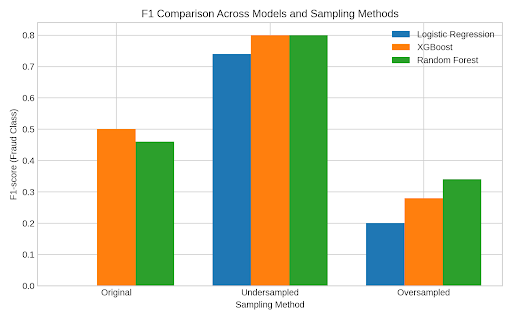
The results across all three sampling strategies (Figure 17), original imbalanced data with balance class weights, undersampling, and oversampling, demonstrate the critical impact of data distribution on fraud detection model performance. Random Forest and XGBoost consistently outperformed linear (Logistic Regression) and distance-based (KNN) classifiers, particularly in identifying the minority class (fraud). However, their performance varied significantly depending on the sampling method. In the original imbalanced dataset with balanced class weights, all models except Random Forest and XGBoost performed poorly on fraud detection, with Logistic Regression and KNN failing entirely (F1 = 0.00). This highlights the severe limitations of using imbalanced data without proper sampling strategies, as models tend to become biased toward the majority class.

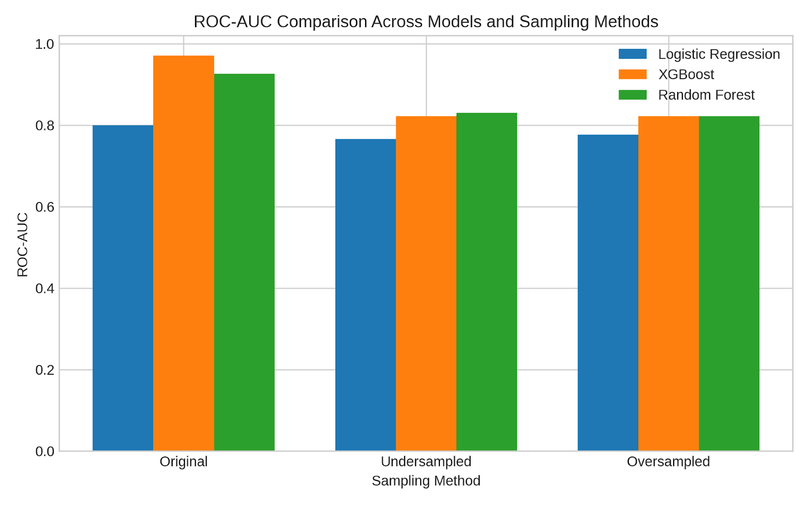
Both Random Forest and XGBoost demonstrated competitive and relatively strong ROC-AUC (Figure 18) and PR-AUC (Figure 19) scores, indicating their effectiveness in distinguishing between fraudulent and non-fraudulent transactions. In contrast, Logistic Regression consistently recorded the lowest ROC-AUC and PR-AUC scores across all sampling strategies, suggesting that it struggles to accurately identify fraud cases with reliable precision and recall. Among the sampling methods, the original imbalanced dataset yielded the highest ROC-AUC values, while undersampling produced the best PR-AUC results across all models, highlighting the trade-off between overall discrimination and minority-class detection.

Among the sampling strategies, undersampling combined yielded the best overall performance. Both XGBoost and Random Forest achieved the highest fraud F1-scores (0.80) in the test set under undersampling, maintaining a balance between precision and recall. This indicates that reducing the majority class to match the minority class size helps models better learn fraudulent patterns without being overwhelmed by non-fraud data. On the other hand, oversampling using SMOTE improved training scores significantly but led to overfitting, especially in XGBoost, where the fraud F1-score dropped to 0.28 on the test set despite near-perfect training performance. KNN again underperformed across all sampling methods, reinforcing that it struggles with imbalanced, high-dimensional data.

Table 6 compares Logistic Regression, XGBoost, and Random Forest after applying SMOTE and ADASYN. This table summarises the results of the experiment which compared two oversampling techniques SMOTE and ADASYN. Logistic Regression showed low recall (0.10–0.16) and modest precision (~0.25), resulting in poor F1-scores. XGBoost performed slightly better, with SMOTE giving the highest F1 (0.28) and stable ROC-AUC (≈0.83). Random Forest benefited most from oversampling, achieving high recall (0.54) and the best F1 (0.34) with consistent ROC-AUC (0.822-0.85). This reports test metrics for fraud labels only because we do well for non-fraud results. Overall, oversampling had limited effect on Logistic Regression and XGBoost but relatively better on Random Forest’s detection of the fraud class.

Model	SMOTE/ ADAYSN	Precision	Recall	F1	ROC- AUC	PR- AUC
Logistic Regression	SMOTE ADAYSN	0.27 0.23	0.16 0.10	0.20 0.14	0.777 0.776	0.254 0.157
XGBoost	SMOTE ADAYSN	0.35 0.32	0.24 0.14	0.28 0.19	0.822 0.842	0.343 0.233
Random Forest	SMOTE ADAYSN	0.43 0.21	0.29 0.54	0.34 0.31	0.822 0.85	0.378 0.229

Analysis of misclassified cases from our best model, XGBoost, showed strong overall detection performance, with limited misclassifications. On the test set ( cases), the model produced 116 false negatives (missed frauds) and 20 false positives (legitimate claims flagged), corresponding to 0.7% and 5.5% of the test set, respectively. When scaled to the full dataset, this equates to roughly 105 missed frauds and 850 over-flagged legitimate claims out of 15,419 total. These results indicate that most fraudulent claims were successfully identified, though a small number of legitimate claims were misclassified due to overlapping feature patterns.

The work by Wang et al. (2018), which focused on integrating LDA topic modeling with a deep neural network (DNN) for fraud detection, distinguishes itself by offering a more comprehensive and transparent evaluation of model performance under high class imbalance. While Wang and Xu achieved high overall metrics (accuracy of 91.4%, F1-score of 91.3%), their evaluation was based on averaged metrics that do not reflect the model’s effectiveness in detecting fraudulent claims specifically-an issue in datasets where fraud cases (minority class) are significantly underrepresented. In contrast, the current study provides class-specific metrics (precision, recall, F1) for both fraud and non-fraud classes across different models and sampling strategies, revealing how techniques like undersampling and SMOTE impact fraud detection.

To validate whether performance differences between models were statistically significant rather than incidental, we conducted paired t-tests on F1 and ROC-AUC across 3-fold cross-validation.

Table 7 presents the pairwise McNemar p-values comparing the accuracy of Logistic Regression, Random Forest, and XGBoost models (with class weighting) on the test data. The results indicate that the difference in accuracy between Logistic Regression and Random Forest (p = 0.006982) is statistically significant at the 0.05 level, suggesting that these models perform differently. Similarly, the difference between Random Forest and XGBoost (p = 0.006982) is also significant. However, the comparison between Logistic Regression and XGBoost shows no significant difference (p = NaN, implying no measurable or comparable variation). Overall, these results suggest that Random Forest differs significantly from both Logistic Regression and XGBoost in classification accuracy, while Logistic Regression and XGBoost exhibit similar performance, indicating that the observed differences are statistically meaningful rather than incidental.

Logistic Reg
Random Forest	0.006982
Xgboost	NaN	0.006982
	Logistic Reg	Random Forest	Xgboost

To better understand how individual features influence model predictions and to ensure transparency in the decision-making process, interpretability techniques were explored in this study. Lundberg et al. (2017)²² introduced SHAP (SHapley Additive exPlanations) as a unified, theoretically grounded approach for interpreting machine learning models through additive feature attributions. Unlike wrapper-based feature selection methods such as Boruta, SHAP provides consistent and locally accurate estimates of each feature’s contribution to individual predictions. Its model-agnostic design enables interpretation across complex models like Random Forest and XGBoost, offering richer explanatory insights rather than simple feature relevance. Thus, following Lundberg et al. (2017)²², SHAP was employed in this study primarily to enhance interpretability and transparency rather than to replicate feature selection experiments.

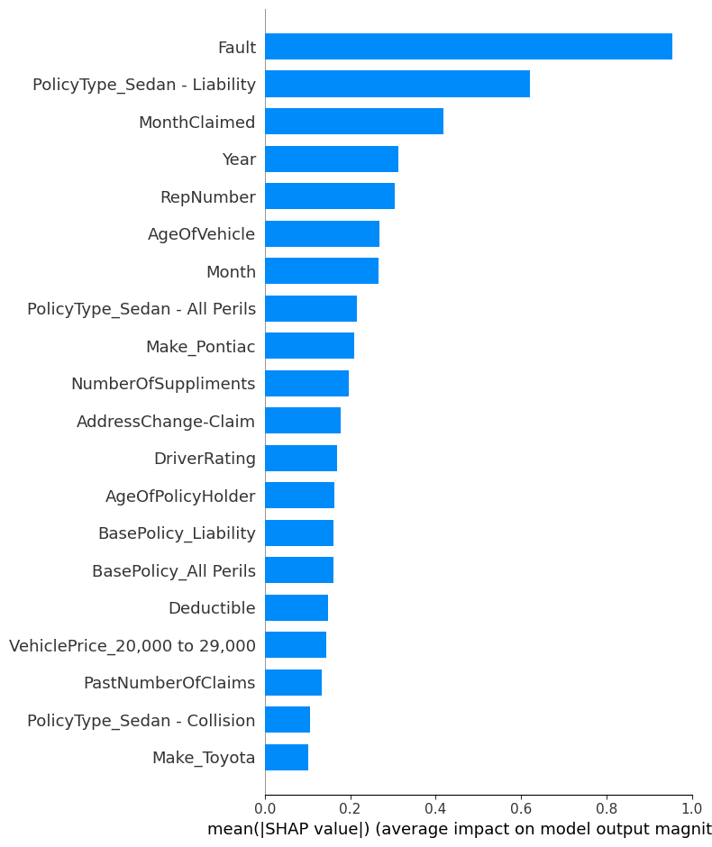
The SHAP summary plot is a key outcome of the analysis and achieves the aim of the study to identify which factors most significantly influence whether a car insurance claim is classified as fraudulent. In Figure 20, features are ranked by their importance (top to bottom), and the spread along the x-axis indicates the magnitude and direction of each feature’s impact on the model’s output. Each point represents a SHAP value for a single data instance, colored by the feature’s value (red = high, blue = low). In Figure 21, the bar plot shows the average impact of each feature on the model’s predictions and helps identify the most significant factors. The x-axis represents the mean absolute SHAP value, which quantifies the average contribution of each feature to the model’s output, regardless of direction. The higher the bar, the more influence that feature has on prediction decisions across the dataset.

Figure 20 shows that features like Fault, PolicyType_Sedan – Liability, MonthClaimed, and Year have the largest impact on predictions. For example, a high value for “Fault” pushes the model strongly toward predicting fraud, indicating it is a critical indicator. Similarly, specific policy types and time-related features (like claim month and year) also show significant influence. On the other hand, features like “Make_Toyota” or “PolicyType_Sedan – Collision” have relatively smaller impacts.

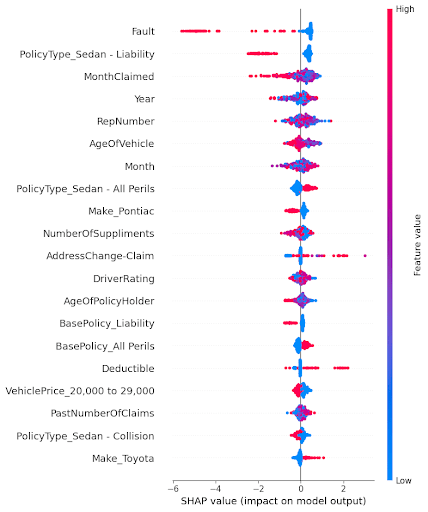
Figure 21 shows that the most impactful feature is clearly Fault, indicating that whether the claim made by the person was at fault plays the largest role in determining the likelihood of fraud. Followed by PolicyType_Sedan – Liability and MonthClaimed, suggesting that both the policy type and the timing of the claim are also strong indicators. Features like RepNumber, Year, and AgeOfVehicle also contribute meaningfully. On the other end, attributes like Make_Toyota and PolicyType_Sedan Collision have the smallest average impact.

Claims in which the policyholder is found to be at fault are often treated with greater suspicion, as insurers recognize that “staged accidents and inflated damage reports are among the most common types of auto insurance fraud” NICB (2023)²³.The type of policy also influences fraud risk: comprehensive or All Perils coverage—designed to protect against almost any cause of loss except explicit exclusions—tends to experience higher fraud incidence. According to the International Association of Insurance Supervisors, “broad or all-risk coverage provides greater opportunity for opportunistic fraud due to the wide scope of indemnifiable events” IAIS (2022)²⁴.Furthermore, the timing of claims can be indicative of suspicious behavior; empirical studies note that “seasonal spikes in claim submissions often correlate with opportunistic or organized fraud attempts” Nguyen et al. (2022)²⁵. Collectively, these factors—fault status, policy breadth, and claim timing—represent key red flags that guide insurers’ fraud detection efforts.

This study also differs from “Insurance Fraud Detection: Evidence from Artificial Intelligence and Machine Learning” by Aslam et al. (2022)² in its approach to feature importance analysis. Aslam et al. employed the Boruta algorithm for selecting significant features, identifying variables like Fault and Age of Policyholder as important. In contrast, this study uses SHAP (SHapley Additive exPlanations) values, which not only rank features by importance but also explain each feature’s direction and magnitude of impact on individual predictions. While Boruta provides a robust filter for feature selection, SHAP offers a deeper understanding and interpretability, helping to understand how and why features influence fraud predictions which makes it more suitable for real-world applications where transparency and justification for every decision are critical.

The limitation of our research is that it does not include a separate experiment on future fraud schemes, the approach is designed to be easily retrainable with updated data. Tree-based ensemble models such as Random Forest are known to be relatively robust to moderate distribution shifts, but we recommend that insurers periodically retrain the model on newly collected claims data to adapt to evolving fraud patterns and mitigate concept drift. This ensures the system remains relevant as fraud strategies change over time. It would be great to have fraud detection data over many continuous years to investigate the time drift component.

Conclusion

The primary objective of this study was to analyze and identify key factors that influence whether a car insurance claim is fraudulent or not. We aimed to build an effective yet interpretable fraud detection model that performs reliably despite the presence of significant class imbalance in the dataset. Additionally, we sought to evaluate the impact of different sampling techniques, such as class weighting, undersampling, and SMOTE(oversampling technique), on model performance and to provide detailed insights through model interpretability and feature importance analysis.

Among the various models evaluated, Logistic Regression, KNN, Random Forest, and XGBoost, the Random Forest model with undersampling emerged as the best-performing approach. It achieved the highest F1-score (0.80) for the fraud class in the test set, indicating a strong balance between precision and recall. This model was able to generalize well without overfitting and proved more effective than linear or distance-based classifiers, especially in detecting the minority class (fraudulent claims).

This study confirmed that class imbalance significantly hinders and damages fraud detection performance, particularly for minority class predictions. Models trained on the original imbalanced data showed high accuracy but failed to detect fraud cases effectively, with some models reporting an F1-score of 0.00 for the fraud class. Undersampling provided the best improvement in fraud detection, allowing models to better learn the patterns of minority class without being overwhelmed and dominated by the majority class. SMOTE enhanced training performance but introduced overfitting in some cases, especially with XGBoost which also resulted in poor performance of the model.

Lastly, using SHAP (SHapley Additive exPlanations), the study provided a transparent interpretation of how different features influenced model predictions. Features like Fault, Policy Type, and Month Claimed were found to have the most significant impact on determining whether a claim was fraudulent. SHAP not only identified important features but also explained the direction and extent of their influence on each prediction, enhancing the interpretability of the model. This level of insight is crucial for stakeholders to understand, trust, and act on the model’s decisions in real-world insurance fraud detection scenarios.

References

1. L. Ding, A. Sharma, and S. Verma. Global trends and challenges in insurance fraud detection Journal of Risk and Financial Analytics. 18(1) 45–62, 2024. https://doi.org/10.1016/j.jrfa.2024.01.005 [↩]
2. Aslam, F., Ajaz, T., & Rahman, M. U. (2022). Insurance fraud detection: Evidence from artificial intelligence and machine learning. Research in International Business and Finance, 62, 101744. https://doi.org/10.1016/j.ribaf.2022.101744 [↩] [↩]
3. Wang, Y., & Xu, W. (2018). Leveraging deep learning with LDA-based text analytics to detect automobile insurance fraud. Decision Support Systems, 105, 87–95. https://doi.org/10.1016/j.dss.2017.11.005 [↩]
4. Chawla, N. V., Bowyer, K. W., Hall, L. O., & Kegelmeyer, W. P. (2002). SMOTE: Synthetic minority over-sampling technique. Journal of Artificial Intelligence Research, 16, 321–357. https://doi.org/10.1613/jair.953 [↩]
5. Chawla, N. V., Lazarevic, A., Hall, L. O., & Bowyer, K. W. (2003). SMOTEBoost: Improving prediction of the minority class in boosting. In PKDD 2003 (pp. 107–119). Springer. https://doi.org/10.1007/978-3-540-39804-2_12 [↩]
6. Batista, G. E. A. P. A., Prati, R. C., & Monard, M. C. (2004). A study of the behavior of several methods for balancing machine learning training data. SIGKDD Explorations, 6(1), 20–29. https://doi.org/10.1145/1007730.1007735 [↩]
7. Araf, I., Rafsanjani, H. N., Alam, T., Rahman, M. A., & Anwar, S. (2024). Cost-sensitive learning for imbalanced medical data: A review. Springer. https://doi.org/10.1007/s10462-024-10794-3 [↩] [↩]
8. Lin, T. Y., Goyal, P., Girshick, R., He, K., & Dollár, P.(2017). Focal loss for dense object detection. ICCV, 2980–2988.https://doi .org/10.1109/ICCV.2017.324 [↩]
9. Nabrawi, E. (2023). Fraud detection in healthcare insurance claims using machine & deep learning. Risks, 11(9), 160. https://www.mdpi.com/2466028 [↩]
10. du Preez, A. (2024). Fraud detection in healthcare claims using machine learning: A systematic literature review. Computers in Biology and Medicine. https://www.sciencedirect.com/science/article/pii/S0933365724003038 [↩]
11. Curtis, E. D., Billion-Polak, P., Khoshgoftaar, T. M., & Furht, B. (2025). A review of distinct machine learning classifiers for healthcare fraud detection. Journal of Big Data, 12, 238. https://journalofbigdata.springeropen.com/articles/10.1186/s40537-025-01295-3 [↩]
12. Matloob, I., Khan, S., Rukaiya, H., Alfraihi, H., & Khan, J. A. (2025). Healthcare fraud detection using adaptive learning and deep learning techniques. Evolving Systems, 16, Article 72. https://link.springer.com/article/10.1007/s12530-025-09698-6 [↩]
13. Gupta, G., Mandal, B. K., Dwivedi, V., Sharma, V., Patil, A. K., & Kundu, D. (2024). Integrating Blockchain with Machine Learning for Fraud Detection in Health Insurance Claims Management. IJISAE, 12(23s). https://www.ijisae.org/index.php/IJISAE/article/view/6604 [↩]
14. Kapoor, K. (2025). Vehicle Insurance Fraud Detection [Dataset]. Kaggle. https://www.kaggle.com/datasets/khusheekapoor/vehicle-insurance-fraud-detection [↩]
15. N. J. Horton and N. M. Laird. Maximum likelihood analysis of logistic regression models with incomplete covariate data and auxiliary information. Biometrics. 57(1), 34–42, 2001. https://doi.org/10.1111/j.0006-341X.2001.00034.x [↩]
16. GeeksforGeeks. K-nearest neighbours (KNN) algorithm. GeeksforGeeks, 2024. https://www.geeksforgeeks.org/machine-learning/k-nearest-neighbours/ [↩]
17. A. F. Bulagang, J. Mountstephens, and J. Teo. Multiclass emotion prediction using heart rate and virtual reality stimuli. Journal of Big Data. 8(1), 12, 2021. https://doi.org/10.1186/s40537-020-00401-x [↩]
18. A. A. Khan, O. Chaudhari, and R. Chandra. A review of ensemble learning and data augmentation models for class imbalanced problems: Combination, implementation and evaluation. Expert Systems with Applications. 244, 122778, 2024. https://doi.org/10.1016/j.eswa.2023.122778 [↩]
19. Scikit-learn. Grid search: Exhaustive search over specified parameter values for an estimator. 2024. https://www.scikit-learn.org/stable/modules/grid_search.html [↩]
20. Swastik. SMOTE for imbalanced classification with Python. Analytics Vidhya, October 6, 2020. https://www.analyticsvidhya.com/blog/2020/10/overcoming-class-imbalance-using-smote-techniques/ [↩]
21. H. He, Y. Bai, E. A. Garcia, and S. Li. ADASYN: Adaptive synthetic sampling approach for imbalanced learning. In 2008 IEEE International Joint Conference on Neural Networks (IEEE World Congress on Computational Intelligence), 1322–1328. IEEE, 2008. https://sci2s.ugr.es/keel/pdf/algorithm/congreso/2008-He-ieee.pdf [↩]
22. S. M. Lundberg and S.-I. Lee. A unified approach to interpreting model predictions. Advances in Neural Information Processing Systems. 30, 4765–4774, 2017. https://arxiv.org/abs/1705.07874 [↩] [↩] [↩]
23. National Insurance Crime Bureau. Staged auto accident fraud. 2023. https://www.nicb.org/prevent-fraud-theft/staged-auto-accident-fraud [↩]
24. International Association of Insurance Supervisors. Application paper on fraud in insurance. 2022. https://www.iais.org/uploads/2022/01/Application_paper_on_fraud_in_insurance.pdf [↩]
25. T. Nguyen and L. Chen. Temporal patterns and behavioral indicators in insurance fraud detection. Journal of Risk and Financial Management. 15(5), 205–215, 2022. https://doi.org/10.3390/jrfm15050205 [↩]