Designing Error-controlled Linear and Cubic Spline Interpolation for Scientific Data Reduction using Run-length Encoding

Abstract

As a result of the ever-increasing fidelity of large-scale scientific instruments, it has become increasingly challenging to store, retrieve, and analyze data produced by these instruments efficiently. Data reduction aims to minimize the amount of data that needs to be accessed from memory or storage systems, thus shortening the I/O time. Floating-point lossy reduction typically involves a transformation step that converts the floating-point data into a form that better exposes the inherent redundancy in the data. While previous studies have commonly used linear interpolation for transformation, it is unclear whether higher-order methods, such as cubic, will consistently outperform linear interpolation for simple encoding, such as run-length encoding. This paper aims to develop and compare two spline interpolations—linear and cubic interpolation—for scientific data reduction, and evaluate their performance for run-length encoding. Four real-world datasets were tested and the results show that the cubic interpolation significantly improves the compression ratio. For example, for the QMCPACK dataset, the average compression ratio achieved across error bounds is improved by 80× as compared to the linear interpolation.

Keywords: Scientific data management, data reduction, simulation

Introduction

As a result of the ever-increasing fidelity of large-scale scientific instruments, including high-performance computing (HPC) systems and data acquisition systems in experimental and observational facilities, it has become increasingly challenging to store, retrieve, and analyze data produced by these instruments efficiently. Despite the emergence of new accelerators, such as graphics processing units (GPUs) and tensor processing units (TPUs), which have drastically improved the processing speed, data storage overhead remains a significant bottleneck in end-to-end scientific workflows. To address this challenge, a multitude of research has been conducted in areas such as parallel input/output (I/O)¹, in situ processing², and data reduction³. In particular, parallel I/O aims to enhance data storage performance by parallelizing I/O operations across multiple compute nodes and storage devices, thereby reducing I/O time in proportion. Theoretically, if the number of storage devices increases by N, the I/O time can be reduced by up to a factor of N. Nevertheless, the exponential increase of data and computing resources has outpaced the bandwidth improvement of storage systems and therefore the gap between compute and storage has continued to widen. Meanwhile, in situ processing enables data to be processed in memory, thereby minimizing the need for expensive I/O operations. However, data will be purged from memory if they are not processed in time. Therefore, in situ processing is unsuitable for those data that will be analyzed repeatedly in the long term. Therefore, in situ itself will only partially solve the challenge. Complementary to the former two methods, data reduction aims to minimize the amount of data that needs to be accessed from memory or storage systems, thus shortening the I/O time. Data reduction has gained strong interest in the scientific computing community over the past decade, primarily due to the significant progress made in floating-point lossy compression, which is more effective in reducing I/O overhead as compared to lossless compression.

State-of-the-art floating-point lossy compression tools include SZ, ZFP, and MGARD. SZ⁴ is a multi-algorithm compressor that utilizes regression and interpolation to curve-fit data, whereas ZFP⁵ and MGARD⁶ are transformation-based algorithms (e.g., discrete cosine transform, L2 projection). Nevertheless, they all involve a transformation step that converts the floating-point data into a form that better exposes the inherent redundancy in the data. After that, the transformed data will be further compressed using lossless compression. For example, ZFP utilizes a discrete cosine transform (DCT) to decorrelate the data, resulting in near-zero coefficients that can be well compressed using embedded coding, while MGARD uses a multi-level decomposition, involving interpolation and L2 projection, to convert data into multi-level coefficients. Therefore, the transformation step is critical in preparing data for reduction.While previous studies commonly used linear interpolation for transformation, it is unclear whether higher-order methods, such as cubic, will consistently outperform linear interpolation for simple encoding, such as run-length encoding (RLE).

This paper aims to develop and compare two spline interpolations—linear and cubic interpolation—for scientific data reduction, and evaluate their performance for RLE. Linear spline interpolation uses a linear extrapolation to predict the next data point and compute the delta between the predicted and actual values. Then the delta is further quantized and compressed using RLE. The reason why RLE is chosen as the entropy encoder is its simplicity and wide adoption. For example, it is used in ZFP–a state-of-the-art lossy compression–for encoding, and used widely in the literature for data encoding. Given that the intrinsic smoothness is typically present in scientific data, the delta is generally expected to be near-zero and can be well compressed. In contrast, cubic interpolation uses more adjacent data points to perform high-order interpolation, often resulting in a higher-quality prediction. Despite the higher computational cost, the hypothesis of this work is that cubic interpolation can perform better in terms of compression ratios. This work utilizes the C/C++ programming language to implement the two algorithms on a local computer and compares their performance in terms of compression ratios and throughput. The significance of this work is that it reveals the pros and cons of higher-order interpolation when used in conjunction with RLE.

Results

Performance	Linear	Cubic	SZ	ZFP
EXAALT	0.5	0.6	6.9	2.8
NYX	11154.9	369451.4	121693.3	91.3
QMCPACK	5.0	425.2	134.8	7.0
HURRICANE	9.9	44.2	119.1	29.9

Performance	Linear	Cubic	SZ	ZFP
EXAALT	52.2	46.9	106.9	150.0
NYX	168.4	118.5	132.7	1229.7
QMCPACK	97.9	102.9	126.2	416.0
HURRICANE	131.8	97.5	136.7	905.7

Standard deviation	Error = 0.1	Error = 0.01	Error = 0.001	Error = 0.0001
EXAALT	1.07	1.75	0.55	1.16
NYX	12.27	2.99	2.63	2.54
QMCPACK	3.01	2.51	0.23	1.11
HURRICANE	1.85	2.14	0.43	1.13

Standard deviation	Error = 0.1	Error = 0.01	Error = 0.001	Error = 0.0001
EXAALT	0.55	0.66	0.47	1.41
NYX	6.28	5.35	1.14	0.60
QMCPACK	8.08	3.01	0.61	0.99
HURRICANE	3.08	2.70	1.53	2.18

Discussion

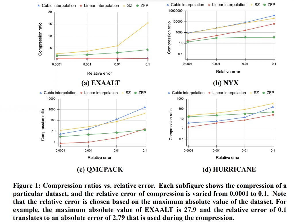
This work uses the absolute error for error control. The error can be calculated by multiplying the relative error (e.g, 10%) by the maximum absolute value of the data. This error metric is commonly known as relative L-infinity error in the literature. Figure 1 shows the relationship between compression ratio and relative error across four datasets, EXAALT, NYX, QMCPACK, and HURRICANE, respectively. The performances of linear and cubic interpolations are compared with state-of-the-art compressors SZ and ZFP. It is observed that the general trend is that as the relative error is loosened from 0.0001 to 0.1, the compression ratio improves substantially. This is because, as the relative error increases, the interval of a quantization bucket becomes larger, and therefore more data points can be grouped into a bucket during quantization, thus resulting in more repeated buckets and, in turn, higher compressibility of data. More importantly, it is shown in Figure 1 that the cubic interpolation outperforms the linear interpolation significantly across all datasets.  For example, the QMCPACK dataset undergoing cubic interpolation has an average compression ratio of 425.2, which is two orders of magnitude higher than that of the linear interpolation, which has an average compression ratio of 5.0. The reason for higher compression ratios for cubic interpolation is that it can better predict the data values, and therefore, it is more likely to achieve repeated values after quantization. Under tight error bounds (<0.1), the EXAALT dataset’s linear interpolation achieves similar compression ratios as cubic. The reason is that the EXAALT data varies significantly and is hard to compress. As a result, the cubic interpolation still suffers from inaccurate prediction. On the other hand, it is observed that the cubic can outperform SZ and ZFP for NYX and QMCPACK, demonstrating its performance advantage in certain scenarios as compared to the best compressors in the literature.

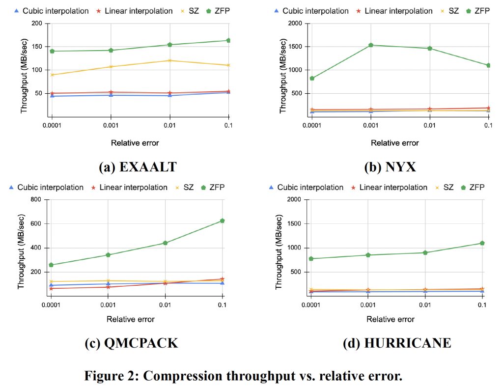
Figure 2 measures the throughput across various error bounds. The timing of compression was obtained by adding a pair of C/C++ clock() functions, which return the number of clock ticks elapsed since the test was launched. The clock() functions are inserted before and after the compression routine is invoked, respectively. The throughput is then calculated by dividing the size of the input data by the compression time.  In general, cubic interpolation requires more time to compress data due to the use of more data points for interpolation (discussed in Algorithm 6) and therefore, its throughput is expected to be lower than that of linear interpolation. An exception to this trend is the throughput for QMCPACK where under tight error bounds, the linear interpolation results in a lower throughput. This can be explained as follows.  The compression algorithms developed in this work mainly consist of two steps: interpolation and lossless encoding. Since linear involves fewer neighboring data points, its overhead is lower than that of cubic. However, the lossless encoding for linear interpolation is observed to have higher overhead than cubic because of the data characteristics of QMCPACK. For example, we collected the timings of compression for both linear and cubic interpolations for QMCPACK at an error of 0.0001. For cubic interpolation, the interpolation operation takes 5.7 secs and RLE takes 0.98 secs. For linear interpolation, the interpolation operation takes a shorter time of 3.67 secs, as expected, but RLE takes 5.37 secs, which is much longer than cubic. This caused the slower throughput of linear interpolation-based compression. Furthermore, it is observed that ZFP offers the highest compression throughput, while for certain scenarios, the linear interpolation can outperform SZ. Cubic, due to its high complexity, has the lowest throughput.

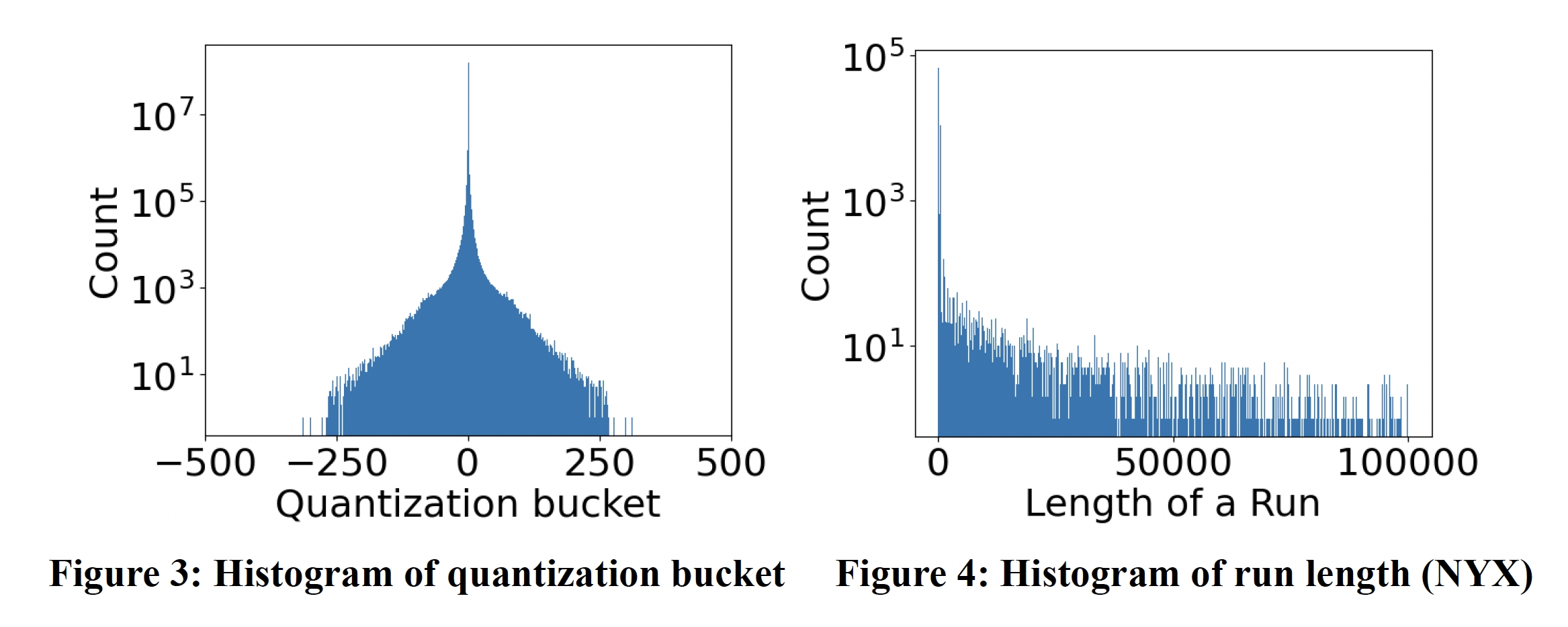
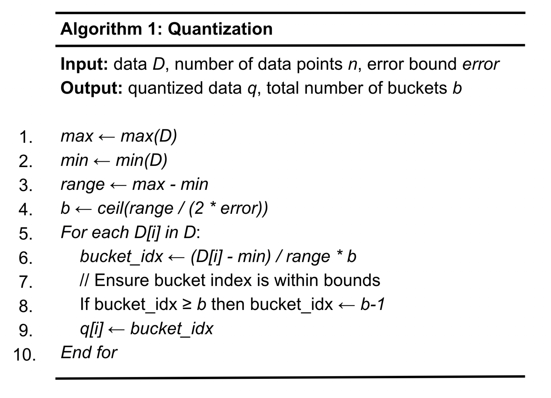
Figure 3 shows the histogram of quantization levels for NYX for cubic, where the X-axis is the bucket number and the Y-axis is the times a bucket is used to encode a data point. It is clear that the histogram follows a Gaussian distribution, which indicates that after cubic interpolation, the delta tends to center around zero, and the smaller the delta is, the higher the count is. Figure 4 further shows the histogram of run length for the NYX data. Clearly, the compression results in many long runs and leads to high compression ratios.

Tables 1 and 2 calculate the average compression ratios and throughputs, and can be used to further prove that cubic interpolation produces a higher compression ratio than that of linear interpolation, with the trade-off of lower throughput than linear interpolation, however. The reason for higher compression ratios for cubic interpolation is that it can better predict the data values, and therefore it is more likely to achieve repeated values after quantization. It is important to note that these trends depend on the input data characteristics and may not hold consistently for every single dataset. In general, for data that is relatively smooth, linear interpolation can be used to capture the trend of data while incurring less overhead as compared to cubic interpolation. For data that changes rapidly, cubic interpolation can be used to best capture the trend of the data in order to achieve a high compression ratio. Tables 3 and 4 further calculate the standard deviation of throughput for linear and cubic interpolation, respectively, across 5 consecutive runs. Overall, since there is no external interference on the system that was tested, the throughput variation is small.

Overall, the results contribute to the research field by comparing cubic to linear interpolation for a well-adopted lossless encoding scheme, and demonstrate its vastly improved compression ratios, which is fully expected by our hypothesis. A key limitation of this work is that it only uses RLE as the lossless compressor to demonstrate the effectiveness of high-order methods. Also, the throughput performance was conducted at a local computer, rather than a large-scale supercomputer, due to limited access to computing facilities. In the future, more effective lossless compression methods, such as the Huffman tree, will be implemented, which is expected to further improve the performance of cubic interpolation.

Methods

General Techniques

In this section, we will describe the compression algorithms implemented in this paper. The focus of this paper is to conduct algorithmic studies on interpolations, rather than on quantizations. Therefore, this work adopts the simple uniform quantization used in many lossy compressors, such as SZ. Algorithm 1 describes the basic uniform quantization technique that is used in both linear and cubic interpolation. This algorithm takes the input data D of n data points along with the prescribed error tolerance error, and produces the quantized data q. Note that this work performs 1D compression and it is expected that once the compression is done in higher dimensions (e.g., 3D), which were already explored by the existing tools, including SZ and ZFP,  will further improve the performance of both linear and cubic interpolations. In particular, from lines 1 to 2, we calculate the max and min of the input data so that we can determine the range of values for quantization in line 3. For uniform quantization, each quantization bucket has an equal size, and line 4 calculates the number of buckets by dividing the range of data by the size of a bucket (2*error). From lines 5 to 10, the algorithm iteratively quantizes each data point D[i], which is the value of the i-th data point. In particular, line 6 converts the value of D[i] to a bucket with its index being (D[i] – min) / range * b. Finally, in Line 9, the bucket index is stored in an array for quantized data q.Clearly, the time complexity of the algorithm of O(n).

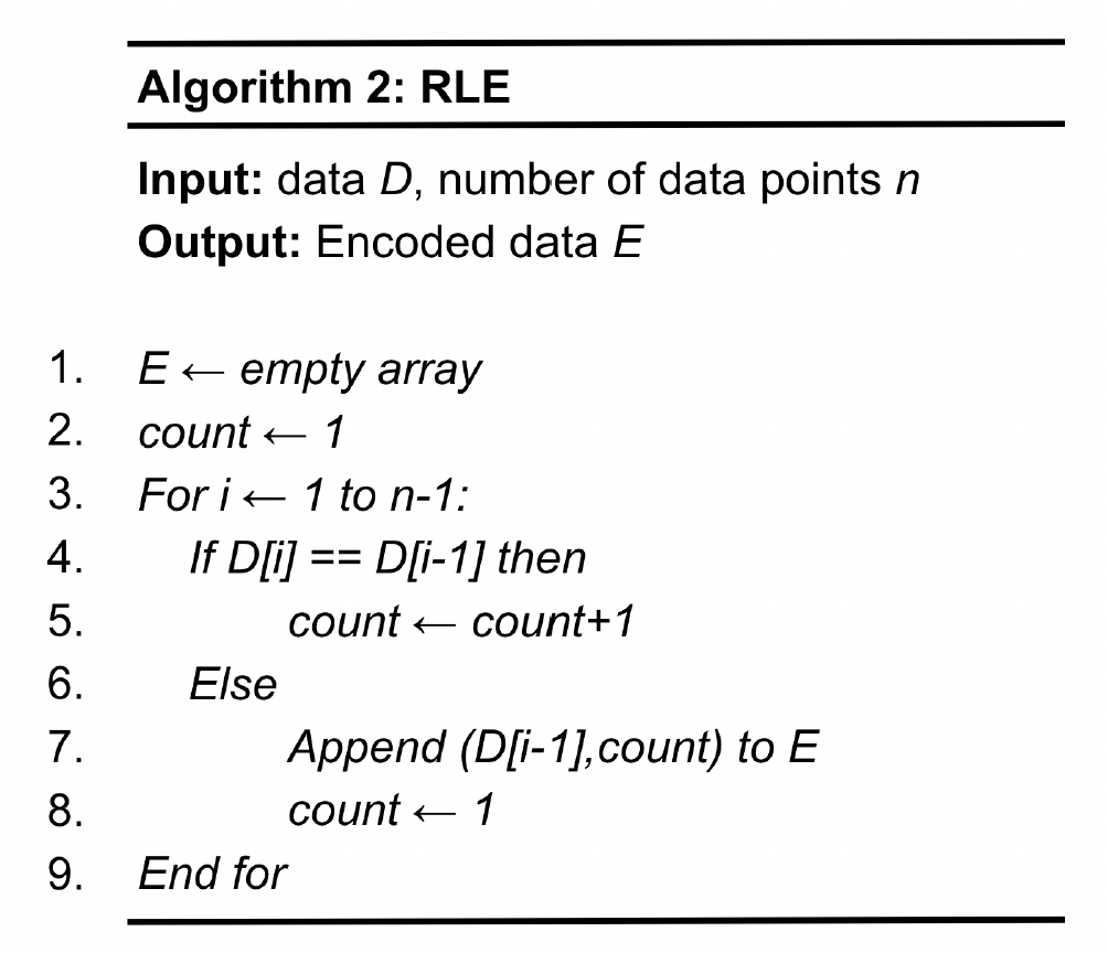
Once the data is quantized, it can then be compressed by RLE, as shown in Algorithm 2. RLE takes the quantized data D and produces the encoded data E. Line 1 allocates the memory space for the encoded data. Lines 3 to 9 go through the entire dataset, and if the two adjacent data points, D[i] and D[i-1], have the same value (Line 4), a counter (count), which records the times a data value appears in a consecutive manner, will be incremented by one (Line 5). This process will be repeated until a different value is encountered (Line 6), and the resulting run-length pair will be appended to the encoded data (Line 7) with the counter (count) reset to 1 to identify the next run (Line 8). Algorithm 3 shows the run-length decoding. In particular, Lines 4 to 6 convert a run-length pair to the original data by repeating a symbol for count times. The time complexity of RLE is O(n).

Linear interpolation with error control

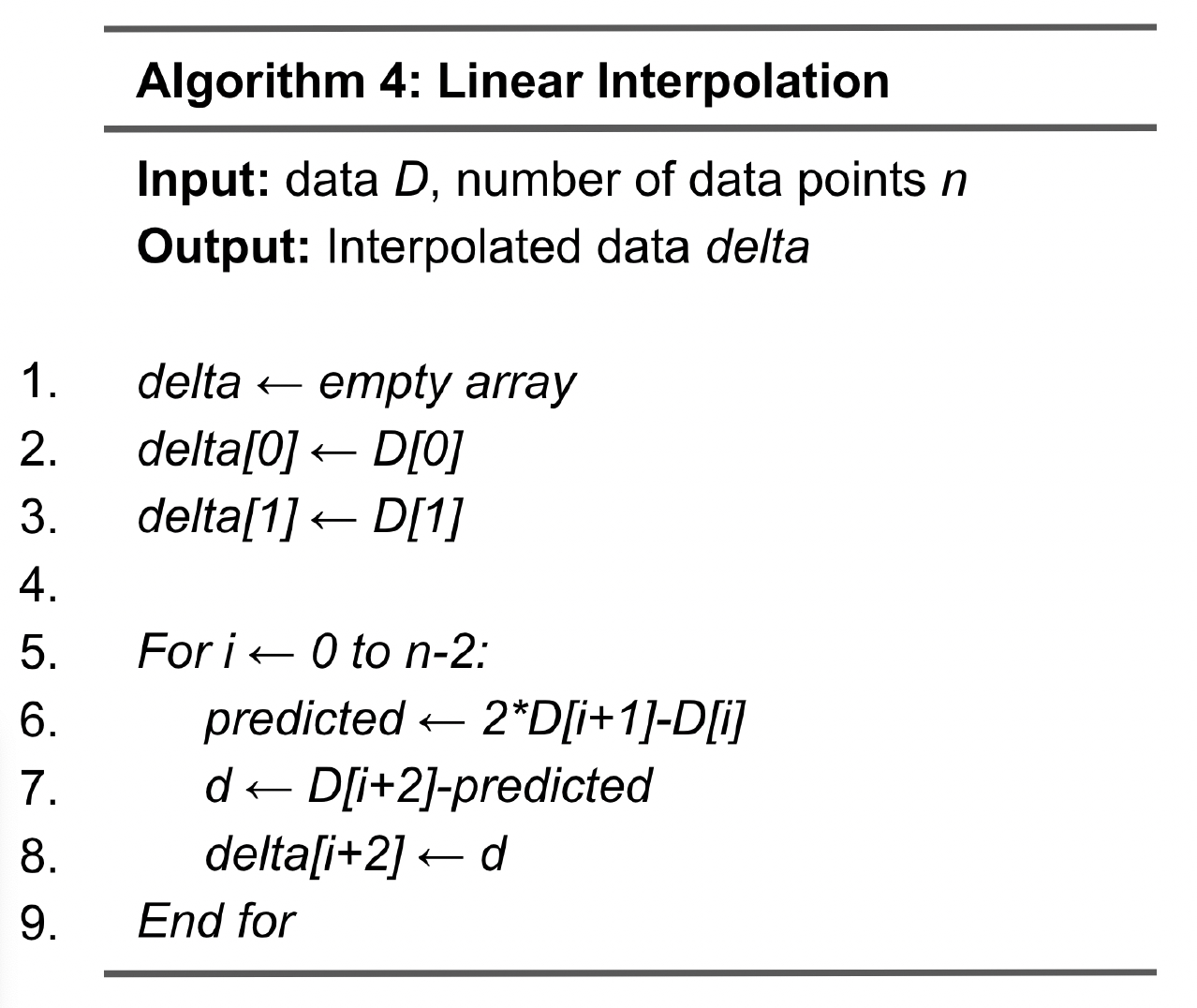
Algorithm 4 shows the steps to implement linear interpolation. From lines 1 to 3, variable delta is allocated memory space with delta[0] and delta[1] initialized to D[0] and D[1], respectively. Then, from lines 5 to 9, the algorithm loops through the rest of the data points and performs linear interpolation. At line 6, the predicted value (variable predicted) for data point i+2 is calculated by linearly extrapolating the values of D[i] and D[i+1]. We then compute the delta by subtracting the predicted value from the original value D[i+2] (Lines 7 and 8). The output of linear interpolation will be further quantized and compressed.

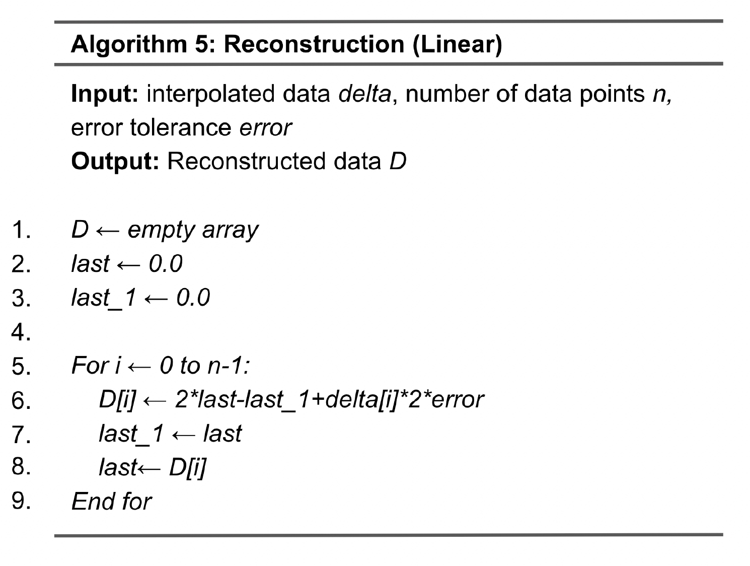
The data reconstruction for linear interpolation, as shown in Algorithm 5, is the inverse process of compression. The input to reconstruction is quantized data. Lines 5 to 9 loop through all data points where the variables last and last_1 capture the values of the two previous quantized data points, respectively. Line 6 calculates the predicted value by computing 2*last-last_1, and this will be added by the delta, which is delta[i]*2*error. Lines 7 and 8 update last_1 and last for calculating the next data point.

Cubic interpolation with error control

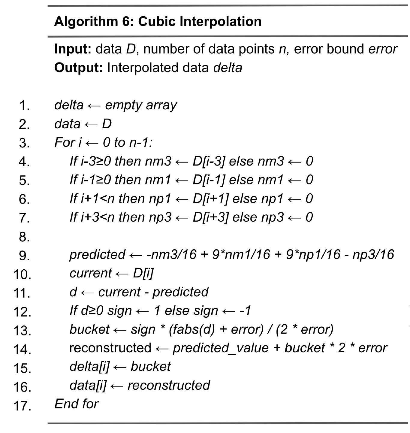
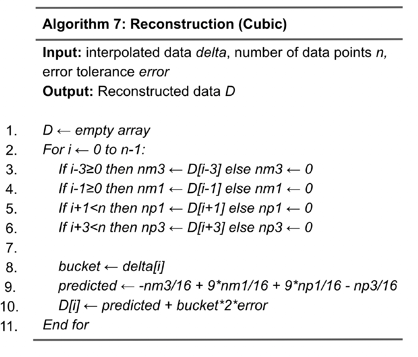
Algorithm 6 shows the steps of cubic interpolation. As compared to linear interpolation, which involves two adjacent data points, cubic interpolation uses four neighboring data points for a better quality of prediction. In particular, for data point D[i], it utilizes the values of D[i-3], D[i-1], D[i+1], and D[i+3], captured by variables nm3, nm1, np1, np3, respectively. The predicted value of D[i] is calculated in Line 9 as -nm3/16+9*nm1/16+9*np1/16-np3/16, and the delta d is calculated in line 11. Next, in lines 12 to 13, the delta is mapped to a bucket. Overall, the quantization is designed as follows: the range of bucket 0 is [-error, error] and the range of bucket 1 is [error, 3*error], and so on. Therefore, given delta d, the bucket assigned is sign*(fabs(d)+error)/(2*error), where fabs(d) is the absolute value of d and variable sign is the sign of d. Algorithm 7 shows the steps of reconstruction for cubic interpolation. As compared to the reconstruction for linear interpolation (Algorithm 5), the main difference is the calculation of the predicted value in line 9, which involves nm3, nm1, np1, and np3.

Both linear and cubic interpolations have a time complexity of O(n) since both algorithms involve going through all data points at once, and each iteration involves 2 and 4 neighboring data points for interpolation, respectively (see Algorithms 6 and 7). In terms of space complexity, for both algorithms, the memory consumption is O(n) for array allocation for variables delta (see lines 1 and 2 in Algorithm 6 for cubic interpolation) and variable D (see line 1 in Algorithm 7) for reconstruction.

Experimental setup

The experiment in this paper was conducted with an iMac with an Apple M3 processor, 16 GB of LPDDR5 memory, and 1 TB solid-state drive (SSD). The coding was done in Visual Studio Code 1.93.1 with GCC compiler (clang-1400.0.29.202). This work tested four real datasets, EXAALT, NYX, QMCPACK, and HURRICANE, provided by the Scientific Data Reduction Benchmarks⁷. They are described below.

• EXAALT: It is produced by a molecular dynamics simulation from Los Alamos National Laboratory. In particular, the field of zz.dat2 was used for the performance evaluation.  This dataset is 1D with 2,869,440 data points.
• NYX: It is produced by an adaptive mesh hydrodynamics + N-body cosmological simulation developed at Argonne National Laboratory. In particular, the field of baryon_density.f32 was used for the testing. This dataset is 3D with 512×512×512 data points. In this work, it is linearized into 1D for compression.
• QMCPACK: It is produced by a many-body ab initio Quantum Monte Carlo simulation. In particular, the field of einspline_288_115_69_69.f32 is compressed using the two interpolations. This dataset is 3D with 69×69×115 data points.
• HURRICANE: It is produced by a weather simulation. The field of CLOUDf48.bin.f32 is tested, which is a 3D dataset with 100×500×50 data points.

Conclusions and future work

This paper aims to develop and compare the two spline interpolations—linear and cubic interpolation—for scientific data reduction and evaluate their performance for run-length encoding. The results show that the cubic interpolation significantly improves the compression ratio as compared to the linear interpolation. In the future, adaptive interpolation schemes, where different interpolation schemes are used in different regions of data, will be developed to take advantage of the high compression ratios achieved by the cubic interpolation and the high throughput achieved by the linear interpolation. In addition, more advanced encoding schemes, such as Huffman, will be investigated.

References

1. Prabhat, Q. Koziol. High Performance Parallel I/O (1st ed.). Chapman and Hall/CRC. (2014). [↩]
2. J. Bennett et al. Combining in-situ and in-transit processing to enable extreme-scale scientific analysis. Proceedings of the International Conference on High Performance Computing, Networking, Storage and Analysis, Salt Lake City, UT, USA, 2012, pp. 1-9, doi: 10.1109/SC.2012.31. (2012). [↩]
3. T. Lu et al. Understanding and Modeling Lossy Compression Schemes on HPC Scientific Data. IEEE International Parallel and Distributed Processing Symposium (IPDPS), Vancouver, BC, Canada, 2018, pp. 348-357, doi: 10.1109/IPDPS.2018.00044. (2018). [↩]
4. X. Liang et al. Error-Controlled Lossy Compression Optimized for High Compression Ratios of Scientific Datasets. IEEE International Conference on Big Data (Big Data), Seattle, WA, USA, 2018, pp. 438-447, doi: 10.1109/BigData.2018.8622520. [↩]
5. P. Lindstrom. Fixed-Rate Compressed Floating-Point Arrays. IEEE Transactions on Visualization and Computer Graphics 20(12), 2674–2683 (2014). [↩]
6. Q. Gong et al. MGARD: A multigrid framework for high-performance, error-controlled data compression and refactoring, SoftwareX 24, (2023). [↩]
7. K. Zhao, S. Di, X. Liang, S. Li, D. Tao, J. Bessac, Z. Chen, and F. Cappello. SDRBench: Scientific Data Reduction Benchmark for Lossy Compressors. International Workshop on Big Data Reduction (IWBDR2020), in conjunction with IEEE Bigdata20. (2020). [↩]