Data-Driven Prediction of Tennis Ranking Movements with Ensemble Machine Learning Models

Abstract

Tennis rankings are central to evaluating player performance, determining tournament seedings, and influencing sponsorship opportunities. Traditional ranking systems like ATP and WTA often fail to capture players’ evolving dynamics and subtle performance shifts over time. This study introduces a machine learning-based framework with 9 models in total to predict player ranking movement using time series features derived from match statistics and historical performance data. A comprehensive dataset spanning ATP and WTA matches from 2013 to 2024 was compiled using web scraping methods, incorporating 31 features for the ATP dataset and 49 features for the WTA dataset, such as serve efficiency, return effectiveness, overall match statistics, and tournament-level results. Multiple regression models—including tree-based ensembles (e.g., LightGBM, XGBoost), linear models (e.g., Ridge, ElasticNet), and kernel methods (e.g., Kernel Ridge Regression)—were evaluated using MSE, RMSE, and MAE. A stacking ensemble with Kernel Ridge Regression as a meta-learner demonstrated the best predictive performance with the lowest error across all metrics. For the result, we also rank the feature importance for the LightGBM model to identify which match-level statistics contribute most significantly to ranking changes, providing data-informed training focuses, tactical planning, and performance analysis for coaches or players. The findings underscore the potential of ensemble machine learning approaches for accurate and data-driven player ranking forecasts in professional tennis.

Keywords: Tennis ranking, Time series, Machine learning, Data preprocessing, Modelling

Introduction

Tennis is one of the most popular racket sports in the world, with millions of recreational players and a huge population of spectators. In 2024, the combined viewership of the four Grand Slams, the major tennis tournaments, reached almost 2 billion people in more than 200 countries¹. Due to the competitiveness and global influence of tennis, the ranking of each player plays a central role in different areas. They determine tournament entries, seedings, and sponsorship deals while serving as a fundamental measurement of a player’s performance and ability. Thus, accurate and timely rankings of players are not only important for the players and coaches, but also for the stakeholders, sponsorships, and event organizers in the tennis community. Traditional ranking systems, such as the ATP and WTA point-based systems, only display raw numbers indicating a player’s performance in different categories and cannot fully capture the player’s evolving performance trends, especially when ranking is fluctuating all the time².

A possible solution is time series models, a technique that can perceive patterns in datasets to forecast future statistics. In the context of ranking in tennis, the primary features of determining whether a player is good or not are the player’s statistics and match outcomes in different level matches. By leveraging these key features, authorities can easily predict a player’s ranking movement, evaluating their potential commercially and tennis-wise. Many ML models have been developed for match outcome prediction because of the huge market for game betting³. However, an ML model and data set for tennis ranking prediction are relatively scarce due to the limited availability of comprehensive, high-quality player performance data over time. To address this issue and others, such as the scarcity of machine learning models focused on tennis ranking prediction, a data-driven approach that utilizes yearly player performance data is proposed. Our method begins by identifying the useful features and collecting data based on these features from the official ATP and WTA websites, or tennis datasets, like Ultimate Tennis Statistics, using BeautifulSoup for scraping⁴. Then, we preprocessed the data by normalizing the feature RankingMovement due to its large variability. At last, machine learning models that include ensemble models, tree-based models, and linear models are applied to predict the ranking movement of players⁵. By modelling player progression by data, our research aims to provide data-based insights to players, coaches, and tournament organizers.

While prior studies have explored predictive modeling in tennis, they have generally relied on limited datasets. They often restricted to single matches, shorter time periods, or specific tournaments. To our knowledge, no existing work has compiled a comprehensive dataset that spans both ATP and WTA players across more than a decade (2013–2024). This dataset contribution is therefore a novel aspect of our study. It enables broader and more representative modeling of ranking dynamics in male and female professional tennis.

Our main contributions are as follows:

1. We compile, to our knowledge, the first comprehensive dataset spanning both ATP and WTA players from 2013 to 2024, incorporating yearly player performance and match information from official and public sources.

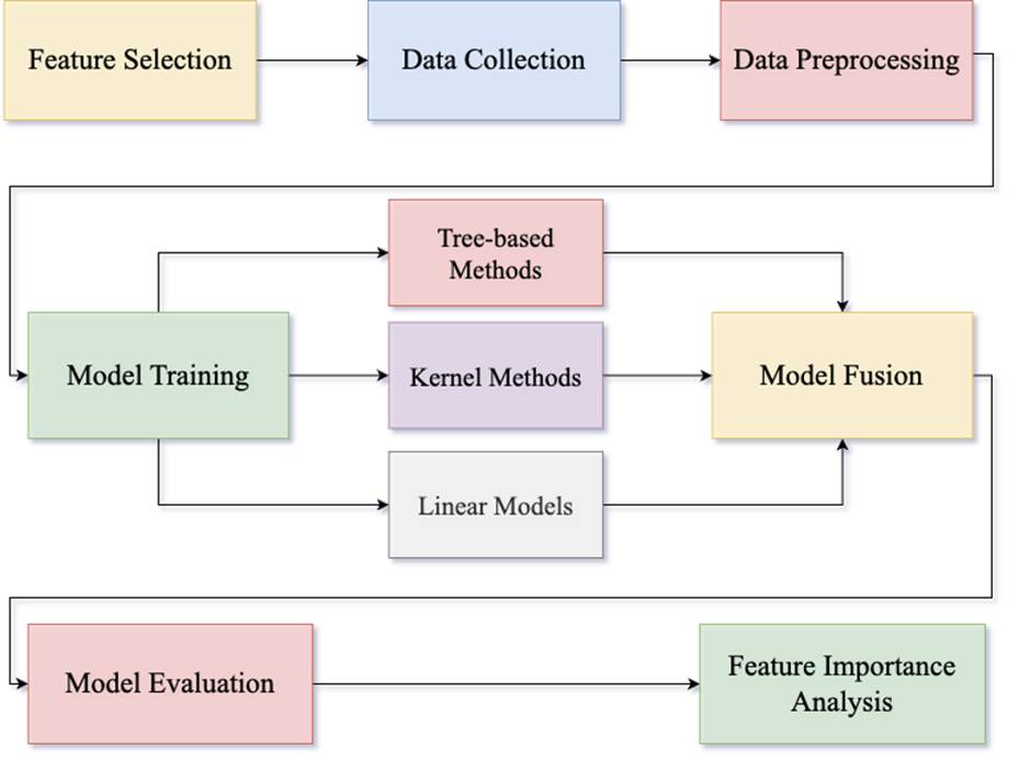
2. We design a machine learning pipeline with 9 models that leverages key player statistics to predict ranking movement, incorporating ensemble learning methods and model fusion for improved accuracy.

3. We provide empirical results and feature importance insights that can support players, coaches, and game organizers in understanding ranking dynamics and performance trends.

Literature Review

Player performance forecasting increasingly relies on machine learning modeling, integrating key factors, such as match statistics and historical rankings. Bozděch et al. introduced multinomial logistic regression and neural networks to identify key factors of ATP rankings, such as age, height, and service-related metrics⁶. Their study analyzed data from 1,990 tennis players during the 2022 season, with a total of 20,040 data points, highlighting the potential of neural networks in predicting ATP rankings.

Buhamra et al. uses various regression-based models, including random forests, spline-based approaches, and logistic regression to model and predict outcomes of men’s Grand Slam matches⁷. With a dataset of 5013 matches, the study considers diverse features, such as, ATP ranking and points, Elo rating, and betting odds. One notable thing this research introduced is the creation of two new variables, Age.30 and Age.int, which measure the deviation of age from 30 and an optimal interval. These features slightly improved the overall performance of the model. Bunker et al. compare the traditional Elo and WElo rating methods with machine learning models, including ANN, SVM, and Random Forest models, for predicting tennis match outcomes⁸. The study concludes that certain machine learning models, such as the Logistic Regression and ADTree models, outperformed the traditional rating method, matching the accuracy of betting odds. This underscores the potential of machine learning models in the field of tennis match outcome prediction, which is closely related to the prediction of player rankings.

Li introduced a logistic regression model grounded in Bayesian probability to predict point-level outcomes in a tennis match⁹. To consider the psychological factors in a match, the study employs the Analytic Hierarchy Process (AHP), with features, including rally length and first serve success rates, to quantify the momentum of a player. Pham et al. focus on the use of classification models, including XGboost, logistic regression, and random forest models, to forecast outcomes of ATP singles match¹⁰. The study utilizes a decade-long dataset ranging from 2012 to 2022, with up to 49 explanatory variables constructed of player statistics and match features. The random forest model in this study successfully predicted the winner, Novak Djokovic, of the 2023 Australian Open men’s singles tournament, demonstrating its accuracy. Lastly, Rui et al. introduced a supervised machine learning approach, using models such as, K-Nearest Neighbors, XGBoost, and logistic regression models, with XGBoost to predict the flow of points in a tennis match¹¹.The study utilizes Grey Relational Analysis and fuzzy set theory to rank several important features, including serve status, games won in the current set, ranking difference, distance covered, serve speed, previous victory status, and unforced errors. The study exhibited the potential of machine learning models when it comes to tennis-related forecasting.

Despite these advances, existing studies focus more on match outcome prediction rather than ranking dynamics, and often rely on datasets with limited time spans, or narrow feature sets. Few works incorporate both ATP and WTA players in a unified framework, while exploring the ranking dynamic of professional tennis in a comprehensive way.

Methods

Model Selection

This research evaluates the performance of several machine learning models, including LightGBM (LGB), XGBoost (XGB), Random Forest Regressor (RFR), Gradient Boosting Regressor (GBR), Extra Trees Regressor (ETR), Kernel Ridge Regression (KR), Ridge Regression (Ridge), ElasticNet (EN), and Bayesian Ridge Regression (BR). These models can be classified into five groups based on their underlying methodologies: Tree-Based Ensemble Methods (Random Forest Regressor, Extra Trees Regressor), Boosting Methods (LightGBM, XGBoost, Gradient Boosting Regressor), Bagging Methods (Random Forest Regressor, Extra Trees Regressor), Linear Models (Ridge Regression, ElasticNet, Bayesian Ridge Regression), and Kernel Methods (Kernel Ridge Regression). Tree-Based Ensemble Methods are machine learning models that aggregate the predictions of multiple decision trees to enhance performance and reduce overfitting. This research uses these diverse methods in a stacking framework, applying a 5-fold cross-validation repeated twice for better evaluation.

1. Tree-based ensemble methods are machine learning models that aggregate the predictions of multiple decision trees to enhance performance and reduce overfitting. The Random Forest Regressor fits a large number of decision trees on various subsets of data and averages their output to improve accuracy and control overfitting¹². In comparison, Extra Trees Regressor introduces more randomness by selecting splits randomly during tree construction, which may be better at avoiding overfitting¹³. These models capture non-linear relationships between player statistics, such as the interaction of first serve percentage and return game won percentage, which strongly influence ranking changes. Their averaging mechanisms reduce variance and make them robust to noise in yearly performance data.
2. Boosting methods sequentially refine predictions by correcting prior errors, which is particularly valuable for ranking prediction where small errors can accumulate into significant ranking shifts. Gradient Boosting Regressor builds a predictive model in the form of an ensemble of weak predictive models and optimizes a differentiable loss function over function space¹⁴. XGBoost improves gradient boosting with second-order derivatives (Hessian) and parallel computations for faster and more accurate optimizations¹⁵. Lastly, LightGBM uses a leaf-wise growth strategy rather than the classic level-wise methods and histogram-based techniques for a lower memory usage, offering greater efficiency for large datasets¹⁶.
3. Bagging methods focus on training multiple base models independently on different random subsets of the original dataset. Random Forest and Extra Trees are notable examples that apply bootstrapping (sampling with replacement) to create various models whose outputs are averaged to improve generalization and reduce overfitting¹⁷.
4. Linear models offer interpretability and serve as strong baselines for understanding how individual features, such as aces or break points converted, contribute to ranking changes. Ridge regression is a linear regression model that uses L2 regularization to shrink coefficients and reduce overfitting¹⁸. ElasticNet is a linear model that incorporates both L1 (lasso) and L2 (ridge) regularization, which offers both coefficient shrinkage and feature selection¹⁸. Lastly, Bayesian Ridge Regression is a type of conditional modeling in which coefficients are treated as random variables, with the goal of estimating their distributions to capture uncertainty in predictions¹⁸.
5. Kernel methods are a class of algorithms of pattern analysis, which utilizes kernal function to map input data into higher-dimensional spaces, allowing the linear models to capture non-linear relationships. Kernel Ridge Regression combines Ridge regression (linear model) with kernel methods, which gives the model more flexibility when fitting and less overfitting with the help of the L2 penalty¹⁸.

Dataset and Splits

The dataset includes ATP and WTA player yearly performance data from 2013 to 2024, sourced from the official ATP and WTA Tour website and Ultimate Tennis Statistics, which is an online ATP database made by Cekovic¹⁹. The ATP dataset includes up to 31 explanatory variables, ranging from match statistics such as first serve percentage and aces to historical features like match records and player rankings.

Serve performance, return performance, overall match performance, historical match records, and ranking information are the most substantial features in determining a player’s overall performance. Thus, it is important to capitalize on these features when training an ML model to predict the ranking of players.

Precise ranking predictions deeply rely on the consideration of the quality and effectiveness of player’s serve. Key variables include Aces, DoubleFaults, 1stServe percentage, and points won on both first and second serves. Additional features such as BreakPointsFaced, BreakPointsSaved, ServiceGamesPlayed, ServiceGamesWon, and TotalServicePointsWon provide an overall view of a player’s serve consistency and ability to maintain service under pressure. All of the above features either reflect the direct effectiveness of serve, such as the number of aces, which is a successful serve that the opposing player does not touch, or indirectly reflect the effectiveness of a serve, for example, service games won.

Similar to the serve, the return also plays a crucial role in a tennis match. It determines how effectively a player can handle pressure from the opponent’s serve and service games, which indirectly indicates the opportunity a player has to break the opponent’s serve. Variables such as 1stServeReturnPointsWon, 2ndServeReturnPointsWon, BreakPointsOpportunities, and BreakPointsConverted measure return efficiency and conversion rates. More directly, ReturnGamesPlayed, ReturnGamesWon, and ReturnPointsWon give insight into return dominance and consistency.

Certain players may have a high percentage in the above features due to the lower-level tournament they have participated in. Thus, it is important to consider the level of matches they are playing in and how they are performing. These include counts of matches won and lost in Grand Slams, Masters 1000, ATP 500, and ATP 250 events. This also indirectly reflects how a player handles pressure and different levels of opponents.

Lastly, since we are predicting the ranking of players, it is crucial to include their ranking in the previous year and the ranking movement. This is the most direct reflection of how the player has performed in the entire year.

The dataset is then separated into a training dataset and a test dataset with a ratio of 4:1.

Feature Name	Description
PlayerID	Unique identifier for each player.
Aces	Number of service aces made by the player.
DoubleFaults	Number of double faults committed by the player.
1stServe	Percentage of first serves successfully made.
1stServePointsWon	Percentage of points won on first serve.
2ndServePointsWon	Percentage of points won on second serve.
BreakPointsFaced	Total number of break points faced on serve.
BreakPointsSaved	Number of break points saved on serve.
ServiceGamesPlayed	Total number of service games played.
ServiceGamesWon	Number of service games won.
TotalServicePointsWon	Total percentage of service points won.
1stServeReturnPointsWon	Percentage of opponent’s first serve points won by the player.
2ndServeReturnPointsWon	Percentage of opponent’s second serve points won by the player.
BreakPointsOpportunities	Total number of break points opportunities the player had against opponents.
BreakPointsConverted	Number of break points successfully converted against opponents.
ReturnGamesPlayed	Number of return games played.
ReturnGamesWon	Number of return games won.
ReturnPointsWon	Percentage of points won while returning serve.
TotalPointsWon	Percentage of total points won (serve + return).
GrandSlamWon	Number of Grand Slam matches won.
GrandSlamLost	Number of Grand Slam matches lost.
MastersWon	Number of ATP Masters 1000 matches won.
MastersLost	Number of ATP Masters 1000 matches lost.
ATP500Won	Number of ATP 500 matches won.
ATP500Lost	Number of ATP 500 matches lost.
ATP250Won	Number of ATP 250 matches won.
ATP250Lost	Number of ATP 250 matches lost.
CurRanking	Current ATP ranking.
PrevRanking	Previous ATP ranking.
RankingMovement	Change in ATP ranking compared to the previous ranking (CurRanking – PrevRanking).

Feature Name	Description
PlayerNbr	Unique identifier for each player.
Aces	Number of service aces made by the player.
DoubleFaults	Number of double faults committed by the player.
FirstServesWon	Number of points won on first serve.
FirstServesPlayed	Total number of first serves attempted.
SecondServesWon	Number of points won on second serve.
SecondServesPlayed	Total number of second serves attempted.
BreakPointsFaced	Total number of break points faced on serve.
BreakPointsLost	Number of break points lost on serve.
ServiceGamesPlayed	Total number of service games played.
ReturnGamesPlayed	Total number of return games played.
BreakPointChances	Total number of break point opportunities against opponents.
BreakPointsConverted	Number of break points successfully converted.
FirstServeReturnChances	Number of opponent’s first serves returned.
FirstReturnWon	Number of points won on opponent’s first serve.
SecondReturnChances	Number of opponent’s second serves returned.
SecondReturnWon	Number of points won on opponent’s second serve.
FirstServeWonPercent	Percentage of points won on first serve.
SecondServeWonPercent	Percentage of points won on second serve.
FirstReturnPercent	Percentage of points won on opponent’s first serve.
SecondReturnPercent	Percentage of points won on opponent’s second serve.
BreakpointConvertedPercent	Percentage of break points converted.
FirstServePercent	Percentage of first serves successfully made.
ReturnGamesWonPercent	Percentage of return games won.
BreakpointSavedPercent	Percentage of break points saved.
ServiceGamesWonPercent	Percentage of service games won.
ServicePointsWonPercent	Percentage of total service points won.
ReturnPointsWonPercent	Percentage of total return points won.
TotalPointsWonPercent	Percentage of all points won (serve + return).
MatchCount	Number of matches played.
AcesPerMatch	Average number of aces per match.
DoubleFaultsPerMatch	Average number of double faults per match.
FirstServesWonPerMatch	Average number of first serve points won per match.
FirstServesPlayedPerMatch	Average number of first serves attempted per match.
SecondServesWonPerMatch	Average number of second serve points won per match.
SecondServesPlayedPerMatch	Average number of second serves attempted per match.
BreakPointsFacedPerMatch	Average number of break points faced per match.
BreakPointsLostPerMatch	Average number of break points lost per match.
ServiceGamesPlayedPerMatch	Average number of service games played per match.
ReturnGamesPlayedPerMatch	Average number of return games played per match.
BreakPointChancesPerMatch	Average number of break point opportunities per match.
BreakPointsConvertedPerMatch	Average number of break points converted per match.
FirstServeReturnChancesPerMatch	Average number of opponent’s first serves returned per match.
FirstReturnWonPerMatch	Average number of first serve return points won per match.
SecondReturnChancesPerMatch	Average number of opponent’s second serves returned per match.
SecondReturnWonPerMatch	Average number of second serve return points won per match.
CurSinglesRanking	Current ATP singles ranking.
PrevSinglesRanking	Previous ATP singles ranking.
RankingMovement	Change in ATP singles ranking (CurSinglesRanking – PrevSinglesRanking).

Data Preprocessing

Due to the larger variation of the feature Rankingmovement in the WTA dataset, every value in the feature Rankingmovement is scaled in the range of [-80,80], meaning that any value that is greater than 80 will be scaled down to 80, and vice versa.

The data points of the feature ranking movement is standardized according to the formula:

where x is the original data point, is the minimum value in the dataset, and  is the maximum value in the dataset. This standardization scales all the data in [0,1] and ensures that the feature contributes appropriately to model training without being impacted by the scale of other variables, especially when the ranking movement has a wide range of values, with a maximum absolute value of up to 100²⁰.

Hyperparameter Tuning

To optimize model performance, we applied Exhaustive Grid Search for each model. This method systematically explores all possible combinations within the generated grid to identify the optimal configuration that yields the best cross-validation performance.

Each combination is evaluated using 5 fold-cross validation, and the optimal set of parameters was selected based on the lowest validation MSE. This exhaustive grid search allowed the model to perform at its best.

Fusion Model

In this pipeline, each of the nine base models (tree-based ensembles, boosting methods, linear regressors, and kernel methods) was first trained on the training dataset using 5-fold cross-validation repeated twice. For each fold, the base models generated out-of-fold predictions that were not used during their own training. These predictions were then fused to form a collective output of the base models.

The choice of KRR as the meta-learner is motivated by its ability to capture nonlinear interactions among the base model outputs. KRR also applies L2 regularization to prevent overfitting. Unlike other meta-learners, KRR emphasizes stronger base learners in the pipeline while diminishing the influence of weaker ones. A fusion model efficiently combines the advantages of different models, producing a superior result.

Results

Model	MSE	RMSE	MAE
LightGBM	0.04437981	0.2106651609	0.16518502
XGboost	0.04612287	0.214762357	0.16784685
RandomForestRegressor	0.04370014	0.2090457845	0.16392416
GradientBoostingRegressor	0.04369567	0.2090350927	0.16420869
ExtraTreesRegressor	0.04399656	0.2097535697	0.16459271
Kernel Ridge Regression	0.04409751	0.2099940713	0.16623350
Ridge Regression	0.04388663	0.2094913602	0.16590699
ElasticNet	0.04688098	0.2165201607	0.17132136
BayesianRidge	0.04394150	0.2096222794	0.16598605
Fusion	0.04326192	0.20799499	0.16317526

Model	MSE	RMSE	MAE
LightGBM	0.11385351	0.33742186	0.28567814
XGboost	0.11825046	0.34387565	0.28579842
RandomForestRegressor	0.11436906	0.33818495	0.28429549
GradientBoostingRegressor	0.11405787	0.33772455	0.28461343
ExtraTreesRegressor	0.11376552	0.33729145	0.28456482
Kernel Ridge Regression	0.11550158	0.33985523	0.28443830
Ridge Regression	0.11527410	0.33952040	0.28530757
ElasticNet	0.11472408	0.33870943	0.28602896
BayesianRidge	0.11456985	0.33848168	0.28565093
Fusion	0.11406168	0.33773019	0.28453259

We take Mean Squared Error (MSE), Root Mean Squared Error (RMSE), and Mean Absolute Error (MAE) into account when analyzing the performance of the different models.

MSE is a cost function that measures the average of the squares of the errors. The function emphasizes larger errors, which may be helpful for certain data, like financial forecasting, where large errors are more detrimental. However, it may perform worse with the occurrence of outliers, so it could be better to consider the MAE. MAE measures the average magnitude of the errors in a set of predictions, without considering their direction. Similar to MSE, RMSE is a cost function that can be represented as the square root of the mean square error. Looking at the square root of MSE can be advantageous because of the similar scaling of RMSE and the data, and the lesser sensitivity towards outliers.

The models trained on the ATP dataset performed significantly better compared to the models trained on the WTA dataset across all metrics (MSE, RMSE, and MAE). The largest MAE increase between WTA and ATP models scales up to +0.1205 and +0.1204 in LightGBM and Random Forest Regressor. This indicates that the WTA dataset is much noisier and more heterogeneous compared to the ATP dataset, meaning it has a less predictive structure. In reality, in the feature RankingMovement, there is a much wider range, with an absolute value of up to 400, in the WTA dataset as in other features compared to the ATP dataset. The large difference in errors may suggest that male players have a more consistent performance and fewer performance swings when compared to female players, as well as less variability in overall outcomes.

Due to the diversity of models used in the process, accompanied by the differences, a fusion model, which combines the predictions of individual base models using Kernel Ridge Regression (KRR), is added. In both the ATP and WTA based models, the fusion model is seen to have the best performance over all metrics. This is likely because KRR captures nonlinear relationships between the base model outputs and the true target. This allows it to learn how to optimally weight and adjust their contributions, leading to better generalization on both ATP and WTA datasets. Moreover, the gap of +0.0708 between ATP and WTA models further suggests that the ATP dataset is more predictive.

Among the models tested from both the ATP and WTA datasets, tree-based models and ensemble methods such as LightGBM, Random Forest, and Gradient Boosting are observed to have a better overall performance compared to other linear models. Across the linear models, Elastic Net performs the worst, which may be due to the lesser flexibility of the model. This suggests that the relationship between ranking outcomes and the features used to measure player’s performance have a nonlinear relationship and involves complex interactions, which is better captured by tree-based models and ensemble methods. In comparison, linear models are more limited in modelling such patterns despite being more interpretable.

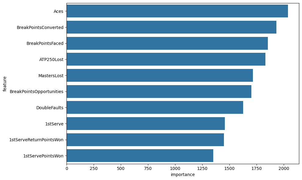
For the explanation about the models, we use LightGBM for feature important ranking, as shown in Fig. 3. For the ATP player, serves plays a crucial role in a tennis match, and a player with a successful serve can win large percentages of their service games. One great example is John Isner, who has a career-highest ranking at number 8 and had 1260 aces in 2015²¹. Aces are a great indicator of players’ serving performance, and a great serve reduces pressure while saving more games. It is evident that most of the top players have a strong and accurate serve. This suggests that coaches should prioritize training sessions focused on serve consistency and accuracy under pressure, as improvements here are most likely to translate into ranking gains.

The second important feature, BreakPointsConverted, measure how effectively a player deals with the service games of their opponent, their ability to handle critical points, and most of all, how effectively a player turns break point opportunities into actual breaks which, in many cases, a single break wins the player an entire round. On the opposite, the third important feature, BreakPointssaved, indicates dominance on serve, which is a common trait for high-ranking players.

The next two traits are direct measurements of a player’s performance in large tournaments—ATP 250 and Masters (ATP 1000). Frequent early losses in lower-tier (ATP 250) or high-tier (Masters) events can prevent ranking progression. It is reasonable for the model to rank ATP250 before the Masters tournament despite that the Masters being more prosperous and competitive than the ATP250 tournament, because only the top 50 players are the major participants in Masters events, while we took the top 300 players for both the ATP and WTA datasets.

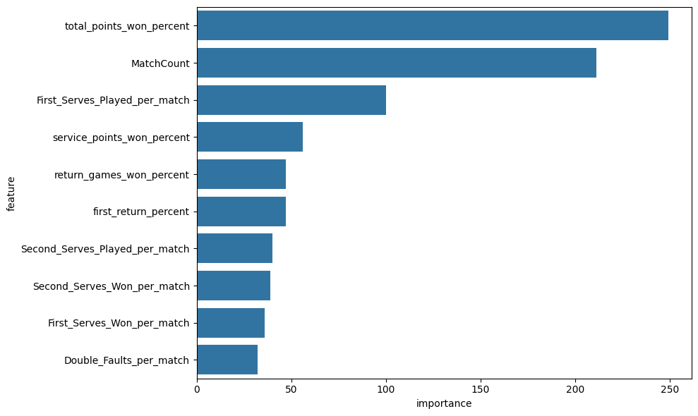
For the WTA players, Total_Points_Won_Percent plays the most important role in determining ranking movement. This is reasonable because the higher the percentage a player wins in total, the more dominance a player is showing in a match. The second most important feature, MatchCount, measures the number of matches a player has participated in in a year. A greater value for MatchCount indicates better performance stability and a higher ranking in general for those who progress more across all tournaments. This may also be caused by the nature of LightGBM, which often favors numerical figures with a broader range. However, based on the model’s ranking, players should prioritize playing more matches in different level to gain more experience.

After the two more dominant features in the WTA dataset, the third-ranked figure is rather similar to the ATP feature ranking, showing a feature related to serving. The number of first serves played per match directly indicates the percentage a player has to hold a serve or serve an ace. It can be a deciding factor in winning games. The fourth-ranked feature, ServicePointsWonPercent, quantifies a player’s overall effectiveness when serving by calculating the percentage of total service points won. Unlike features like aces or first serves won, this feature captures the complete view across all situations. A high value in this feature typically reflects strong serving consistency and the ability to hold serves. Both the third and fourth features indicate that serves play a crucial role in WTA tennis. The fifth feature, Return_Games_Won_percent, measures the ability of a player to break serves of the opponent, and in many cases, the player with a single break in a set takes the set.

Overall, most of the feature’s rankings are very reasonable and explainable based on tennis knowledge, which indicates that the model is making decisions based on meaningful and interpretable signals, not noise.

Conclusion

This study demonstrates the feasibility and effectiveness of using machine learning models to predict tennis player ranking movements based on match statistics and historical performance data. Unlike the ATP/WTA point systems, which only reflect past results and provide static standings, our framework offers forward-looking insights into ranking movements. By applying and comparing a diverse set of models—ranging from boosting techniques to linear regressions—we found that tree-based ensemble methods consistently outperform others, reflecting the nonlinear and complex nature of performance factors in tennis. Furthermore, the fusion model using kernel ridge regression yielded the most accurate predictions by capturing nonlinear relationships across model outputs. The performance gap between ATP and WTA datasets reveals a more stable and predictable structure in men’s tennis rankings, highlighting differences in performance variance and data quality. These insights have practical implications for stakeholders across the tennis ecosystem, from analysts and coaches to media and sponsors. Future work could expand to include real-time data, psychological metrics, and player health indicators to further enhance model robustness and predictive accuracy. These enhancements would allow the model to generate more precise, context-aware ranking forecasts, while including certain aspects that is difficult to incorporate for our current model. Beyond methodological gains, such predictions can more comprehensively support players and coaches in training focus, tournament scheduling, and workload management.

References

1. Roland-Garros. Worldwide audiences for Grand Slam tennis reach new records. https://www.rolandgarros.com/en-us/article/worldwide-audiences-grand-slam-tennis-record-onsite-tv-social-media (2024). [↩]
2. Universal Tennis Rating. Global tennis player rating system. https://en.wikipedia.org/wiki/Universal_Tennis_Rating (2025). [↩]
3. I. McHale, A. Morton. A Bradley-Terry type model for forecasting tennis match results. Journal of Mathematical Psychology (2011). [↩]
4. A. Kamra. Predicting ATP Player Tennis Performance Using Machine Learning. Statistics were compiled from Ultimate Tennis Statistics and ATP Tour databases. [↩]
5. M. Bozděch, D. Puda, P. Grasgruber. A detailed analysis of game statistics of professional tennis players: An inferential and machine learning approach. PLoS ONE 19(11) (2024). [↩]
6. M. Bozděch, D. Puda, P. Grasgruber. A detailed analysis of game statistics of professional tennis players: An inferential and machine learning approach. PLoS ONE. 19(11), e0309085 (2024). [↩]
7. N. Buhamra, A. Groll, S. Brunner. Modeling and prediction of tennis matches at Grand Slam tournaments. J Sports Analytics. 10(1), 17–33 (2024). [↩]
8. R. Bunker, C. Yeung, T. Susnjak, C. Espie, K. Fujii. A comparative evaluation of Elo ratings- and machine learning-based methods for tennis match result prediction. Journal of Sports Analytics.(2024). [↩]
9. C. Li, Research on dynamic analysis and prediction model of tennis match based on Bayesian probability and analytic hierarchy process. arXiv preprint arXiv:2407.07116 (2024). [↩]
10. C. Pham, K. Bufi. Predicting tennis match results using classification methods. Master’s Essay, Department of Economics, Lund University. (2023). [↩]
11. B. Rui, C. Kar Hing, L. Haoyuan, T. Jia Yew. Forecasting Tennis Player Matches Based on Machine Learning. Proceedings of 2024 International Conference on Machine Learning and Intelligent Computing, PMLR 245, 393–403 (2024). [↩]
12. J. Han, M. Kamber, J. Pei. Data Mining: Concepts and Techniques. 3rd ed., Morgan Kaufmann, 2011. [↩]
13. T. Hastie, R. Tibshirani, J. Friedman. The Elements of Statistical Learning: Data Mining, Inference, and Prediction. 2nd ed., Springer, 2009. [↩]
14. C. Bishop. Pattern Recognition and Machine Learning. Springer, 2006. [↩]
15. T. Chen, C. Guestrin. XGBoost: A Scalable Tree Boosting System. Proceedings of the 22nd ACM SIGKDD International Conference on Knowledge Discovery and Data Mining, 785–794 (2016). [↩]
16. G. Ke et al. LightGBM: A Highly Efficient Gradient Boosting Decision Tree. Advances in Neural Information Processing Systems 30 (NeurIPS 2017), 3146–3154 (2017). [↩]
17. L. Breiman. Bagging predictors. Machine Learning 24(2): 123–140 (1996). [↩]
18. F. Pedregosa et al. Scikit-learn: Machine Learning in Python. Journal of Machine Learning Research 12: 2825–2830 (2011). [↩] [↩] [↩] [↩]
19. Ultimate Tennis Statistics. Ultimate men’s tennis statistics destination for die-hard fans. https://www.ultimatetennisstatistics.com (2025). [↩]
20. Lucas B. V. de Amorim, George D. C. Cavalcanti & Rafael M. O. Cruz. “The choice of scaling technique matters for classification performance.” Patterns 3 (2022): 100401. [↩]
21. John Isner – Player stats. https://www.atptour.com/en/players/john-isner/i186/player-stats?year=2015&surface=all (2015). [↩]