Comparative Analysis of the Effectiveness of Deep Reinforcement Learning Models for Trading in the Stock Market

Abstract

Trading in the stock market presents many challenges to both individual and institutional traders. It demands a significant amount of time, knowledge, and risk tolerance. Even modern solutions such as algorithmic trading are purely statistical and don’t account well for market anomalies. Reinforcement learning, a branch of machine learning, is a potential technique used in designing algorithms for stock market trading. In this study, we compared the performance of 3 deep reinforcement learning algorithms to trade profitably in the stock market. The models were trained using Google’s historical stock prices exported from DI-Engine’s trading environment. To compare the models, we used 6 financial metrics that are provided by the QuantStats Python library: Cumulative Returns, Sharpe Ratio, Calmar Ratio, Sortino Ratio, Profit Factor, and Omega. Based on the results, the PPO model provided the highest cumulative returns of 62% when compared to the DQN model which gave 33%, and the A2C model which gave 45%. While the PPO model achieved the highest cumulative return, the A2C model had superior risk-adjusted performance with a Sharpe ratio of 2.11 and Sortino ratio of 5.47 – outperforming both PPO (Sharpe: 1.24, Sortino: 3.33) and DQN (Sharpe: 1.82, Sortino: 3.02) in balancing returns with volatility and downside risk. This made us conclude that the A2C model is more dependable than the PPO and DQN models. We hope that this paper will function as a foundation for future research which may involve the utilization of other data points including technical indicators, sentiment analysis as well as quarterly/annual results.

Keywords: Deep Reinforcement Learning, Stock Trading, Algorithmic Trading, Machine Learning

Introduction

The goal of investing in the stock market is not just to make money, but rather to generate profits consistently or at the very least beat the average yearly expected return (11%). For most hedge funds and investment firms, the goal is to consistently outperform the market itself, not just the average yearly expected return. For the average investor, however, the goal is more likely to outperform the 11% expected return. Unfortunately, the methods of doing so are not only enigmatic but are also inconsistent. For example, a research paper on the profitability of technical analysis shows that many studies are subject to various problems in their methodology, leading to mixed results¹. Quantitative trading algorithms are also not consistent in generating profits because many such algorithms are often overfitted to a specific time period of a certain stock and so they cannot predict market anomalies which are quite frequent in a dynamic, ever-changing market².

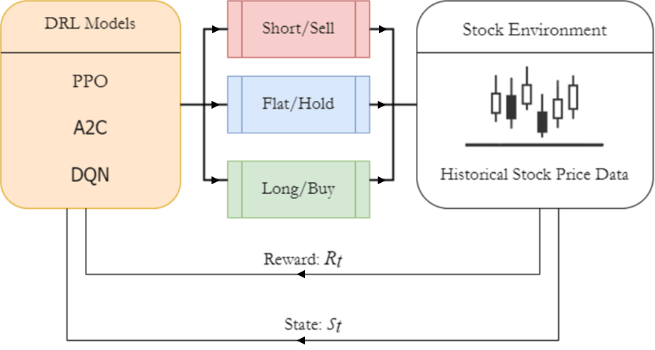
Deep reinforcement learning (DRL) may be able to bypass many of these issues while generating consistent returns. DRL combines deep neural networks with the “reinforcement learning” style³. This allows models to make live decisions and learn based on those decisions – similar to how a human trader would. However, the DRL models would be able to process more complex data within seconds and make instant decisions based on it. DRL models also bypass two fundamental issues with human traders: DRL models are less susceptible to emotional bias and can quickly adapt to changing markets⁴. Furthermore, because DRL models are trained using historical data, they will likely be able to deal with new market situations (bull market vs bear market) which some human traders may not have experienced entirely⁵. DRL models may also have the advantage compared to non-policy-based algorithms such as regressions or LSTM models because DRL models can detect market changes in general trends and market sentiment in real-time⁶.

We believe that this research is important as it has immense potential in providing access to complex trading tools for retail investors. We also feel that this research can help advance the field of algorithmic trading by opening future research towards different AI solutions for financial markets. In this paper, we hypothesize that among these three models of DRL, the PPO model will outperform the other 2 models by generating a greater cumulative return and by having better performance metrics. A detailed description of the experimental setup and model architecture is provided in the Materials and Methods section.

Literature Review

Machine Learning & Deep Learning Models in Stock Trading

Machine learning and deep learning techniques have been increasingly applied to stock market trading, though notable limitations are present. Supervised learning methods like Support Vector Machines (SVM) achieve hit ratios up to 60.07% in trend prediction but show poor adaptability to non-linear market dynamics⁷. Random Forest classification models have achieved prediction accuracies higher than 50% for stock price direction prediction. While Random Forest classifiers generate returns that exceed passive strategies, they struggle with temporal dependencies inherent in financial time-series data⁸. 

Deep learning techniques have emerged as more sophisticated alternatives. The Long Short-Term Memory (LSTM) model has shown potential for financial time-series prediction due to the nature of RNN’s ability to handle sequential data and incorporate historical information. LSTM ensembles have demonstrated better average daily returns, higher cumulative returns, and lower volatility compared to traditional portfolio approaches⁹. While these networks capture sequential patterns with 92.46% accuracy in controlled settings, they are prone to overfitting and fail during structural breaks. Convolutional Neural Networks (CNNs) have also been used to make financial predictions. CNNs convert time series data into image representations in combination with technical indicators to capture patterns in stock price movements. Studies have shown that CNN-based models can achieve up to 94.9% accuracy in predicting multiple stock market trend patterns¹⁰. Despite these advancements, traditional machine learning algorithms and deep learning models suffer from overfitting to specific time periods, thus impeding their ability to predict market anomalies in dynamic markets¹¹.

Deep Reinforcement Learning Models in Stock Trading

Deep reinforcement learning (DRL) addresses many of these fundamental limitations while generating consistent returns. Unlike supervised learning approaches that rely on historical labeled data and treat predictions independently, DRL combines deep neural networks with reinforcement learning principles, enabling models to learn optimal trading strategies through direct interaction with market environments. DRL models also eliminate the need for labeled training data as the models learn through trial-and-error interactions with the market¹². DRL models can adapt to dynamic market conditions through live learning, addressing the overfitting issue. Finally, DRL models can optimize for trading-specific objectives such as maximizing cumulative returns or risk-adjusted performance, rather than traditional predictions¹³.

Each model learns in a slightly different way and processes information differently. This may influence its decision making and its ability to learn effectively. The DQN model uses an experience replay buffer, which allows it to learn from earlier experiences while continuously optimizing its policy¹⁴. This method allows the model to learn from larger datasets and perfect its decision-making over time. Furthermore, the experience replay buffer is what makes the DQN efficient in optimizing its policy to maximize rewards. The A2C, on the other hand, makes use of many agents learning simultaneously¹⁴. While the model may require extended training periods, this design allows for more complex gradient updates on more data. Unlike the A2C, the PPO prevents frequent big policy updates by making more gradual policy changes¹⁵. This technique ensures sustained convergence throughout training while reducing the chance of learning the wrong policy permanently. 

Algorithm	Family	Pros	Cons
DQN	Value-based	Simple, well-known baseline for discrete actions (buy/hold/sell)Experience replay improve sample efficiencyTarget network stabilizes learningEasy to interpret Q-Values	Sensitive to reward shaping and overestimate biasCan overfit without careful replay/target updatesLess stable in non-stationary markets
A2C	On-policy actor-critic	Jointly learns policy and value functionLower variance than pure policy gradientOften yields steadier, risk-adjusted behavior	Discards data after use (less sample efficient)Sensitive to learning rate and entropy coefficientsMay require longer training for convergence
PPO	Policy-gradient	Clipped updates stabilize trainingRobust across many tasks with minimal tuningHandles stochastic policies well	Higher data costs than off-policy methodsCan trade too quicklyPerformance sensitive to clip range and advantage normalization

Recent empirical studies have directly compared PPO, A2C, and DQN in trading contexts and have reported heterogeneous, regime-dependent outcomes alongside clear limitations and standardized evaluation metrics¹⁴. For example, comparative DRL work using equity and index data evaluates agents on cumulative/annualized return, Sharpe ratio, Sortino ratio, annualized volatility, and maximum drawdown, often finding PPO to trade more frequently with higher raw returns but higher volatility, A2C to deliver steadier risk-adjusted performance, and DQN to be sensitive to reward shaping and replay stabilization. Additional frameworks report that when transaction costs, slippage, and risk-adjusted rewards are considered, rankings can invert across regimes, underscoring that reported performance is contingent on reward design, cost modeling, and state representation, with Sharpe, Sortino, max drawdown, and equity curve used as common benchmarks.

This study focuses on DQN, A2C, and PPO because they represent the three foundational DRL families widely adopted in trading research: value-based (DQN), on-policy actor-critic (A2C), and trust-region/clipped policy-gradient (PPO). From a study design perspective, this set covers key trade‑offs relevant to financial markets: exploration vs. exploitation under replay (DQN) versus on‑policy data efficiency (A2C), and stability of policy improvement under non‑stationary regimes (PPO), allowing us to attribute performance differences to algorithmic principles rather than idiosyncratic model choices.

Challenges and Limitations

Despite substantial progress, recent studies consistently highlight core challenges when applying RL/DRL to financial markets, including overfitting and poor generalization under non-stationary market regimes where data distributions drift over time. Generalization surveys show deep RL policies can memorize training regimes and fail to transfer out-of-sample without explicit measures to improve robustness and sample efficiency. Comparative and applied DRL studies in trading further emphasize sensitivity to reward specification (return- vs. risk-adjusted objectives), the choice of state representation (price-only vs. enriched features), and explicit modeling of transaction costs and slippage, all of which materially affect reported performance and stability Zou, Jie, et al.¹⁶. Reviews and benchmarks also report heterogeneous, regime-dependent rankings among A2C, PPO, and DQN, with policy-gradient methods often trading more frequently (and incurring higher implicit costs) while value-based methods can overfit without careful replay stabilization and risk-aware rewards. In this study, we partially address these issues by allowing a hold (flat) action in addition to buy/sell, evaluating with risk-adjusted metrics, and standardizing the out-of-sample test period; however, we do not model transaction costs or alternative reward formulations here, which remain important avenues for future work.

Methods/Methodology

Data Preprocessing

In this study, we used Google’s historical stock market data from Yahoo Finance. Google was selected for this study due to its moderate volatility, high liquidity, and large trading volume. The approach of training/testing with a single stock creates a controlled environment for benchmarking and isolating model performance. While portfolio diversification is important for practical risk management, this study is geared toward understanding model behavior without the effects of inter-stock correlations. A single-stock design also reduces confounding from portfolio allocation decisions (position sizing, rebalancing, cross-asset risk budgeting), allowing a cleaner comparison of DRL learning paradigms (value-based vs. actor-critic vs. clipped policy-gradient). Using the QuantStats library, we were able to calculate the final cumulative returns, and the financial metrics listed previously. The dataset consisted of 10 years’ worth of opening prices, closing prices, volume, daily highs/lows, and the adjusted closing prices; however, we only used the closing price to train and test the models. All three models were trained with the same amount and period of data. The data was in a 2277 row by 2 column Pandas DataFrame. The rows were the dates of the stock data, and the columns were the closing prices and the opening prices. The data was split into training data and testing data using a 90/10 split to maximize the length of the training window while preserving a contiguous, out-of-sample test year for evaluation. The 90/10 choice balances sample efficiency (longer training horizon improves state coverage and policy stability) with a sufficiently long test period to observe multiple drawdowns and recoveries. Because financial time series are non-stationery and order-dependent, we did not apply standard k-fold cross-validation, which would violate temporal causality and risk look-ahead bias by mixing future information into training folds. Instead, we use a fixed sliding training window and fixed, last-year test window to approximate out-of-sample generalization under realistic deployment constraints. The sliding window technique uses a fixed-size frame to track recent patterns, then “slides” forward to newer data and newer patterns. To prepare the data for analysis, we shifted the dates forward by one day. This preprocessing step ensured that the model wouldn’t know the close price of the day when the market “opened” in the environment. This is often an overlooked step in traditional algorithms that are trained on historical data. 

Stock Environment Setup

The stock trading environment was created using DI-Engine’s AnyTrading library, which provided an environment that allowed implementation and testing of the 3 DRL models. This environment allowed the models to execute buy, sell, or hold actions and track them. Only the trade actions of the models were tracked, and transaction costs were not monitored, as the focus of this study evaluated the accuracy of the models. 

DRL Models

The DRL models were implemented using TensorFlow and Keras libraries. The DQN model utilized a DQN policy, an algorithm that uses discrete actions spaces to learn in its environment. The A2C employed parallel actor-learners for efficient gradient updates. The PPO model focused on stable convergence through smaller policy adjustments. Each DRL model operated within a discrete action space tailored to the trading environment. The 3 available actions were: buy (open or increase long position), sell (close or reduce a long position), and hold (maintain current position). In our experiments, we restricted agents to buy/sell exactly one share per action and did not implement short-selling, margin, or positions-sizing micro-actions to ensure interpretability of results. The state space in these experiments comprised both market features and environment-encoded trading information at each time step. The primary market input was a rolling historical window of normalized closing prices, set to the previous ten trading days, which captures short‑term momentum and local price patterns. This was supplemented by information on the agent’s current inventory level, representing the number of shares held. Additional variables such as traded volume or daily high/low prices, our experiments used only closing prices to maintain consistency with the study’s design.

Hyperparameters were fine-tuned through a limited grid-search over a few key parameters. Candidate values for the learning rate (1e‑4, 5e‑4, 1e‑3), discount factor γ (0.95, 0.99), and neural network architecture (two to four fully connected layers with 64–256 units per layer) were evaluated. However, for algorithm-specific settings, such as replay buffer size in DQN, entropy coefficient in A2C, and clipping range in PPO, the default values were used throughout the experiments. The final hyperparameters were selected based on maximizing Sharpe ratios and minimizing drawdowns in out-of-sample tests.

The reward function used by the DRL models was defined as the change in portfolio value derived from price changes in the traded stock (return-based reward). The agent would receive a positive reward when the executed action led to an increase in profit (realized or unrealized), and a negative reward when the trade action led to a loss. No risk-adjusted components such as drawdown penalties, Sharpe ratio, or Sortino ratios were included in the reward function, since these metrics were calculated post-training. Additionally, rule-based objectives such as frequent trading were not included in the reward function since the goal of this study was to ensure that model comparisons remained unbiased and authentic.

Implementation & Training Details

The models were implemented and trained in Python using the TensorFlow 2.0 and Keras libraries. The DI-Engine AnyTrading library was used to generate the stock market environment, set action spaces, and import the DRL models. The models were trained and evaluated on a local system with the following specs: NVIDIA RTX 4060 Laptop GPU, AMD Ryzen 7 CPU, 16 GB of DDR5 RAM, and Windows 11 OS. Each agent was trained for 10⁵ episodes and trained on the same segment of the time-series dataset. Statistics on model performance during training were not saved or analyzed as part of this study, as each model was evaluated only on the final policy immediately upon completion of training.

Calculation of Financial Metrics

In this study, we evaluate the performance of each model using certain risk-adjusted financial metrics. While the profit returns of each model are a crucial factor, it is also important to understand a more holistic view of the risks taken by the models. The first metric we calculate is the Sharpe ratio. The Sharpe ratio compares the excess return of a strategy with its standard deviation or volatility. It can tell us whether the model is making smart decisions or is getting lucky by taking risky decisions¹⁷. A greater ratio would mean that a model is more efficient in generating profits. The Sortino ratio is similar to the Sharpe ratio but instead focuses on downside volatility; it compares excess returns with downside volatility¹⁸. This means that if a model has a high Sortino ratio, it would be better at managing downside risk. The Calmar ratio compares a strategy’s return to its worst drawdown (loss)¹⁹. If a model had a high Calmar ratio, that would mean that its profits exceed its greatest loss or that its greatest loss wasn’t even that large. The profit factor is the most straightforward metric: it directly measures trading efficiency by comparing the total profit to the total loss²⁰. Any strategy that is profitable will have a profit factor greater than one, so a high profit factor would strongly indicate that the model is good at trade selection. The last metric we calculate in this study is the Omega ratio. The Omega ratio implies whether a model is effective is consistently generating profits above a certain threshold¹⁷. This is a useful metric for investment funds because it shows whether they are consistently beating the market or the average annual return. It should be noted that the Omega ratios were calculated through the QuantStats library and implements the metric as a ratio of the sum of returns above a threshold to the sum of returns below a threshold, which is different from typical financial literature where the Omega ratio is calculated using an integral based definition. In real-world practice, Omega ratios typically fall into the range of 1.0-3.0 for most trading strategies but in this study, since QuantStats computes the Omega ratio as a simple arithmetic ratio of totals, the values are much higher than those in typical financial literature.

1. Sharpe Ratio=R-Rf

2. Calmar Ratio=RC

3. Sortino Ratio=Excess ReturnDownside Deviation

4.Profit Factor=(Total Profit)/(Total Loss)

5.Omega Ratio=Returns Above ThresholdReturns Below Threshold

In the above equations: R denotes the average portfolio return over the evaluation period, while Rf is the risk-free rate of return, typically set to a value representing a short-term government bond yield. represents the standard deviation of portfolio returns, quantifying total volatility. C stands for the maximum observed drawdown during the period, i.e., the largest peak-to-trough capital decline. “Excess Return” is the portion of the portfolio return exceeding the chosen threshold or risk-free rate. “Downside Deviation” is the standard deviation of returns falling below the threshold, capturing downside risk. “Total Profit” is the sum of all profitable trades or periods, and “Total Loss” is the sum of all losses, expressed in absolute terms. For the Omega ratio, “Returns Above Threshold” refers to the sum of portfolio returns exceeding a chosen threshold (default: zero), while “Returns Below Threshold” is the sum of returns below this threshold. All variables are defined over the same test period and are computed using the same series of portfolio returns to ensure consistency across performance metrics.

Results

To assess our hypothesis, we compared the performance of each model using the following financial metrics: the Sharpe ratio, Calmar ratio, Sortino ratio, profit factor and Omega ratio. While cumulative returns are a critical factor in evaluating the effectiveness of the models, they do not tell us whether the model is consistent or dependable in generating profits while financial metrics provide a more nuanced and holistic understanding of each model’s risk-adjusted performance, consistency, and reliability. Each model was trained on 9 years of Google’s historical stock data and evaluated on the same 1-year period. During this 1-year period, Google’s stock returned 32.84% and, as an additional baseline, the S&P 500 returned 20.92% the same year. These results act as a benchmark against which the DRL’s performance will be evaluated against.

Cumulative Profits

Based on the cumulative profits over the testing period shown in Figure 2, the PPO model shows a consistent uptrend and achieves a profit return of 62%, the highest among the three models. The A2C model also shows a positive trajectory, although the returns were not as massive compared to the PPO model, despite having noticeable increases in returns several times during the testing period. The A2C model had the 2^nd highest cumulative return of 46%. In contrast, the DQN model was the most volatile among the three models, with many of the gains nearly cancelled out by some losses. At the end of the testing period, the DQN has a net EoY return of 32%.

Monthly Returns Heatmap

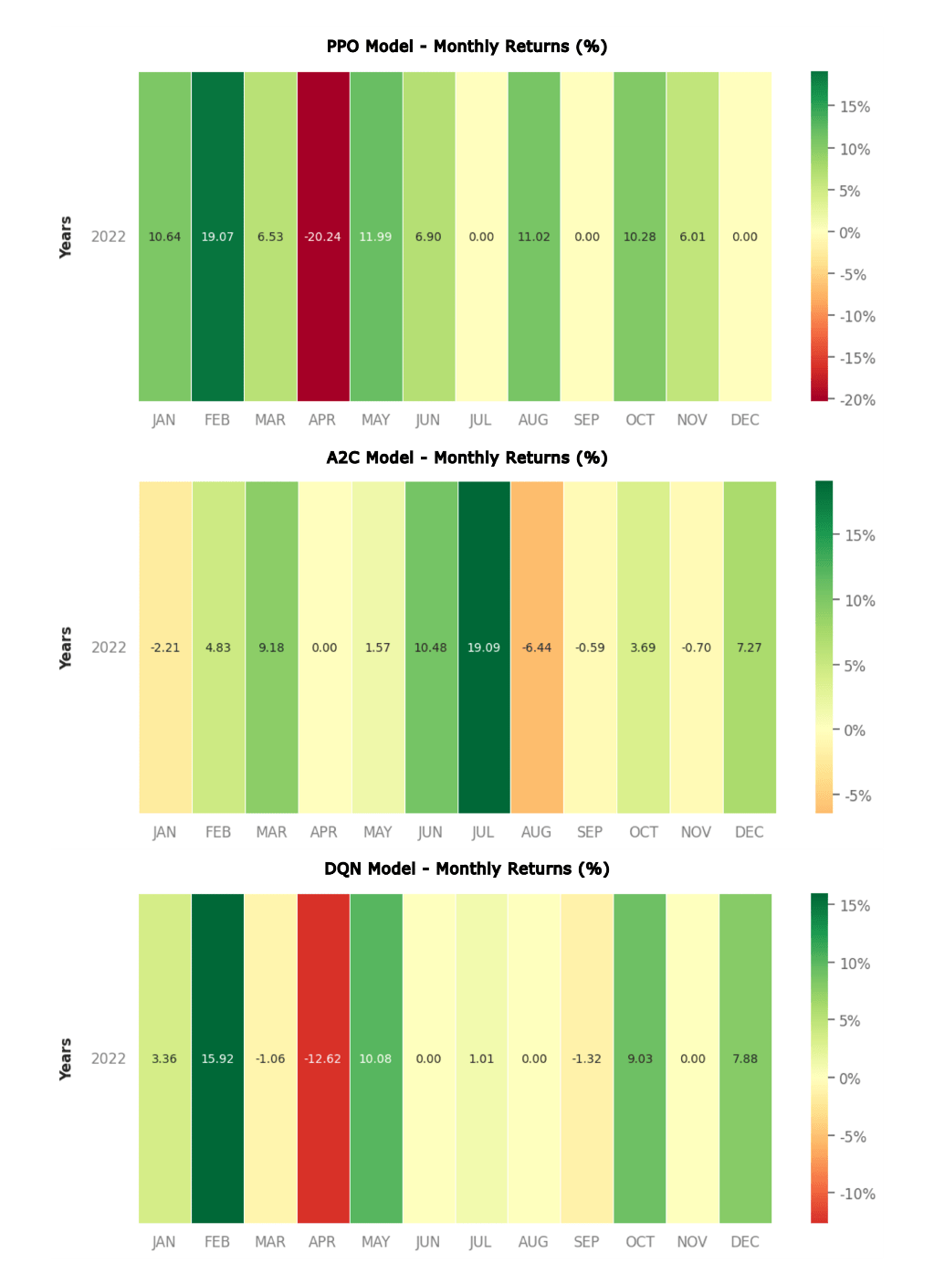
Further analysis of monthly returns puts forward the differences in consistency among models. The PPO model shows strong returns in January and February but had a notable dip in April. Despite this, the PPO model continued to make consistent positive returns and maintained a high average in monthly returns. The DQN model displayed a similar pattern, but plateaued from June to September, following a few positive return months. The A2C model showed no huge drawdowns in the monthly returns and displayed moderate returns throughout the year; nevertheless, it resulted in a lower average monthly return compared to that of the PPO model.

Risk-Adjusted Performance

	Sharpe Ratio (unitless)	Calmar Ratio (unitless)	Sortino Ratio (unitless)	Profit Factor (ratio)	Omega (ratio)
PPO Model	1.24	1.71	3.33	2.76	46
DQN Model	1.82	2.41	3.02	4.02	55.31
A2C Model	2.11	5.16	5.47	3.5	26.98

The various models were benchmarked against key financial indicators to underline risk-adjusted returns, including downside risk management and overall profitability. Indeed, the A2C model showed the best risk-adjusted performance, with a Sharpe ratio of 2.11, underlining the best balance between return and risk. This was again reflected in its Calmar ratio, standing at 5.16, far outperforming the DQN and PPO models, which had returns of 2.41 and 1.71, respectively. The same A2C was leading in the Sortino ratio, with a value of 5.47. Interestingly, the PPO model outperformed the DQN model in the Sortino ratio, reading 3.33 against 3.02, respectively. The Omega ratio is a measure used in finance to evaluate the performance of an investment by comparing the probability of returns above a certain threshold to the probability of returns below that threshold. The DQN model achieved the highest Omega ratio at 55.31, followed by the PPO model with an Omega ratio of 46. The A2C model recorded an Omega ratio of 26.98.

Profitability Metrics

The DQN model would be the most profitable, considering profitability defined as a Profit Factor of 4.02 for the highest gross profitability relative to losses. The A2C model had a Profit Factor of 3.5 and PPO of 2.76. Although the A2C stood out in risk-adjusted metrics, the higher gross profitability makes the DQN surpass others in net profit generation.

Discussion

This study evaluated three DRL models using Google’s historical stock data sourced from Yahoo Finance and accessed through DI-Engine’s AnyTrading library. The dataset includes dates, opening and closing prices, daily highs and lows, adjusted closes, and volume, though only closing prices were used for model training and evaluation. Among the three models, the PPO model achieved the highest cumulative profit return of 62%, with the A2C model following with a return of 42%. The DQN model performed the worst in terms of cumulative profit returns but still had better risk-adjusted metrics compared to the PPO. The DQN model had the highest Omega ratio of 55.31 and the highest profit factor of 4.02. The A2C model is the best in terms of risk-adjusted metrics as it led in the Sharpe ratio, Calmar ratio, and Sortino ratio, with values of 2.11, 5.16, and 5.47, respectively. 

Model Analysis

The findings from this study highlight some of the strengths and weaknesses of the DRL models. The PPO model shows the greatest potential for maximizing growth as it had a EoY return of 62%. However, this “most profitable” characterization does not mean superior efficiency on all profitability metrics. In fact, the model is more volatile compared to the others. As seen in figure 2, there was a 20.24% drop in returns during the month of April. Furthermore, the model isn’t performing up to par regarding risk-adjusted performance. The PPO model’s low Sharpe ratio of 1.24 shows that the model may not be making adequate returns despite taking greater risks. Its Calmar ratio of 1.71 further emphasizes that it is prone to experiencing significant losses during downturns, which can be detrimental during a bear market. In addition, because the PPO model’s Sortino ratio was at the lower end of the spectrum, it highlights how it may not be a favorable option for minimizing losses. This is further backed up by the model’s low profit factor of 2.76, which shows that the model experiences more frequent or larger losses compared to gains. The PPO model, however, does have a relatively high Omega ratio of 46 which shows that it is effective in generating returns over a certain threshold. This also shows that the model can be profitable in various market conditions. But due to the many lacking performance in other measures, the PPO model is likely to be the least consistent and dependable model yet despite having the greatest cumulative returns. This is further backed by Figure 3; the PPO model generated high returns in the early months but a notable drawdown during April highlighted the model’s volatility.

The DQN model displayed moderate growth potential with an EoY return of 32%. As seen in Figure 1, the DQN model was on the more volatile end of the spectrum with notable fluctuations, such as the sharp decline in April, like the PPO model, as seen in Figure 2. According to Table 1, the DQN model had a Sharpe ratio of 1.82. While this is higher than the PPO model, it still indicates that the model carries considerable risk relative to its returns. The Calmar ratio of 2.41, while again better compared to the PPO, still does not meet the standard set by the A2C model. Thus, the DQN model may still struggle during prolonged market downturns. The DQN model also had the worst Sortino ratio of 3.02 indicating that the DQN is not the best in being able to manage downside risk. Nevertheless, the model had the highest profit factor of 4.02, suggesting that it generates more profits relative to losses. The DQN model’s Omega ratio of 55.31 supports this by suggesting superior performance in achieving returns above a certain threshold. Figure 3 also showed that the DQN model had periods where gains were almost nullified by subsequent losses, revealing less consistency. Overall, the DQN model is a mixed bag with difficulties all over. For this reason, we feel that the DQN model may not be the most reliable of the three models either but may be a better alternative to the PPO.

The A2C model showed the strongest risk-adjusted performance and ended with a EoY return of 46%. It had a Sharpe ratio of 2.11 which was the highest of the 3 models, showing that the model is effective in generating more profits while limiting the risks involved. The model’s high Calmar ratio of 5.16 further shows that the model does not make significant losses during economic downturns, which is especially important when markets are bearish. Although the monthly returns heatmap (figure 2) shows moderate returns, the model’s gain is still very stable, reflecting its ability to limit significant drawdowns. The A2C model’s Sortino ratio of 5.47, which was also the highest amongst the 3 models, further highlights its strength in limiting downside volatility. The A2C model’s profit factor of 3.5, although less than that of the DQN, shows its moderate ability to balance profits and losses. Although the A2C had the lowest Omega ratio at 26.98, which suggests that it generates fewer returns above a certain threshold, the model excels in being risk-averse and consistent even during volatile market conditions. This is further supported by Figure 3, which shows more stable, moderate returns every month, in contrast to the PPO and DQN models. Although the PPO model had the greatest cumulative return, the A2C model exceled at minimizing drawdowns and sustaining positive results across the 1-year test period.

While all three models had net positive returns over the period tested, we also compared how these models performed compared to a buy-and-hold strategy as well as the S&P 500 returns over the same period. When compared to the buy-and-hold strategy, only the A2C and PPO models performed noticeable better while the DQN made almost equal returns. The A2C and PPO models return a difference of 14% and 30% respectively compared to the buy-and-hold strategy. Comparing these models to the returns of the S&P 500 index, all 3 models performed better than the index. The PPO model outperformed the index by approximately 41%, the A2C model outperformed by approximately 25%, and the DQN outperformed the index by 11%. This shows that the models can prove to be better alternatives to basic buy-and-hold strategies for both the specific asset and the general market.

Limitations and Influencing Factors

This study has a few limitations that could have influenced the results of the DRL models. One limitation is that the models were trained solely on Google’s historical stock data. Since other stocks, such as Microsoft, Apple, or Nvidia, weren’t used to train and test the DRL models, the generalizability of the models was limited. Because different stocks may be influenced by different patterns, market sentiment, and other behaviors, the DRL models may not be able to perform as well on different stocks unless trained on the stock’s historical data. Although the single-stock design was intentional to limit other confounding variables and simplify benchmarking, it limits the practical applicability of the models. Another limitation that may have influenced the DRL models’ strategy would be not incorporating transactions costs in the stock environment. This may have led the models to be more aggressive and may lead to the models being less effective in real-world scenarios. Real world phenomena such as slipping and market impact – where order execution prices differ from expected prices – were not tracked. This omission could lead to an overestimate in returns and in a more realistic environment, slippage and market impact would likely diminish the absolute profitability²¹. Additionally, the lack of information of external factors such as market sentiment, news, earnings reports, and macroeconomic indicators overlook principal factors that have a profound influence on stock price movements. This study also restricted agent actions to only 3 discrete actions: buy, sell, and hold for one share per transaction. While this feature was necessary to simplify benchmarking and track percent returns over raw profits, it does not simulate real-world trading which involve variable position sizing and portfolio rebalancing. These limitations show that these models still have room for improvement, especially if they were to be implemented in real-world trading scenarios.

Future Directions

Future research on the application of AI solutions in financial markets should prioritize a few features. The first feature would be incorporating transactional costs to make the trading environment even more realistic and thus more applicable to real-world trading. This feature may have the inadvertent effect of making the models more risk-averse and reducing the amount of mass buying/selling. Another feature that would improve the accuracy of these models is by using technical indicators such as oscillators and moving averages. This would provide additional data points for the model to utilize and identify patterns within. Future studies should also attempt to provide these models with information on market sentiments, news, earnings reports, and other macroeconomic events (e.g., rate cuts). The combination of these features would make the models extremely robust and likely extremely capable of reliably trading in the stock market. Future research should also compare these models to more basic algorithms for trading in the stock market such as mean reversion, arbitrage, moving average crossovers, and volume-weighted average price strategies.

Conclusion

In this study, we evaluated the performance of 3 DRL models – the PPO, DQN, and A2C – and compared their effectiveness in trading in the stock market. Traditional solutions and attempts to effectively trade in the stock market have been limited due to their algorithms overfitting and lack of being able to simulate real-world scenarios. In this paper, we have shown that DRL models may have the potential to replace these traditional methods while addressing the issues of overfitting and realistic scenarios. We hope that this study will lay the groundwork for future research in attempting to improve the effectiveness of DRL models in financial markets. We think that future research should focus on trying to increase the number of data points these models use when making financial decisions by utilizing technical indicators and market sentiment through the news. Another avenue for advancing this field of research would be creating an entire system of DRL models to trade by integrating a portfolio management system, quarterly/annual report analyzer, and live market trading bots. This robust ensemble has the potential to completely automate trading in financial markets.

References

1. Park, Cheol-Ho, and Scott H. Irwin. “The Profitability of Technical Analysis: A Review.” 2004. [↩]
2. Liu, Tom, Stephen Roberts, and Stefan Zohren. “Deep Inception Networks: A General End-to-End Framework for Multi-Asset Quantitative Strategies.” arXiv preprint arXiv:2307.05522, 2023. [↩]
3. Arulkumaran, Kai, et al. “Deep Reinforcement Learning: A Brief Survey.” IEEE Signal Processing Magazine, vol. 34, no. 6, 2017, pp. 26-38. [↩]
4. Yi, Shicheng. “Behavioral Finance: Several Key Effects of Investor Decision-Making.” SHS Web of Conferences, 2024. [↩]
5. Pricope, Tidor-Vlad. “Deep Reinforcement Learning in Quantitative algorithmic Trading: A Review.” arXiv preprint arXiv:2106.00123, 2021. [↩]
6. Mohan, Saloni, et al. “Stock Price Prediction Using News Sentiment Analysis.” 2019 IEEE Fifth International Conference on Big Data Computing Service and Applications (BigDataService), IEEE, 2019. [↩]
7. Tripathy, Naliniprava. “Stock Price Prediction Using Support Vector Machine Approach.” Indian Institute of Management, 2019. [↩]
8. Wu, Yifan. “Stock Price Prediction Based on Simple Decision Tree Random Forest and XGBoost.” EMFRM, vol. 38, 2023, pp. 3383-3390. [↩]
9. Fjellström, Carmina. “Long Short-Term Memory Neural Network for Financial Time Series.” arXiv preprint arXiv:2201.08218, 2022. [↩]
10. Aadhitya, A., et al. “Predicting Stock Market Time-Series Data using CNN-LSTM Neural Network Model.” arXiv preprint arXiv:2305.14378, 2023. [↩]
11. Chen, Zhengting. “Research on Portfolio Optimization Model based on Machine Learning Algorithm in Stock Market.” Transactions on Economics, Business and Management Research, 2024. [↩]
12. Sakilam, Abhiman, et al. “Deep Reinforcement Learning Algorithms for Profitable Stock Trading Strategies.” 2024 IEEE International Conference on Contemporary Computing and Communications (InC4), vol. 1, 2024, pp. 1-6. [↩]
13. Zhang, Nan, et al. “Deep Reinforcement Learning Trading Strategy Based on LSTM-A2C Model.” Other Conferences, 2022. [↩]
14. de la Fuente, Neil, and Daniel Vidal. “DQN VS PPO VS A2C: Performance Analysis in Reinforcement Learning.” arXiv preprint arXiv:2407.14151, 2024. [↩] [↩] [↩]
15. Xiao, Xiaochen, and Weifeng Chen. “A Model for Quantifying Investment Decision-making Using Deep Reinforcement Learning (PPO Algorithm).” Advances in Economics, Management and Political Sciences, 2023. [↩]
16. A Novel Deep Reinforcement Learning Based Automated Stock Trading System Using Cascaded LSTM Networks.” Expert Systems with Applications, vol. 242, 2024, p. 122801. [↩]
17. Benhamou, Eric, et al. “Omega and Sharpe Ratio.” Mutual Funds, 2019. [↩] [↩]
18. Kidd, Deborah, and Boyd Watterson. “The Sortino Ratio: Is Downside Risk the Only Risk that Matters?” 2011. [↩]
19. Magdon-Ismail, Malik, and Amir F. Atiya. “Maximum Drawdown.” Capital Markets: Asset Pricing & Valuation, 2004. [↩]
20. Rahmah, Iin Fadillah, et al. “Profitability Ratio Analysis to Assess the Financial Performance.” International Journal of Applied Finance and Business Studies, 2024. [↩]
21. “Transaction Cost Analysis: Slippage and Market Impact.” FinchTrade Financial Glossary, 2024. [↩]