
Abstract
Chronic migraines are a neurological disorder affecting 1-2.2% of the global population1. There are many different types of migraines that people may experience. The seven classes of migraines (0-6 respectively)–migraine with aura, migraine without aura, basilar-type aura, sporadic hemiplegic migraine, familial hemiplegic migraine, typical aura without migraine, and other migraines–were considered. The objective of this study is to do an analysis on data bias seen in migraine studies by classifying seven subtypes of migraines using random forest (RF) and artificial neural network (ANN) machine learning models through Python. Nine different random forest machine learning models were created ranging in test-train splits from 35%:65% to 75%:25%. Data analysis included: precision, recall, F1-score, confusion matrices, and feature importance of the attributes considered in the initial data. The results of this study indicate that there was data bias within the initial dataset as patients, particularly in classes 2, 3, 4, and 5 as they were consistently insufficiently classified. These results suggest that data bias in migraine studies may contribute to disparities in clinical care, underscoring the need to decrease bias by including similar numbers of patients with each type of migraine being studied.
Keywords: Migraine, Migraine with aura, Migraine without aura, Basilar-Type Aura, Hemiplegic Migraine, Sporadic Hemiplegic Migraine, Familial Hemiplegic Migraine, Data bias
Introduction
Chronic migraines are defined as experiencing 15 headaches a month, 8 of which are migraines, for at least 3 months1. There are many different types of migraines and different subtypes require tailored treatments.
This study focuses on classifying seven migraine subtypes: migraine with aura (MWA), migraine without aura (MWoA), basilar-type aura (BTA), sporadic hemiplegic migraine (SHM), familial hemiplegic migraine (FHM), typical aura without migraine, and other migraines.
Migraines are clinically diagnosed—meaning diagnosed based on symptoms2. There are some symptoms such as the sensitivity to light and sound that are present in all types of migraine, but others like loss of consciousness in FHM and SHM or lack of coordination in BTA are specific to certain types of migraines3,4. Being significantly less common though, people affected by these types of migraines make up only a narrow proportion within medical studies. This results in less awareness of symptoms in both patients and physicians. The dataset in this study is derived from Kaggle and consists of 400 patients with 24 different clinical attributes5. These range from the character of their migraine to specific symptoms such as ataxia (lack of coordination)6. Patients in the data were diagnosed with one of the seven subtypes previously stated. Addressing data bias in migraine classification is crucial to improving diagnostic accuracy and ensuring patients with rare types of migraines are accurately diagnosed and treated appropriately7.
The primary aims of this paper are as follows:
- To assess data bias within this dataset and which factors most influence the classification of migraine types
Literature Review
Migraines rely on a clinical diagnosis meaning that physicians diagnose patients based on symptoms that they display. As it is a clinical diagnosis, there are no scans that can be used to assess whether a person has a migraine and what type of migraine they have. Although migraines share common symptoms such as throbbing pain, discomfort, and vomiting, there are also some symptoms that are unique to specific types of migraines.
This study will look at seven different types of migraine: MWA, MWoA, BTA, SHM, FHM, other types of migraines, and typical aura without migraine. The National Institute of Neurological Disorders and Stroke defines MWA as a type of migraine accompanied with spots and zigzags as well as the broader symptoms like throbbing pain and vomiting3.
There are also different types of migraine with aura, such as brainstem aura (BTA), and hemiplegic aura. Basilar type aura consists of vertigo, double vision, poor muscle coordination, slurred speech, ringing in ears, hearing loss, and fainting. A patient must display at least two distinct symptoms to be diagnosed with basilar type aura3,8.
Hemiplegic migraines in contrast consist of paralysis, specifically on one side of the body4. These symptoms are often mistaken for strokes causing many patients to be misdiagnosed9. There are two types of hemiplegic migraines: FHM and SHM. FHM is a result of mutations in genes causing an overproduction of glutamate, an excitatory neurotransmitter10. This causes the nerves in the brain to become overexcited, leading to familial hemiplegic migraine, passed down by family members. On the contrary, SHM is a random result of mutations, and this is not passed down within families4. These are the most significantly rare types of migraines, affecting only 0.01% of the population4.
There have been many studies that focus on migraine classification with the use of machine learning models. Notably, many of these studies use the same publicly available dataset from Kaggle of 400 patients with 24 attributes including frequency, intensity, and location5.
Khan et al.11 focuses on classifying different types of migraines using five different types of machine learning models to determine which is most accurate in predicting types of migraines. It uses a support vector machine (SVM), K-nearest neighbors (KNN), a random forest model (RF), a decision tree (DST), and deep neural network algorithms (DNN), to classify the different types of migraines within the dataset based off their attributes. From the initial 400 patients, the data was augmented to 1447 to balance the ratios of the patients diagnosed with each type of migraine. Results indicated that the DNN model was the most accurate in predicting types of migraines after the data was augmented with 99.66% accuracy. Limitations of this study included the subjective pain intensity ratings as well as the fact that migraines are a complex neurovascular disorder meaning that a machine learning model will not be able to always accurately predict the type of migraine a patient has.
Reddy et al.12 used different types of machine learning models to determine which was best at predicting different types of migraines based off attributes. A logistic regression (LR) model, SVM, RF, and artificial neural network (ANN) model were used. The study used a fixed train-test split of 0.8:0.2 and used the area under an ROC curve, classification report, precision, recall, and specificity score to determine which model was most accurate in classifying specific types of migraines. This study ran each model with random sampling and selective sampling. Random sampling allows all patients to have an equal chance in representation within the study. There is low bias when studies are conducted with random sampling as there is no specific type of patient being assessed. Selective sampling, in contrast refers to when patients are picked to be represented in a study based off specific characteristics. This results in high bias and low representation. When run with random sampling, results indicated that the ANN and SVM models were more accurate in their prediction with precision and accuracy scores of 91%. When conducting machine learning models with selective sampling, the accuracy of each model increased. LR increased from 90% to 95%, RF increased from 87% to 98%, ANN increased from 91% to 99%, and SVM increased from 91% to 96%. The results of this study indicate ANN to be the most precise in classifying types of migraines with RF and SVM models to be reliable alternatives.
Filippis et. al13 assessed if AI-driven methods were more beneficial in classifying different types of migraines. The study compared the results of AI classification to the classification of various machine learning models including DST, RF, and SVM. There was a fixed train: test split of 80:20. The study used the same dataset as the studies previously mentioned as well as the dataset that is used in this study, consisting of 400 patients and 24 different attributes including frequency, intensity, and location. Results were determined with the use of an accuracy score, precision, recall, and F1-score, as well as a confusion matrix and correlation matrix. This determined correlations among symptoms for all migraines (symptoms that all migraines share), and well as negative correlations (symptoms that are specific for some types of migraines).
While previous studies focus on optimizing the most accurate machine learning model to classify types of migraines, the current research aims to investigate data bias within migraine classification sets. Data bias occurs when a dataset of disproportionately factors or underrepresents certain elements, leading to inaccurate predictions. It is important for medical datasets to be as unbiased as possible to ensure proper diagnoses and treatment for patients7,14.
Methods
Random Forest
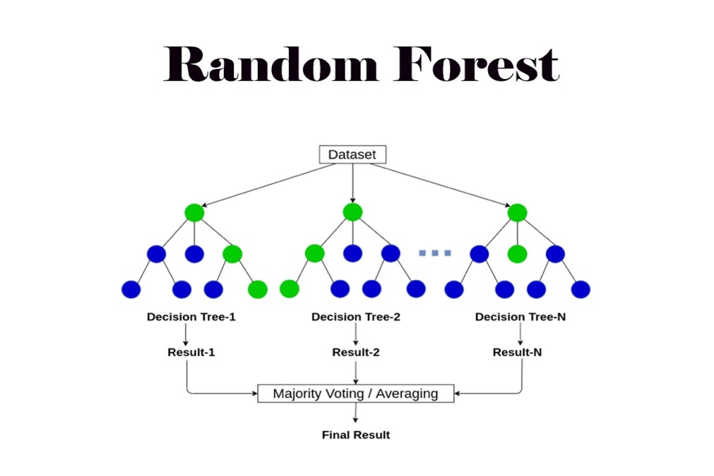
The machine learning model in this study was built with a random forest. Random forests are built from decision trees, each trained on a subset of data.15
. Decision trees are not flexible when it comes to adding new samples whereas random forests combine the simplicity of decision trees with flexibility resulting in a vast improvement in accuracy16. A random forest classification model was generated to determine how well the machine learning model is at predicting the different types of migraine based on given attributes. The RF model was trained using a Random Forest Classifier. This allows each decision tree to be trained with a random subset of the training data, which improves robustness and diversity among the trees. A random state of 42 was also used to train the model. This makes sure that the randomness of the model will yield the same results each time it is run15,16.
Figure 1 provides an illustration of a random forest model.
Artificial Neural Network Model
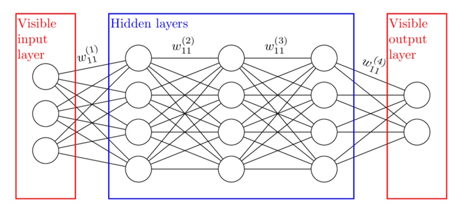
An artificial neural network model is used to help predict and forecast different complex systems. It is helpful when trying to predict relationships between variables by mimicking a human working brain18. This type of model has been very beneficial and accurate in predicting types of migraines based on clinical factors. When designing the ANN model, a random state of 42 was also used to make sure that the randomness of the model will yield the same results each time it is run. ANN models also use hidden layers. This is a layer of artificial neurons where the neural network processes the information between the input and output. The ANN model in this study had an input later of 23 attributes (all except the type of migraine). The first hidden layer had 64 neurons, each neuron learns patterns from the raw features. The second hidden layer was 32 neurons which processes the outputs from the first layer even further. The output layer was 7 neurons, one for each of the seven classes. Figure 2 provides an illustration of how each layer of an ANN model works.
Data
The sample used in this study consisted of 400 patients, each diagnosed with a migraine. Specifics of each migraine episode like its duration and frequency were considered. Attributes of the migraine like location and intensity were also included in the dataset. The dataset also consisted of many symptoms common with migraines like vomiting and nausea, and neurological symptoms like photophobia and phonophobia6. The ANN and RF models were trained and evaluated across nine train-test split configurations.
Class Composition
There were seven different classes of migraines that were generated in the machine learning model. Class 0 consisted of patients who had MWA. Class 1 consisted of patients who had MWoA. Class 2 consisted of patients with BTA. Class 3 consisted of patients with SHM. Class 4 consisted of patients with FHM. Class 5 consisted of patients with other migraines, none that were already being accounted for. Class 6 consisted of patients who had a typical aura without migraine. Performance was assessed using the precision, recall, and F1-score per class. Table 1 shows the division of patients within the dataset, highlighting the class imbalance in the dataset.
| Class | Type of Migraine | Number of patients diagnosed |
| 0 | MWA | 247 |
| 1 | MWoA | 60 |
| 2 | BTA | 18 |
| 3 | SHM | 14 |
| 4 | FHM | 24 |
| 5 | Other migraines | 20 |
| 6 | Typical aura without migraine | 17 |
Attribute Ratings
Patients were asked to rate many of their attributes with numerical values that are explained in Table 2.
| Attribute | Definition | Scoring |
| Age | Patient’s age | |
| Duration | Duration of symptoms in last episode in days | |
| Frequency | Frequency of episodes per month | |
| Location | Unilateral or bilateral pain location | (None – 0, Unilateral –1, Bilateral – 2) |
| Character | Throbbing or constant pain | (None – 0, Throbbing – 1, Constant – 2) |
| Intensity | Pain intensity, i.e., mild, medium, or severe | (None – 0, Mild – 1, Medium – 2, Severe – 3) |
| Nausea | Nauseous feeling | (No – 0, Yes – 1) |
| Vomit | Vomiting | (No – 0, Yes – 1) |
| Photophobia | Noise sensitivity | (No – 0, Yes – 1) |
| Visual | Number of reversible visual symptoms | |
| Sensory | Number of reversible sensory symptoms | |
| Dysphasia | Lack of speech coordination | (No – 0, Yes – 1) |
| Dysarthria | Disarticulated sounds and words | (No – 0, Yes – 1) |
| Vertigo | Dizziness | (No – 0, Yes – 1) |
| Tinnitus | Ringing in the ears | (No – 0, Yes – 1) |
| Hypoacusis | Hearing loss | (No – 0, Yes – 1) |
| Diplopia | Double vision | (No – 0, Yes – 1) |
| Visual defect | Simultaneous frontal eye field and nasal field defect in both eyes | (No – 0, Yes – 1) |
| Ataxia | Lack of muscle control | (No – 0, Yes – 1) |
| Conscience | Jeopardized conscience | (No – 0, Yes – 1) |
| Paraesthesia | Simultaneous bilateral paraesthesia | (No – 0, Yes – 1) |
| DPF | Family background | (No – 0, Yes – 1) |
| Type | Diagnosis of Migraine Type | (Typical aura with migraine, Migraine without aura, Typical aura without migraine, Familial hemiplegic migraine, Sporadic hemiplegic migraine, Basilar-type aura, Other) |
Data preprocessing
The software Python 3 (ipykernel) in Jupyter Notebook was used to generate the machine learning model used in this paper. The data was initially cleaned within Jupyter Notebook, making sure to eliminate all rows with missing values. This was an important factor to ensure that the data that was used all had responses regarding each of the attributes to ensure predictions were as accurate as possible.
| X_train | The feature data for the training set |
| X_test | The feature data for the test set |
| Y_train | The label data for the training set |
| Y_test | The label data for the test set |
Table 3 defines the dependent and independent variables of the dataset within the machine learning model. The feature data refers to the attributes within the dataset, and the label data refers to the type of migraine. The data was then split into the training and test sets from a test-train splits of 35:65 to 75:25. The RF and ANN were generated by fitting the model to the training data. This is when the model trains itself with the training data to be able to predict the types of migraines based on the attributes provided by the testing data. The machine learning models then predicted on the testing data using the model.
Varying Train-Test Splits
The current study focuses on varying train-test splits from 65:35 to 25:75. This was done as a robustness check – to determine if performance is stable or highly sensitive to sample size. It was also done to accommodate for the rarer classes like SHM and FHM. With less patients in these classes, they may be underrepresented in a test set at certain splits. Varying train-test splits are important to help determining when and why the model fails on those classes, especially in small and imbalanced datasets.
Performance Metrics
Precision, Recall, and the F1-score are pivotal metrics to understand classification models such as these. There are four metrics that are measured with these metrics: true positives (TP), true negatives, (TN), false positives (FP), and false negatives (FP)20,21. TP show instances where the machine learning model accurately predicted the data to correspond to its respective class20,21. TN similarly show instances where the machine learning model accurately predicted the data to correspond to whichever class it did not belong to20,21. FP show when the machine learning model predicted data into a class it did not belong to, and FN show when the machine learning model was ineffective in accurately predicting data to a class it did not belong to20,21. All these metrics were recorded for each machine learning model in this study (35%-75%). The precision of a model measures the accuracy of a model’s positive predictions, meaning its TP and FP20. Recall measures how often a model correctly identifies the true positive rate (the proportion of actual positive cases that are identified by the model)20. The F1-score balances the recall and precision of a model to identify the model’s performance and overall, it’s accuracy20. All three of these factors are important to help determine the efficacy of the model.
Confusion matrices show how well a machine learning model predicts data by comparing predicted values to actual values. They consisted of four groups: TP, TN, FP, and FN21. Confusion matrices were computed for the 9 machine learning models to compare each of their performance. Each matrix provided a class-by-class breakdown which helps understand whether there is bias within the data.
Statistical Approach
To determine data bias within the dataset, an ANOVA test was performed. The purpose of this was to evaluate statistically significant differences between the different classes22. Before performing the test, it is crucial to make sure assumptions are met. These include normality, homogeneity or variance, independence, and random sampling23. Normality refers to when data points cluster around a central value23. The ANOVA is created to compare 7 groups in this study. Each group as well as how many patients are being represented within each is shown in Table 4 below
| Type of Migraine | Number of patients diagnosed |
| MWA | 247 |
| MWoA | 60 |
| BTM | 18 |
| SHM | 14 |
| FHM | 24 |
| Other migraines | 20 |
| Typical aura without migraine | 17 |
Kernel Density Estimation plots (KDE) were created for each of the attributes within the data to determine whether there was normality. Figure 3 shows the KDE plots created for intensity across the seven migraine subtypes.
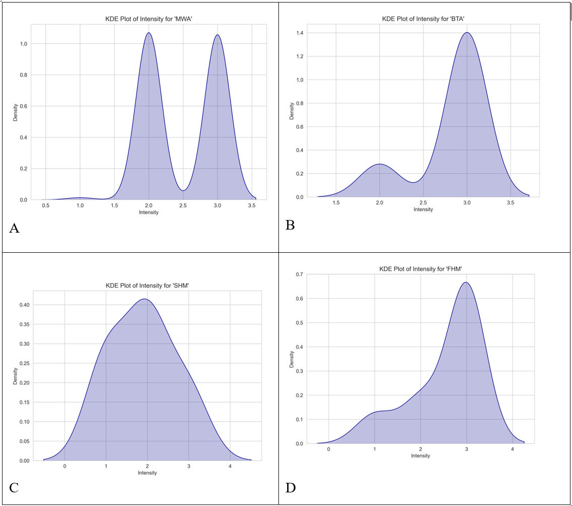
Figures 3A, 3B, 3C, and 3D are all negatively skewed meaning that they do not achieve normality. All the attributes in this dataset did not achieve normality either meaning that an ANOVA would not be suitable. Instead, a Kruskal-Wallis (H-statistic) test was run. The purpose of this is to determine whether there are statistically significant differences between the medians of the attributes within the seven different groups of migraines24. Figure 4 shows the equation to find the H statistic, which measures the differences between the means of the groups, to solve for a Kruskal-Wallis test.

The Kruskal-Wallis tests were all generated and run within Python. If there was a p-value less than 0.05, a significant difference was detected between at least one group. When comparing the attribute intensity of patients between the seven migraine groups, the H statistic computed was 19.3202, while the p-value was 0.0037 meaning that a significant difference was detected between at least one group. Out of the 24 attributes, 23 (all except for type), resulted in a significant difference between at least one group. Figure 5 shows the result for attribute ‘intensity’ across the 7 migraine types from the Kruskal-Wallis test.

Dunn’s tests were then run to determine which groups had a significant different24. Data was cleaned eliminating all rows and columns with missing values. After this, the Dunn results for ataxia were skipped due to having too many missing values. 22 Dunn’s tests were computed and every attribute had significant pairs. Table 5 shows the Dunn’s test results for intensity.
| Basilar-type aura | Familial hemiplegic migraine | Migraine without aura | Other | Sporadic hemiplegic migraine | Typical aura with migraine | Typical aura without migraine | |
| Basilar-type aura | 1.0 | 0.9426323718879860 | 1.0 | 1.0 | 0.06335654466588580 | 0.058965376605843500 | 2.8655248550662E-13 |
| Familial hemiplegic migraine | 0.9426323718879860 | 1.0 | 0.012169478139298700 | 0.18372648313619700 | 1.0 | 1.0 | 1.21020172865987E-08 |
| Migraine without aura | 1.0 | 0.012169478139298700 | 1.0 | 1.0 | 0.0004409321289196620 | 1.71326140661475E-09 | 2.12247353853189E-24 |
| Other | 1.0 | 0.18372648313619700 | 1.0 | 1.0 | 0.009825137369418290 | 0.0040260673670928400 | 4.77463749565627E-15 |
| Sporadic Hemiplegic Migraine | 0.06335654466588580 | 1.0 | 0.0004409321289196620 | 0.009825137369418290 | 1.0 | 1.0 | 0.0007114898880640200 |
| Typical aura with migraine | 0.058965376605843500 | 1.0 | 1.71326140661475E-09 | 0.0040260673670928400 | 1.0 | 1.0 | 5.23219175117759E-13 |
| Typical aura without migraine | 2.8655248550662E-13 | 1.21020172865987E-08 | 2.12247353853189E-24 | 4.77463749565627E-15 | 0.0007114898880640200 | 5.23219175117759E-13 | 1.0 |
For further breakdown, Table 6 shows which groups have significant differences.
| Group 1 | Group 2 | P-value | Significant? |
| Migraine without aura | Typical aura without migraine | 2.12e-24 | Yes |
| Other | Typical aura without migraine | 4.77e-15 | Yes |
| Basilar-type aura | Typical aura without migraine | 2.87e-13 | Yes |
| Typical aura with migraine | Typical aura without migraine | 5.23e-13 | Yes |
| Migraine without aura | Typical aura with migraine | 1.711e-09 | Yes |
| Familial hemiplegic migraine | Typical aura without migraine | 1.21e-08 | Yes |
| Migraine without aura | Sporadic hemiplegic migraine | 4.411e-04 | Yes |
| Sporadic hemiplegic migraine | Typical aura with migraine | 7.11e-04 | Yes |
| Other | Typical aura with migraine | 4.03e-03 | Yes |
| Other | Sporadic hemiplegic migraine | 6.34e-02 | Yes |
| Familial hemiplegic migraine | Migraine without aura | 1.22e-02 | Yes |
| Basilar-type aura | Typical aura with migraine | 5.90e-02 | No |
| Basilar-type aura | Typical aura with migraine | 6.34e-02 | No |
| Familial hemiplegic migraine | Other | 1.84e-01 | No |
| Basilar-type aura | Familial hemiplegic migraine | 9.43e-01 | No |
| Sporadic hemiplegic migraine | Typical aura with migraine | 1.0 | No |
| Migraine without aura | Other | 1.0 | No |
| Basilar-type aura | Other | 1.0 | No |
| Basilar-type aura | Migraine without aura | 1.0 | No |
| Familial hemiplegic migraine | Typical aura with migraine | 1.0 | No |
The Dunn’s test for intensity revealed statistically significant results between Typical aura without migraine and many other types of migraine including MWoA (p=2.12e-24), and other (p=4.77e-15). This suggests that Typical aura without migraine is clinically distinct compared to the other types of migraine. In contrast, comparison between FHM and MWA (p=1.0) is not. See appendices A and B for additional results of other attributes.
Data and Analysis
Classification Report
Each classification report of this study showed the precision, recall, F-1 score, and support of each machine learning model. The support shows how many patients within each class were assessed corresponding for the train: test proportion. Tables 7 and 8 illustrate the classification reports for each ANN and RF machine learning model with the test-train split 35:65. The weighted averages of the recall, precision, and F-1 scores are shown in each Table. This data was used to create illustrations of the class performances for each machine learning model.
| Class | Precision | Recall | F1-score | Support |
| 0 | 0.89 | 0.98 | 0.93 | 87 |
| 1 | 0.95 | 1.00 | 0.98 | 21 |
| 2 | 0.75 | 0.50 | 0.60 | 6 |
| 3 | 0.75 | 0.60 | 0.67 | 5 |
| 4 | 0.25 | 0.12 | 0.17 | 8 |
| 5 | 1.00 | 0.50 | 0.67 | 6 |
| 6 | 1.00 | 1.00 | 1.00 | 7 |
| Accuracy | 0.88 | 140 | ||
| Macro avg | 0.80 | 0.67 | 0.72 | 140 |
| Weighted avg | 0.86 | 0.88 | 0.86 | 140 |
| Class | Precision | Recall | F1-score | Support |
| 0 | 0.92 | 0.94 | 0.93 | 87 |
| 1 | 0.88 | 1.00 | 0.93 | 21 |
| 2 | 0.83 | 0.83 | 0.83 | 6 |
| 3 | 0.40 | 0.40 | 0.40 | 5 |
| 4 | 0.60 | 0.38 | 0.46 | 8 |
| 5 | 1.00 | 0.67 | 0.80 | 6 |
| 6 | 1.00 | 1.00 | 1.00 | 7 |
| Accuracy | 0.89 | 140 | ||
| Macro avg | 0.80 | 0.75 | 0.77 | 140 |
| Weighted avg | 0.88 | 0.89 | 0.88 | 140 |
Within both models, classes 3 and 4 performed extremely poorly. The RF model had an F-1 score of 67% and 17% for classes 3 and 4 respectively while the ANN model had an F-1 score of 40 and 46%. Although the ANN performed significantly better on all the other classes, the recall scores of classes 3-5 for both models were tremendously low. This means that overall, both models were not sufficient in correctly predicting the types of migraines based on the attributes. The precision scores also show that both models were insufficient at correctly predicting whether patients had class 3 and 4 migraines based on their given attributes. Figure 6 shows the confusion matrices for both machine learning models for the 35:65 test-train split. The purpose of this is to establish what different classes were misclassified to be by the machine learning models.
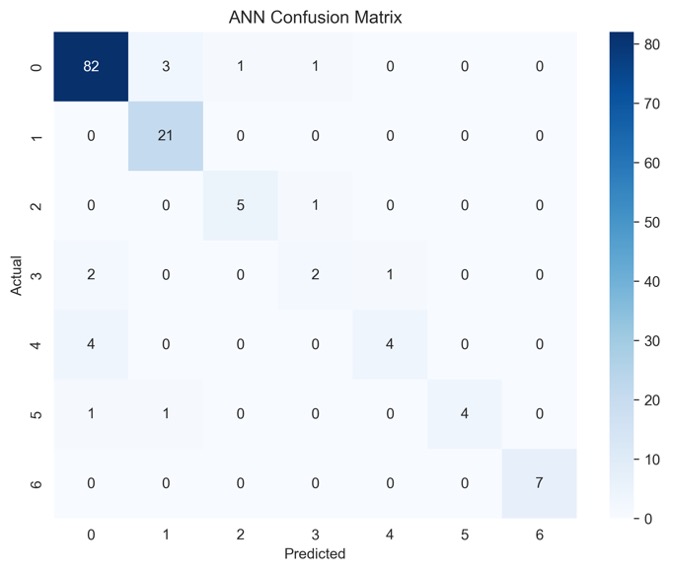

The matrices indicate that there is class bias within the dataset, as the highest proportion of data consists of patients in class 0. Figure 6 gives a more detailed look into the TP, TN, FP, and FN of each machine learning model. Figure 6A shows that the ANN model misclassified patients in class 3 as patients in class 0 and 4. Figure 6B shows that most misclassifications for class 4 were in class 0. To follow up, Figure 7 displays the class-wise misclassifications of each model. Using the data derived from the confusion matrices, the class-wise misclassification graphs show the accurate and inaccurate predictions in each class.
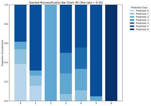
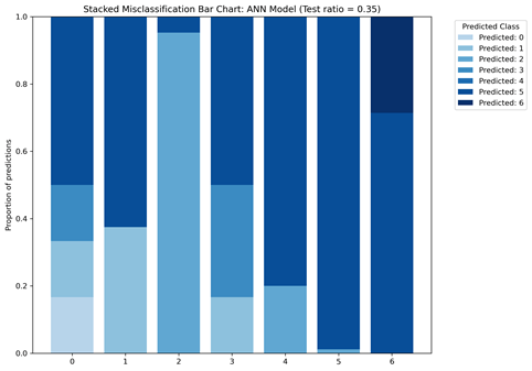
The class-wise misclassification charts are helpful in understanding which classes the machine learning models mistook certain classes for based on their given attributes. It takes the data for confusion matrices to generate a bar graph showing the misclassifications. Figures 7A and 7B both show that for class 6, there were no incorrect predictions. It also shows that the RF model was more successful in predicting patients in class 0 (proportion of predictions=0.4) compared to the ANN model (proportion of predictions~0.2)
While generating the machine learning models, the ANN model eventually stopped predicting the types of migraines once the test-train split increased to 60:40. As there was a significantly greater number of patients in class 0, this resulted in patients in class 1-6 to be overshadowed. Tables 9 and 10 show the results for the classification reports of the test-train split.
| Class | Precision | Recall | F1-score | Support |
| 0 | 0.87 | 0.98 | 0.92 | 148 |
| 1 | 0.92 | 1.00 | 0.96 | 36 |
| 2 | 0.83 | 0.45 | 0.59 | 11 |
| 3 | 0.67 | 0.25 | 0.36 | 8 |
| 4 | 0.56 | 0.33 | 0.42 | 15 |
| 5 | 1.00 | 0.50 | 0.67 | 10 |
| 6 | 1.00 | 1.00 | 1.00 | 12 |
| Accuracy | 0.88 | 240 | ||
| Macro avg | 0.84 | 0.65 | 0.70 | 240 |
| Weighted avg | 0.86 | 0.88 | 0.86 | 240 |
| Class | Precision | Recall | F-1 score | Support |
| 0 | 0.62 | 1.00 | 0.76 | 148 |
| 1 | 0.00 | 0.00 | 0.00 | 36 |
| 2 | 0.00 | 0.00 | 0.00 | 11 |
| 3 | 0.00 | 0.00 | 0.00 | 8 |
| 4 | 0.00 | 0.00 | 0.00 | 15 |
| 5 | 0.00 | 0.00 | 0.00 | 10 |
| 6 | 0.00 | 0.00 | 0.00 | 12 |
| Accuracy | 0.62 | 240 | ||
| Macro avg | 0.09 | 0.14 | 0.11 | 240 |
| Weighted avg | 0.38 | 0.62 | 0.47 | 240 |
The RF model for the test-train split of 60:40 shows that there was an insufficiency in predicting migraine classes 2-5 as F1-scores were below 80% for each of them. Although the overall accuracy of the model was 88%, the macro average of the recall was 65% meaning that the model was not successful in predicting correct cases. The recalls for classes 2-5 were also all significantly below 80%. Once the test split increased to 60% though, the ANN model was no longer able to predict types of migraines based on given attributes. As a result, the test-train splits 60:40=75:25 generated no results for classes 1-6. Instead, the model incorrectly classified all other patients as ones in class 0 but continued to accurately predict cases of class 0 migraines (recall=1.00). Figure 8 also shows the confusion matrices generated for each model for the 60:40 test-train split.
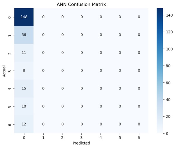

Figure 8 highlights the TP, TN, FP and FN of each machine learning model. For example, Figure 8A shows that the ANN model was able to classify all 148 patients in class 0 correctly but also predicted all subsequent classes as class 0. Figure 8B shows more variation in comparison to 8A. For example, patients in class 4 that were not correctly identified were identified as patients in classes 0 and 1. See appendices C and D for additional results of other test-train splits.
Class Bias
Based on the results from the class performance metrics and confusion matrices, it can be established that there is data bias in this dataset. In this case, this dataset is meant to represent patients with MWA, MWoA, BTA, SHM, and FHM, but it disproportionally represents patients with MWA and MWoA.
BTM, SHM, and FHM are rarer types of migraines, affecting 1.5%, and 0.01% of people respectively, whereas MWA and MWoA are more common types of migraines affecting 30% and 75% of people respectively (1,4,7). As a result, this dataset clearly does not represent patients with BTM, SHM, and FHM well. The results of the machine learning models were further analyzed to determine which attributes made up the greater 75% of the overall importance for predictions. Figure 9 displays the feature importance for both the ANN and RF models.
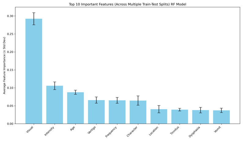
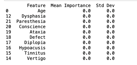
Symptoms like visual, intensity, and age made up the top three features of importance for classification in the RF model across all the test-train split. The ANN model shows that across all the test-train splits, there is no mean importance for any of the features. This means that there is no greater influence of one feature on the model’s classification compared to another. These are symptoms that are commonly seen in almost all patients who are diagnosed with migraines. Other symptoms like hypoacusis, ataxia, and diplopia are more prevalent in patients with BTA, SHM, and FHM compared to those to have MWA and MWoA.
Further analysis into feature importance was done with the use of permutation feature importance. This method looks at how much each feature influences the predictions of the model when it is randomly shuffled [26]. As there was no result for feature importance for the ANN model, no permutation feature importance could be computed for it. The results for the RF model were compared to a computed baseline of 86.4. Figure 10 shows the permutation feature importance results for the RF model.
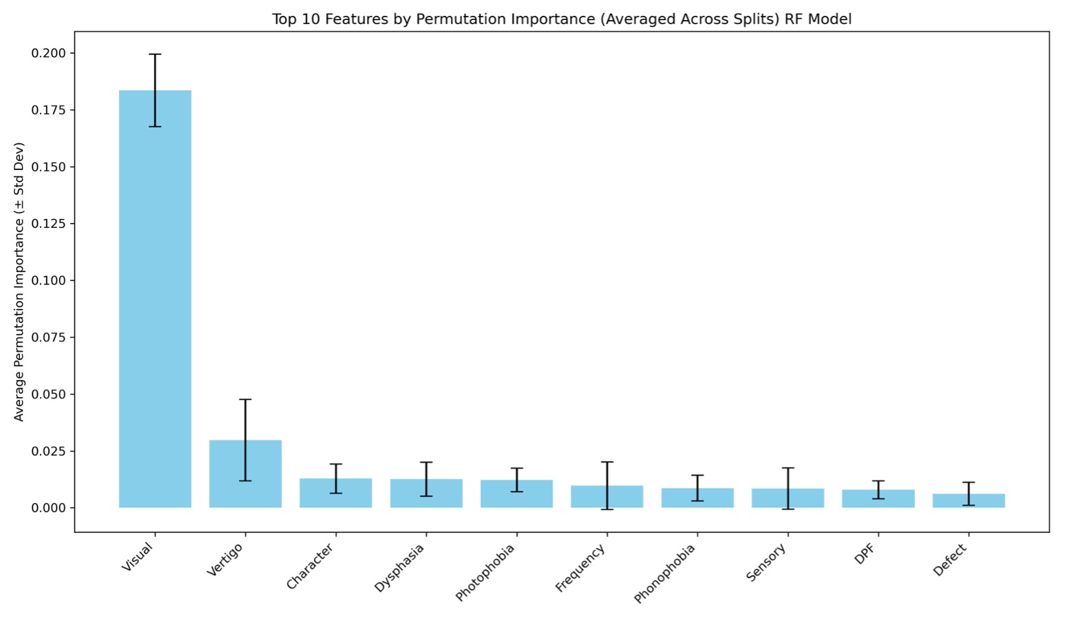
Against the baseline of 86.4, the attribute ‘Visual’ had the greatest influence on the predictions of the RF model. This means that when randomly shuffled, this attribute can influence results by ~17.2% to 20%. This means that this attribute has a 69.2% to 100.4% influence on the model’s results. Vertigo is the second most important feature, which has an influence of about ~1.6% to 5%. The attributes following vertigo (character-sensory), have low importance while DPF and Defect have little to no importance. Overall, the attribute ‘Visual’ was very influential in each model’s results. Figure 11 shows a heatmap for showcasing all 23 attributes and how they impacted classification of migraines in the RF model.
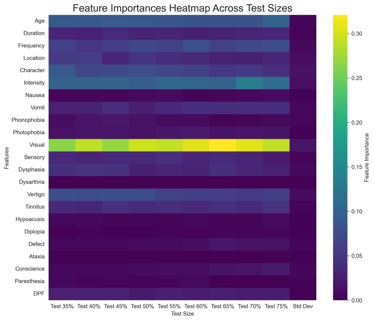
the RF model
According to the heat map, features that had the least importance on classification included (but is not limited to): hypoacusis, diplopia, ataxia, nausea, paresthesia, and conscience. Of these, symptoms that are specific to rarer types of migraine were less important when it came to the classification of migraines. Most notable is ataxia. This feature had no importance and had no results in the Kruskal-Wallis test because of too few values. Symptoms such as these are important and differentiate BTA, SHM, and FHM from more common types of migraine. The heatmap shows that these symptoms were of little importance across all the test sizes. This impacted the way the RF model classified migraines as there was not enough information in the initial dataset to help prioritize the symptoms of rarer types of migraines.
Discussion
Limitations
The weighted average of the F1-score for each machine learning model was above 80% showing that the models were sufficient in predicting classes based on given attributes. There was still a disproportionality in both the initial data and the results regarding the number of patients in classes 2, 3, 4, and 5, and how many were accurately predicted. Most of the patients in the initial dataset were patients with MWA and MWoA, the most common types of migraines. The sample size of this study was relatively small and within that, 62% of the sample consisted of patients in a single class (0). The basis of the predictions in each machine learning model were then established based on the larger sample, which is why broad attributes like visual, intensity, and frequency, that are common in MWA, made up most of the important features that were used for predictions while less common attributes like diplopia (double vision), ataxia (lack of muscle control), and dysarthria (disarticulated sounds and words), more common in SHM, FHM, and BTA made up almost none of top 10. The data also being self-reported is also a limitation as self-reports can unintentionally skew data because of patient comfort and what they are willing to reveal.
Implications
While the machine learning model was able to consistently predict the classifications for some classes, the results of this study indicate data bias. This is important to acknowledge as such bias can lead to improper care for patients. As the initial dataset had a significantly greater proportion of patients with class 0 and 1 migraine, this created an unfair basis for predictions. Many predictions after were based on the features that made up the top 10 symptoms that are most found in MWA and MWoA, leaving misaligned predictions for patients in other classes.
Conclusion
This paper attempts was to evaluate data bias within a migraine dataset to establish how is influences the classification of subtypes in a machine learning model. Results showed that data bias within the dataset contributed to how each machine learning model learned and classified types of migraines. Each model was able to correctly classify patients in class 0 throughout all the test-train splits, but the RF model was unable to consistently identify patients in classes 2-5 across all the train-test splits. The ANN model was unable to identify any patients other than class 0 patients after the test-train split increased to 60:40 suggesting that the dataset was not representative enough.
Data like this is used to train physicians diagnose patients. With insufficient numbers of certain types of patients, this leads to less knowledge about their symptoms. As migraines are diagnosed by symptoms, it is crucial to know which symptoms are associated with rarer types of migraines, especially hemiplegic migraine and basilar-type aura. Researchers should seek to include similar numbers of each type of patient so that machine learning models used for diagnoses will be more accurate. It is important to represent each type of patient equally so that physicians will be able to correctly identify and diagnose their migraine and further machine learning research can be more accurate even before modifying data. This study’s findings regarding data bias in migraine data highlights the need for researchers to properly represent different patients. Although BTA, SHM, and FHM are rarer types of migraines, it is important for research to include them as equally as possible to ensure proper care for those affected. Medical research drives the types of treatments patients receive, and if a population is underrepresented, their treatments will be less supportive for them.
Acknowledgments
I would like to thank my mentor Dr. David H. Nguyen who guided me through this research project.
Appendix A- Age
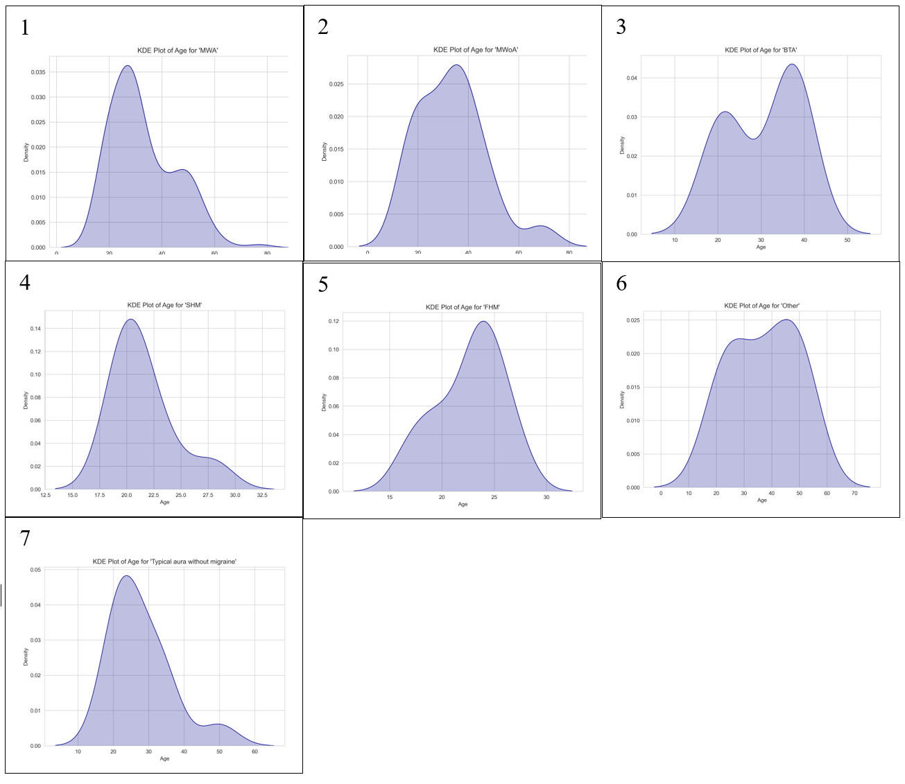
Figures A1, A2, A4, and A7 are all negatively skewed while Figures A3, A5, and A6 are all positively skewed. Similarly to the KDE plots generated for ‘Intensity’ they do not achieve normality. All 7 classes had enough variability for a KDE plot to be generated though which differed from Figure 2.
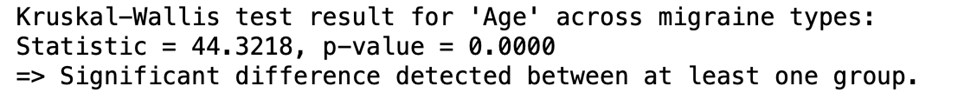
Figure B shows that between the seven migraine subtypes a p-value of 0.00 was determined. At a p-value of 0.00, there was a significant difference detected showing that there were differences between the 7 migraine classes when attributes were assessed among the patients.
| Group 1 | Group 2 | P-value | Significant |
| Basilar-type aura | Familial hemiplegic migraine | 1.65880761031109E-02 | TRUE |
| Basilar-type aura | Migraine without aura | 1E+00 | FALSE |
| Basilar-type aura | Other | 1E+00 | FALSE |
| Basilar-type aura | Sporadic hemiplegic migraine | 7.04463189342689E-02 | FALSE |
| Basilar-type aura | Typical aura with migraine | 1E+00 | FALSE |
| Basilar-type aura | Typical aura without migraine | 1E+00 | FALSE |
| Familial hemiplegic migraine | Migraine without aura | 4.10734449465188E-04 | TRUE |
| Familial hemiplegic migraine | Other | 1.0009361220668E-04 | TRUE |
| Familial hemiplegic migraine | Sporadic hemiplegic migraine | 1E+00 | FALSE |
| Familial hemiplegic migraine | Typical aura with migraine | 2.33574644024817E-05 | TRUE |
| Familial hemiplegic migraine | Typical aura without migraine | 1E+00 | FALSE |
| Migraine without aura | Other | 1E+00 | FALSE |
| Migraine without aura | Sporadic hemiplegic migraine | 1.09181113299382E-02 | TRUE |
| Migraine without aura | Typical aura with migraine | 1E+00 | FALSE |
| Migraine without aura | Typical aura without migraine | 1E+00 | FALSE |
| Other | Sporadic hemiplegic migraine | 1.24936302519723E-03 | TRUE |
| Other | Typical aura with migraine | 1E+00 | FALSE |
| Other | Typical aura without migraine | 1.27143477765745E-01 | FALSE |
| Sporadic hemiplegic migraine | Typical aura with migraine | 3.2145466555288E-03 | TRUE |
| Sporadic hemiplegic migraine | Typical aura without migraine | 1E+00 | FALSE |
| Typical aura with migraine | Typical aura without migraine | 6.85802027133075E-01 | FALSE |
Table A shows the results of the groups have significant differences. The Dunn’s test revealed statistically significant results between familial hemiplegic migraine and many other types of migraines including basilar-type aura (p=1.66e-02), migraine without aura (p=4.11e-04), other (p=1.0e-04), and typical aura with migraine (2.34e-05). This suggests that familial hemiplegic migraine is clinically distinct compares to the other types of migraine.
Appendix B – Character
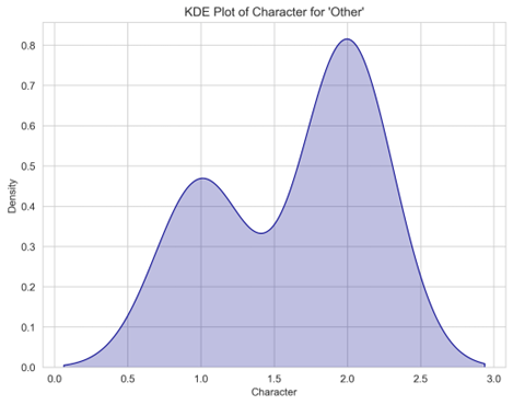
Figure C shows the only KDE plot generated for the attribute ‘Character.’ As with many other attributes, there was not enough variability to generate KDE plots of some types of migraine. The attribute character was one of the unique ones where only one KDE plot was generated.
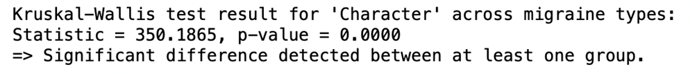
Figure D shows the Dunn’s test result for the attribute ‘Character’ across the seven migraine types. Since there was a significant difference between at least one pair of groups, it is suggested that ‘Character’ is clinically relevant in distinguishing migraine subtypes.
| Group 1 | Group 2 | P-value | Significant |
| Basilar-type aura | Familial hemiplegic migraine | 1E+00 | FALSE |
| Basilar-type aura | Migraine without aura | 1E+00 | FALSE |
| Basilar-type aura | Other | 2.45284478887769E-10 | TRUE |
| Basilar-type aura | Sporadic hemiplegic migraine | 1E+00 | FALSE |
| Basilar-type aura | Typical aura with migraine | 1E+00 | FALSE |
| Basilar-type aura | Typical aura without migraine | 1.16824996352733E-27 | TRUE |
| Familial hemiplegic migraine | Migraine without aura | 1E+00 | FALSE |
| Familial hemiplegic migraine | Other | 9.5788727680073E-12 | TRUE |
| Familial hemiplegic migraine | Sporadic hemiplegic migraine | 1E+00 | FALSE |
| Familial hemiplegic migraine | Typical aura with migraine | 1E+00 | FALSE |
| Familial hemiplegic migraine | Typical aura without migraine | 8.52147404084327E-32 | TRUE |
| Migraine without aura | Other | 1.42546799554599E-15 | TRUE |
| Migraine without aura | Sporadic hemiplegic migraine | 1E+00 | FALSE |
| Migraine without aura | Typical aura with migraine | 1E+00 | FALSE |
| Migraine without aura | Typical aura without migraine | 1.43782007064275E-43 | TRUE |
| Other | Sporadic hemiplegic migraine | 4.31141672528951E-09 | TRUE |
| Other | Typical aura with migraine | 1.19182305902666E-18 | TRUE |
| Other | Typical aura without migraine | 8.64238615372384E-71 | TRUE |
| Sporadic hemiplegic migraine | Typical aura with migraine | 1E+00 | FALSE |
| Sporadic hemiplegic migraine | Typical aura without migraine | 4.37118521371284E-24 | TRUE |
| Typical aura with migraine | Typical aura without migraine | 1.23986988690994E-53 | TRUE |
The Dunn’s test revealed statistically significant results between Other and many other types of migraines including typical aura with migraine. This suggests that familial hemiplegic migraine is clinically distinct compared to the other types of migraine
Appendix C- 45:55 test-train split
| Class | Precision | Recall | F1-score | Support |
| 0 | 0.88 | 0.95 | 0.91 | 111 |
| 1 | 0.84 | 1.00 | 0.92 | 27 |
| 2 | 0.83 | 0.62 | 0.71 | 8 |
| 3 | 0.75 | 0.50 | 0.60 | 6 |
| 4 | 0.33 | 0.18 | 0.24 | 11 |
| 5 | 1.00 | 0.25 | 0.40 | 8 |
| 6 | 1.00 | 1.00 | 1.00 | 9 |
| Accuracy | 0.86 | 180 | ||
| Macro avg | 0.81 | 0.64 | 0.68 | 180 |
| Weighted avg | 0.84 | 0.86 | 0.83 | 180 |
The RF model for the test-train split of 45:55 shows that there was insufficiency in predicting migraines in classes 2-5 as F1-scores were below 80% for each of them. Although the overall accuracy of the model was 86%, it is important to also take into consideration the macro average of the recall as 64% meaning that the machine learning model was not sufficient in predicting correct cases.
| Class | Precision | Recall | F1-score | Support |
| 0 | 0.89 | 1.00 | 0.94 | 111 |
| 1 | 0.96 | 1.00 | 0.98 | 27 |
| 2 | 1.00 | 0.62 | 0.77 | 8 |
| 3 | 1.00 | 0.17 | 0.29 | 6 |
| 4 | 0.60 | 0.55 | 0.57 | 11 |
| 5 | 1.00 | 0.25 | 0.40 | 8 |
| 6 | 1.00 | 1.00 | 1.00 | 9 |
| Accuracy | 0.89 | 180 | ||
| Macro avg | 0.92 | 0.66 | 0.71 | 180 |
| Weighted avg | 0.90 | 0.89 | 0.87 | 180 |
The ANN model for the test-train split of 45:55 shows that there was insufficiency in predicting migraines in classes 3-5 as F1-scores were significantly below 80% for each of them. Although the overall accuracy of the model was 89%, The recalls for classes 2-5 were all tremendously below 80% showing that the machine was insufficient in predicting correct cases.


Figure E gives a more detailed look into the TP, TN, FP, and FN of each machine learning model. For example, Figure E1 shows that the ANN model mostly misclassified patients in class 3 as patients in class 0. Figure E2 also shows that there was a there was a 50/50 accuracy on the machine’s predictions of patients in class 3. These are results that are highlighted in the classification reports in Tables C and D.
Appendix D- 75:35 test-train split
| Class | Precision | Recall | F1-score | Support |
| 0 | 0.86 | 0.98 | 0.92 | 185 |
| 1 | 0.94 | 1.00 | 0.97 | 45 |
| 2 | 0.86 | 0.43 | 0.57 | 14 |
| 3 | 0.33 | 0.10 | 0.15 | 10 |
| 4 | 0.36 | 0.22 | 0.28 | 18 |
| 5 | 1.00 | 0.38 | 0.56 | 13 |
| 6 | 1.00 | 1.00 | 1.00 | 15 |
| Accuracy | 0.86 | 300 | ||
| Macro avg | 0.76 | 0.59 | 0.63 | 300 |
| Weighted avg | 0.84 | 0.86 | 0.83 | 300 |
The RF model for the test-train split of 75:35 also shows that there was insufficiency in predicting migraines in classes 2-5 as F1-scores were below 80% for each of them. Although the overall accuracy of the model was 86%, the macro average of the recall as 59% meaning that the machine learning model was not sufficient in predicting correct cases. The recalls for classes 2-5 were also all significantly below 80%, especially class 3 at 10%.
| Class | Precision | Recall | F1-score | Support |
| 0 | 0.62 | 1.00 | 0.76 | 185 |
| 1 | 0.00 | 0.00 | 0.00 | 45 |
| 2 | 0.00 | 0.00 | 0.00 | 14 |
| 3 | 0.00 | 0.00 | 0.00 | 10 |
| 4 | 0.00 | 0.00 | 0.00 | 18 |
| 5 | 0.00 | 0.00 | 0.00 | 13 |
| 6 | 0.00 | 0.00 | 0.00 | 15 |
| Accuracy | 0.62 | 300 | ||
| Macro avg | 0.09 | 0.14 | 0.11 | 300 |
| Weighted avg | 0.38 | 0.62 | 0.47 | 300 |
Like Table 9, the ANN model was insufficient at predicting types of migraine apart from class 0 (recall=100%). Also, like Table F, the model incorrectly classified all the other patients as ones in class 0.

Figure F gives a more detailed look into the TP, TN, FP, and FN of each machine learning model. For example, Figure F1 shows that the ANN model was able to classify all 185 patients in class 0 correctly but also predicted all subsequent classes as class 0. Figure F2 shows more variation in comparison to F1. For example, all the patients in class 1 were correctly identified.
References
- T. J. Mungoven, L. A. Henderson and N. Meylakh, “Chronic Migraine Pathophysiology and Treatment: A Review of Current Perspectives,” Frontiers in Pain and Research, 2021. [↩] [↩]
- “Migraines,” 12 October 2022. [Online]. Available: https://www.hopkinsmedicine.org/health/conditions-and-diseases/headache/migraine-headaches. [Accessed 29 June 2025]. [↩]
- “Migraine,” [Online]. Available: https://www.ninds.nih.gov/health-information/disorders/migraine?search-term=migrain. [Accessed 13 June 2025]. [↩] [↩] [↩]
- I. Bonemazzi, F. Brunello, J. N. Pin, M. Pecoraro, S. Sartori, M. Nosadini and I. Toldo, “Hemiplegic Migraine in Children and Adolescents,” Journal of Clinical Medicine, vol. 12, no. 11, p. 3783, 31 May 2023. [↩] [↩] [↩] [↩]
- “Migraine Dataset,” 4 September 2023. [Online]. Available: https://www.kaggle.com/datasets/ranzeet013/migraine-dataset. [Accessed 2 January 2025]. [↩] [↩]
- “Glossary of Neurological Terms,” [Online]. Available: https://www.ninds.nih.gov/health-information/disorders/glossary-neurological-terms. [Accessed 18 July 2025]. [↩] [↩]
- A. P. Parate, A. A. Iyer, K. Gupta, H. Porwal and K. P.C., “Review of Data Bias in Healthcare Applications,” International Journal of Online and Biomedical Engineering, 13 September 2024. [↩] [↩]
- “The Basics of Migraine with Brainstem Aura,” 8 October 2016. [Online]. Available: https://americanmigrainefoundation.org/resource-library/migraine-with-brainstem-aura/. [Accessed January 2025]. [↩]
- J. R. Kim, T. J. Park, M. Agapova, A. Blumenfeld, J. H. Smith, D. Shah and B. Devine, “Healthcare resource use and costs associated with the misdiagnosis of migraine,” Headache, vol. 65, no. 1, pp. 35–44, 28 August 2024. [↩]
- “Familial Hemiplegic Migraine,” 4 July 2024. [Online]. Available: https://www.ncbi.nlm.nih.gov/books/NBK1388/. [Accessed 28 June 2025]. [↩]
- L. Khan, M. Shahreen, A. Qazi, S. J. A. Shah, S. Hussain and H.-T. Chang, “Migraine headache (MH) classification using machine learning methods with data augmentation,” Scientific Reports, vol. 14, no. 1, 2 March 2024. [↩]
- A. Reddy and A. Reddy, “Migraine Triggers, Phases, and Classification using Machine Learning models,” Frontiers in Neurology, vol. 16, 8 May 2025. [↩]
- R. d. Filippis and A. A. Foysal, “The Impact of Machine Learning in Identifying Migraine Types: A Data-Driven Approach,” OALib, vol. 12, no. 4, pp. 1–17, 2025. [↩]
- J. Rogers and A. Jonker, “What is data bias?,” 4 October 2024. [Online]. Available: https://www.ibm.com/think/topics/data-bias. [Accessed 28 June 2025]. [↩]
- J. Starmer, “StatQuest: Random Forests Part 1 – Building, Using and Evaluating [Video],” 5 February 2018. [Online]. Available: https://www.youtube.com/watch?v=J4Wdy0Wc_xQ. [Accessed January 2025]. [↩] [↩]
- J. Starmer, “StatQuest: Decision and Classification Trees, Clearly Explained!!! [Video],” 26 April 2021. [Online]. Available: https://www.youtube.com/watch?v=_L39rN6gz7Y. [Accessed January 2025]. [↩] [↩]
- G. Sebastianelli, D. Secci, F. Casillo, C. Abagnale, C. D. Lorenzo, M. Serrao, S.-J. Wang, F.-J. Hsiao and G. Coppola, “Artificial Neural Networks Applied to Somatosensory Evoked Potentials for Migraine Classification,” The Journal of Headache and Pain, vol. 26, no. 1, 4 April 2024. [↩]
- N. Acharya, “Understanding Precision, Recall, F1-score, and Support in Machine Learning Evaluation,” 15 February 2024. [Online]. Available: https://medium.com/@nirajan.acharya777/understanding-precision-recall-f1-score-and-support-in-machine-learning-evaluation-7ec935e8512e. [Accessed 17 February 2025]. [↩]
- “Understanding the Confusion Matrix in Machine Learning,” 30 May 2025. [Online]. Available: https://www.geeksforgeeks.org/machine-learning/confusion-matrix-machine-learning/. [Accessed 16 February 2025]. [↩]
- “What is ANOVA (Analysis of Variance),” 19 July 2023. [Online]. Available: https://www.editage.com/blog/anova-types-uses-assumptions-a-quick-guide-for-biomedical-researchers/. [Accessed 18 July 2025]. [↩] [↩] [↩] [↩] [↩] [↩] [↩]
- R. Bevans, “One-way ANOVA | When and How to Use It (With Examples),” 10 May 2024. [Online]. Available: https://www.scribbr.com/statistics/one-way-anova/. [Accessed 28 June 2025]. [↩] [↩] [↩] [↩] [↩]
- S. Lomuscio, “Getting Started with the Kruskal–Wallis Test,” 7 December 2021. [Online]. Available: https://library.virginia.edu/data/articles/getting-started-with-the-kruskal-wallis-test. [Accessed 14 July 2025]. [↩]
- T. J. Cleophas and A. H. Zwinderman, “Non-parametric Tests for Three or More Samples (Friedman and Kruskal–Wallis),” Clinical Data Analysis on a Pocket Calculator, pp. 193–197, January 2016. [↩] [↩]
- S. Biswas, N. Grundlingh, J. Boardman, J. White and L. Le, “A Target Permutation Test for Statistical Significance of Feature Importance in Differentiable Models,” Electronics, vol. 14, no. 3, p. 571, 31 January 2025. [↩] [↩] [↩]


