
Abstract
This research develops a reinforcement learning (RL)-based neural network (NN) to optimize orbital transfers in low Earth orbit. Traditional methods, such as the Monte Carlo (MC) simulation, require numerous computational resources and iterations; the proposed RL is benchmarked by the MC and produces more accurate results across all metrics, past a threshold of training. With further development reducing necessary on-board computations, the proposed RL has potential viability to replace MC for satellite servicing missions. The RL was trained on four Hohmann and non-coplanar transfer scenarios, and the results demonstrate progression in the NN’s accuracy given more timesteps. The results indicate RL’s capability to predict optimal trajectories and adapt to varying scenarios, offering potential reductions in cost and computation for future satellite servicers. This proof of concept establishes the foundation for RL-based NN applications in more complex orbital mechanics problems, specifically real-time scenarios with live trajectory updates.
Keywords: Machine learning, reinforcement learning, orbital mechanics, low Earth orbit, orbital transfer, Hohmann transfer, neural networks
Introduction
Background and Context
There is an increasing necessity for satellite maintenance. With the countless developments in satellite maintenance technology, there is a strong demand to update them to enhance performance. Disposing of and replacing the 12,000 satellites orbiting Earth is neither fiscally nor environmentally advantageous. One of the popular solutions to this issue is the creation of servicing satellites, which would intercept and update old satellites without disrupting their orbits.
The foundation of this manuscript, the four orbital-transfer scenarios, is grounded in orbital mechanics, with an analytic optimum benchmarking the simulations’ performance1. Curtis summarizes how Hohmann and non-coplanar transfers provide exact solutions for impulses and durations of flight, which makes these transfers ideal examples employed for evaluation.
Raychaudhuri2 describes Monte Carlo (MC) simulation as a widely used, fundamental approach for simulation-based analysis that relies on repeated random sampling, requiring trials in the thousands to stabilize results. However, the MC approach is limited by its linear scaling and cost of each propagation. Peherstorfer3 states that uncertainty propagation in aerospace is often based on the MC simulation, but becomes exceptionally expensive and “computationally intractable” when used in high-fidelity models.
Even with analytic optimums derived from Curtis1, realistic, real-time missions typically involve no closed form Hohmann solution. MC simulations, as summarized by Raychaudhuri2 and Peherstorfer3, require many propagations that become costly in high-fidelity dynamics. Reinforcement Learning (RL) is a potential solution to reduce these costs. RL is a framework where an AI agent interacts with an environment, improving through a reward-based, trial-and-error policy4‘5. Recent research increasingly utilizes RL to solve astrodynamics problems, including trajectory optimization, multi-body guidance, and rendezvous6‘4‘7‘8‘9‘10‘11‘12‘13.
Problem Statement and Rationale
While reinforcement learning has been applied to low-thrust or multi-body trajectory problems, there is limited evidence that RL has been compared with MC performance for canonical impulsive orbital transfers with analytically known optima.
Impulsive orbital transfers are fundamental tools for spacecraft maneuvering, particularly for charting the optimal trajectories for satellite servicers. Because these transfers are often high-cost and time-sensitive, missions benefit from swift estimation methods. Classical analytical methods, such as those derived from Curtis1, produce exact maneuvers in idealized conditions. However, real-time missions rarely imitate a perfect environment, and high-fidelity models require expensive propagations, making the MC simulation a costly method3. Therefore, the approach for impulsive orbital transfers is subject for improvement with more computationally efficient algorithms.
Prior research demonstrates how RL can be applied to astrodynamics problems ranging from low, continuous thrust; to multi-body dynamics; to guidance and angles-only rendezvous14‘7‘8‘15‘13. However, these works are not compared to an analytic optimum, which is a natural limitation of working with problems with no closed form solutions. Kolosa4, for instance, demonstrates that deep RL can optimize continuous low-thrust trajectories for multiple mission types. However, like many other RL-based astrodynamics studies, it does not address impulsive, two-body transfers, nor does it examine performance across several Lower Earth Orbit (LEO) scenarios against a MC baseline. These studies offer valuable insights into RL’s capabilities, but they remain untested against a true optimum and unbenchmarked by a traditional MC simulation.
This gap serves as the motivation for the present paper. By focusing on transfers with analytically known optima, we can comprehensively evaluate the RL’s progress across multiple scenarios. Benchmarking the RL’s performance with the MC’s under matched conditions allows for direct comparison, demonstrating an RL’s potential viability to replace MC for satellite servicing missions.
Significance and Purpose
The number of active satellites is exponentially increasing, with replacement extremely costly. Thus, there is an emerging demand for satellite servicers: robots that intercept satellites in orbit and provide maintenance or improvements. Traditional approaches like the MC sim are computationally heavy and unideal for high-fidelity rapid, real-time propagation updates.
This study showcases the potential for an RL method to be a solution, offering a controlled benchmark to an analytic optimum and MC simulation for a trained RL policy. With expansion and more training, theoretically an RL policy has the potential to make more rapid maneuvers with few episodes. Therefore, theoretically, onboard computation costs and times could be reduced if a more developed RL model is implemented on a satellite servicer.
Moreover, the true optimality gap offers an opportunity to better analyze how an RL performs in a deterministic, analytic environment. This study could benefit researchers studying machine learning alternatives to control problems in the field of aerospace and astrodynamics.
Objectives
The objective is to create a RL-based Neural Network (NN) that generates the most cost-efficient orbital transfers for an appropriate rendezvous location, respective to the servicer’s initial location and the orbital path of the target satellite. This research demonstrates if there is a potential for RL to reduce onboard computations for satellite servicers. In addition, the RL will be directly compared with a MC simulation, where actions and environments are matched in Hohmann and non-coplanar transfer scenarios. The results of both simulations will be evaluated on each scenario’s pre-calculated, idealized actions and target rendezvous locations. The result will be an assessment that demonstrates if RL has the potential to become a more efficient method than MC in more complex orbital mechanics problems, specifically real-time scenarios with live trajectory updates.
Scope and Limitations
This study focuses on two-body impulsive transfers in LEO, ranging from canonical Hohmann transfers to co-planar, multi-transfer missions. The RL and MC are evaluated on four transfer scenarios with varying starting and target coordinates and velocities. For each scenario, the RL and MC are equipped with the same action space and environment. Evaluation metrics include average, median, and best position and  V errors, including acceptance thresholds for both simulations.
The environment for the simulations is kept simple, neglecting perturbations such as LEO drag, J2, or third-body gravity influence. Additionally, the scenarios’ environments do not include the natural noise in state estimation and V measurements that exist in real-world scenarios. The present simulations allow for zero uncertainty, which has only been tested in environments with ideal physics.
Theoretical Framework
Three theoretical frameworks are combined to produce this paper: Markov Decision Processes (MDP), two-body orbital mechanics, and benchmarking. Firstly, the developed RL contains the MDP framework, which is defined as a process where an AI agent makes an action in an environment that results in a state which the agent receives feedback on16. This cycle mirrors the process of the RL, where the LEO setting, initial coordinates and starting velocities represent the environment; the impulse(s) the servicer may take relate to the MDP action space; and the analytic gap between the final state and the target position serve as a reward equation– feedback for the agent. This MDP framework is a means to conceptualize the RL policy’s training process, which is integral to its potential as a method for calculating transfers. Secondly, the analytic optimum is derived from the two-body dynamics of Hohmann and non-coplanar transfers. This framework is rooted in orbital mechanics, which is the study of the motion of artificial satellites under gravity, thrusts, drag, and other perturbations1. The idealized burns calculated from this framework are essential tools for evaluation, specifically in producing the optimality gap for V. Lastly, the comparison between the RL and MC simulations is applied through a benchmarking framework, which is a method of establishing a standard– the MC– as a means to evaluate performance of a new method under review. This framework is vital, as it allows for direct comparison between the traditional and experimental simulations.

Methodology Overview
Four orbital transfer scenarios are created, with varying starting and target coordinates. With initial and target states selected, the ideal burns and burn locations (for muli-burn transfers) are calculated with standard orbital mechanics equations. These analytic optimums are used to evaluate the RL and MC performance.
A deterministic two-body environment is implemented for each scenario using the Poliastro libraries to propagate states and ensure the LEO dynamics17. The RL agent is trained in each scenario with a bounded  action space. The agent only receives feedback on each episode’s analytic gap for its final position, being penalized for bigger gaps. Following the MDP framework, errors are not used in training. Each final model for the scenarios is saved for evaluation.
A MC simulation, given the same bounded action space, is run for 5000 trials in each scenario’s environment. Every scenario’s trained RL policy is run for 5000 rollouts under the same conditions. Ran Monte Carlo sim using exact same parameters as the RL’s for each scenario to allow for direct performance comparison.
Methods
Research Design
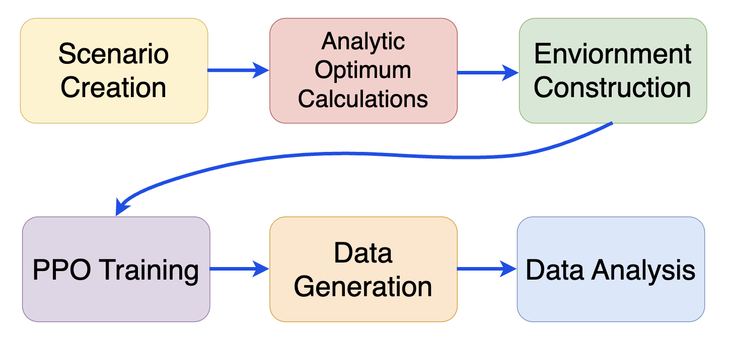
This numerical experiment produces a deterministic two-body orbital mechanics simulation based on Poliastro dynamics17 and utilizes comparative evaluation between RL and MC algorithms. Four orbital transfer scenarios are tested; one through three reflect that of a canonical Hohmann transfer, and scenario four involves multiple burns and a plane change maneuver. The developed RL models’ and MC’s performances are evaluated on analytic optima derived from foundational orbital mechanics equations1. The RL agent is trained with Proximal Policy Optimization (PPO) and Multilayer Perceptron (MLP) architecture. PPO uses a policy-gradient method, actor-critic architecture, and a clipping mechanism to maximize results without diverging too far from the model’s past states18. The process is as follows: set up (scenario creation, idealized burn calculations), RL training and rollouts, MC trials, evaluation through comparison.

Analytic Optimum Calculations
Every scenario is calculated using the orbital mechanics found in Curtis’s textbook1. The following formulas are used to derive the analytic optima for RL and MC evaluation.
The semi-major axis indicates the size of an elliptical orbit: is the orbit’s radius of apoapsis and is an orbit’s radius of periapsis.
(1) 
Vis-Viva:  is the orbital velocity,
  is the universal gravitational constant, and
  is the orbital radius, and
  is the semi-major axis.
(2) 
Orbital velocity for a circular orbit (derived from Vis-Viva)
(3) 
Orbital velocity for non-circular orbits
(4) 
Orbital eccentricity, which affects the shape of the orbital path: variable  is the orbit’s eccentricity,
  is the orbit’s radius of apoapsis,
  is an orbit’s radius of periapsis.
(5) 
Specific angular momentum of an orbit, or the product of an object’s rotational inertia and the angular velocity divided by its mass:  represents the angular momentum.
(6) 
Total delta-v represents the summation of all the changes in the orbital velocity necessary to complete the transfer.  represents the change in velocity at periapsis and
  represents the change in velocity at apoapsis.
(7) 
Period of transfer:  represents the time in seconds for a transfer to occur.
(8) 
Combined plane-change for one impulse:  represents the angle of the plane change.
(9) 
Scenario One
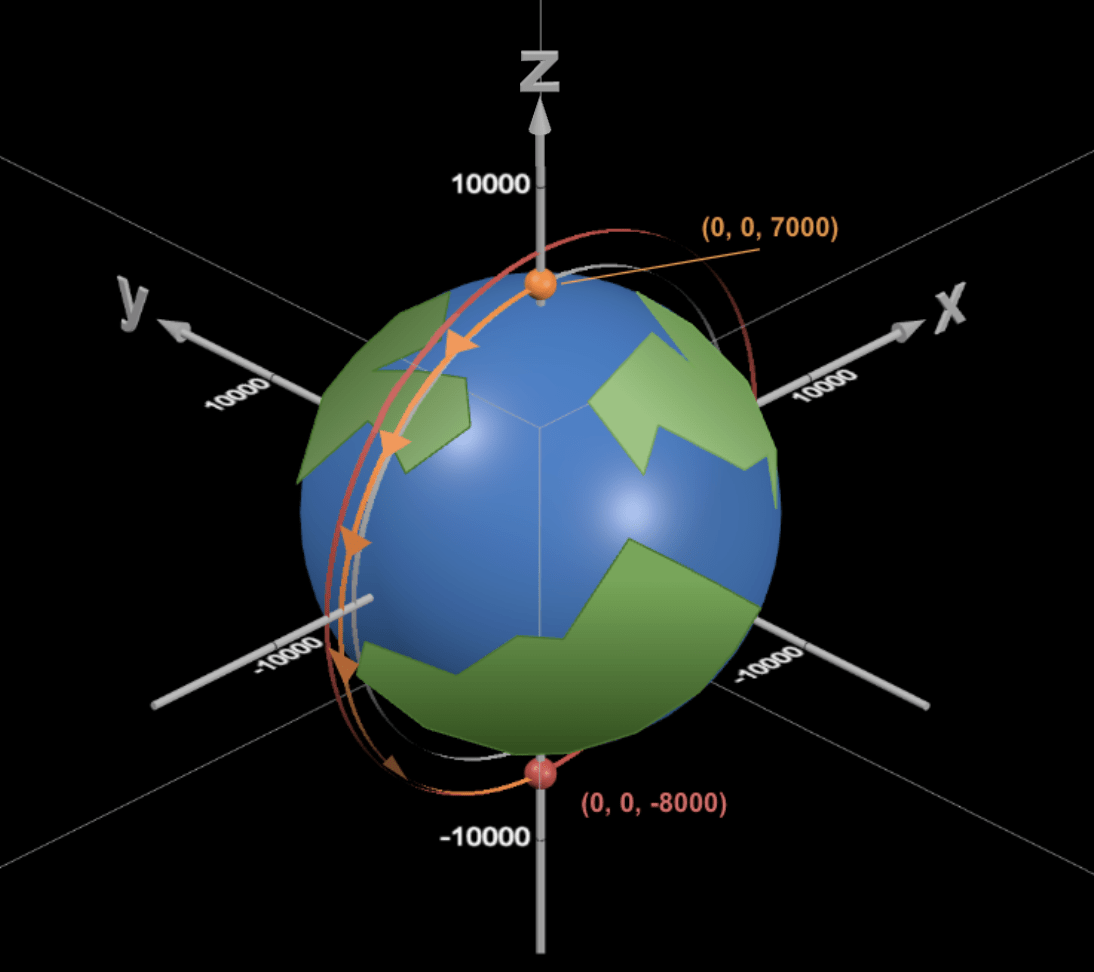
The starting coordinates for scenario one are (0, 0, 7000) in kilometers, with an initial velocity of (-7.54607, 0, 0) in kilometers per second. The target coordinates are (0, 0, -8000), and the ideal impulse is 0.247477 kilometers per second. The expected time of flight is 3232.013 seconds.
Scenario two
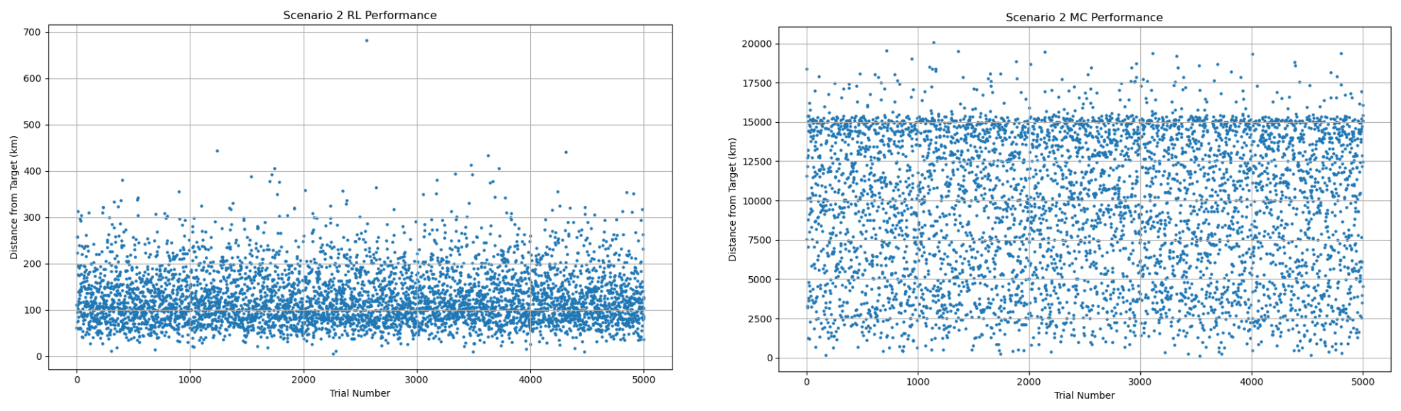
The starting coordinates for scenario two are (0, 0, 6900) in kilometers, with an initial velocity of (-7.58948, 0, 0), which is slightly eccentric, in kilometers per second. The target coordinates are (0, 0, -8200), and the ideal impulse is 0.320421188 kilometers per second. The expected time of flight is 3264.387 seconds.
Scenario Three
The starting coordinates for scenario three are (0, 0, 7400) in kilometers, with an initial velocity of (-7.33927, 0, 0) in kilometers per second. The target coordinates are (0, 0, -8200), and the ideal transfer is 0.185833679 kilometers per second. The expected time of flight is 3427.860 seconds.
Scenario Four
The starting coordinates for scenario four are (-7100, 0, 0) in kilometers, with an initial velocity of (0, 7.49272, 0) in kilometers per second. The ideal initial impulse is -0.24255 kilometers per second; the ideal coordinates for the second burn are (8100, 0, 0), with the ideal second impulse being 1.22486 kilometers per second, which can be broken into (0, 0.12811, 1.21814); and the final target coordinates are  . The expected time of flight is 5110.624 seconds.
Simulation Environment and Data Generation
A two-body point mass Earth model is implemented for the environmental physics, with ( ) representing the gravitational parameter. Poliastro handled all propagation17. Perturbations, such as
  , drag, and additional third-body gravity, are neglected. Distances are measured in kilometers, and time is measured in seconds. There is no uncertainty or noise in the environment, with deterministic outcomes for every action. The environment is given an initial position and velocity vector, and the output is a final position and velocity vector.
For two-impulse scenarios, a leg-index flag has been implemented to distinguish impulses. The two-impulse scenario outputs four variables: mid-state position, mid-state velocity, final position, and final velocity vectors. The RL agent receives no feedback on errors or time of flight for any scenario. Each trial is truncated once the analytic time of flight has been reached.
For Hohmann transfers, the action space is a three-dimensional vector that represents the instantaneous impulse:  . Non-coplanar transfers have seven actions: two three-dimensional vectors and the time to apply the second burn. The orbits are propagated deterministically– after applying the instantaneous impulse, the RL outputs the final coordinates. Each episode is a MDP.
For every scenario after training, the RL produces 5000 samples using its final model. The MC baseline generates 5000 samples from the same environment, action space, and propagation pipeline. Therefore, each scenario has 5000 RL and MC samples, which is 40000 generated samples across all experiments in total. The number of MC samples is chosen to ensure stable distributions and statistical significance. The RL produces the same number of samples to acknowledge the PPO’s stochastic variation and maintain impartial comparison between the two simulations.
Variables and Measurements
The observation space of the RL expresses a scenario’s position  in kilometers and velocity
  in kilometers per second. State variables follow those of Poliastro’s, which is km and km/s. The variables for position, time, velocity, and for the analytic optimum are kilometers, seconds, kilometers per second, and kilometers per second, respectively.
Action variables for a Hohmann transfer scenario are an impulse of in kilometers per second. If the scenario involves multiple impulses, the RL’s actions include the ideal number of impulses in kilometers per second and the time (in seconds) of flight to perform the additional impulse.
The reward is structured as a negative position error between the analytic optimum and each trial’s final position. For the RL to discover the optimal maneuvers, the analytic optimum for is not included in the reward equation; this simulates real-world missions, which will only have the coordinates of the satellite and not a pre-calculated ideal burn for the RL to copy. Thus, the RL employs an unsupervised learning model. The reward is therefore measured in kilometers.
(10) 
Procedure
Step One: Scenario definition and Analytic Optima Calculations
Initial and target circular LEO orbits are defined in a configuration file. Scenarios one through three are single impulse, Hohmann transfers, and scenario four is a multi-impulse, non-coplanar transfer.
Using orbital mechanics principles and formulas1 analytic optima are calculated before training. Specifically, the ideal impulses are derived and stored for later evaluation, and ideal times of flight are used to truncate the algorithms’ trials. The time of fight and ideal position for the second burn of the two-impulse case are also calculated.
Step Two: Environment Construction
The simulations’ environment, titled OrbitalTransferEnv, has a state representation of position and velocity vectors in Cartesian coordinates. The two-impulse scenario’s environment tracks the number of impulses and the time of flight along both transfers.
Gravitational parameters and the LEO two-body point mass model are consistent across scenarios17, and truncation is fixed on the ideal time of flight, respective to each scenario’s analytic solution. The environment is constructed for an unsupervised training regime, so it only contains the target positions and does not interact with the ideal .
For scenarios one through three, their action spaces consisted of a three-dimensional vector that is applied at its initial state. For scenario four, its action space consisted of two three-dimensional vectors and a time of flight for when to apply the second burn.
All actions are bounded by 2 kilometers per second, which is a range suitable for cost-efficient LEO transfers and comfortably contains the analytic solutions for every scenario.
Deterministic propagations for selected impulse(s) result in immediate final positions, which are then fed to the reward equation [equation 10] that computes the final position error from the analytic solution. This terminal position error is then normalized by  (the larger of the two orbital radii in the present scenario), for stability and to ensure reasonable comparison across scenarios. This reward returns a negative and represents one step in the MDP.
Step Three: PPO Training
Stable Baseline Three is used for its built-in PPO and MLP policies18‘19. PPO updates the NN after collecting 2,048 state transitions per update. The MLP policy is the NN’s architecture, with two hidden layers, 64 activation units with tanh activations. The main hyperparameters are as follows: the learning rate is 3 10
10 , which is magnitude of NN updates between batches; the batch size is 64, which is the number training examples before a minor update;
  is 0.99, which represents the emphasis on future rewards;
  is 0.95, which compares estimated and actual rewards; and the clip range is 0.2, which prevents drastic updates to the NN.

The training lasted 500,000 timesteps for scenarios one and two, 1,000,000 for scenario three, and 1,200,000 for scenario four. Scenario four is given more timesteps because it is a two-impulse transfer, with
more than double the number of variables in its action space. Scenario three, with the same general structure as transfers one and two, has more timesteps for a sensitivity check. For every scenario, after 50,000 timesteps had passed, the training would pause and run an evaluation on the past 50 episodes to log the mean position and errors. These progress checks are saved in a progress_eval.csv file; and, once training is completed, the model gets saved as a final_model.zip for every scenario.
Step Four: Generating Data for RL and MC
To evaluate the trained RL, the model is run stochastically over 5,000 samples for each scenario and saved into a CSV file. Each sample runs with the same MLP, logging its actions and returning its terminal position and errors.
The MC, using the same action space and environment as the RL, runs over 5,000 samples, generating random actions and drawing identical categories of variables as the RL. These records are stored in a MC-specific CSV file.
Data Analysis
The terminal position and errors are the Euclidean norm between the final and analytical optimums. It is important to note: while the terminal error for the action space is used in evaluation, the total velocity error–the difference between the final and target velocities– is not
The total terminal velocity error evades evaluation because neither simulation has the agency in its action spaces to course-correct to the target orbital velocity. Therefore, it would be unrealistic to see the RL or MC’s terminal velocity mirror the analytical terminal velocity. The goals of these simulations are target position interception and cost-optimization of the impulses they control.
The mean, median, and best (smallest) of the errors for position and are then calculated, with pass-rate metrics of position equal to or under fifty kilometers and velocity equal to or under 0.2 kilometers per second.
The performance of MC and RL simulations is evaluated under identical conditions, with an equal number of 5,000 samples for fair comparison. All samples from each scenario are stored in CSV files, and Python scripts extract the data to produce the aforementioned metrics into summary tables and scatter plot distributions using Pandas and MatPlotLib.
Due to their continuous and skewed nature, Mann-Witney U tests are done to evaluate the RL and MC error distributions; and due to their binary nature, two proportion z–tests are done to compare the pass-rates of the two simulations.
The results are interpreted by how closely the terminal position and match the analytical solutions, or how closely their errors approach zero. MC represents an untrained version of sampling, benchmarking the RL’s unsupervised training. The varying scenarios and timesteps allow for a more comprehensive interpretation of how these variables affect RL and MC performance.
Ethical Considerations
All data in this study are collected through simulation and did not draw from any preexisting datasets.
This research is conducted with regard to transparency and reproducibility.
Results
Scenario One
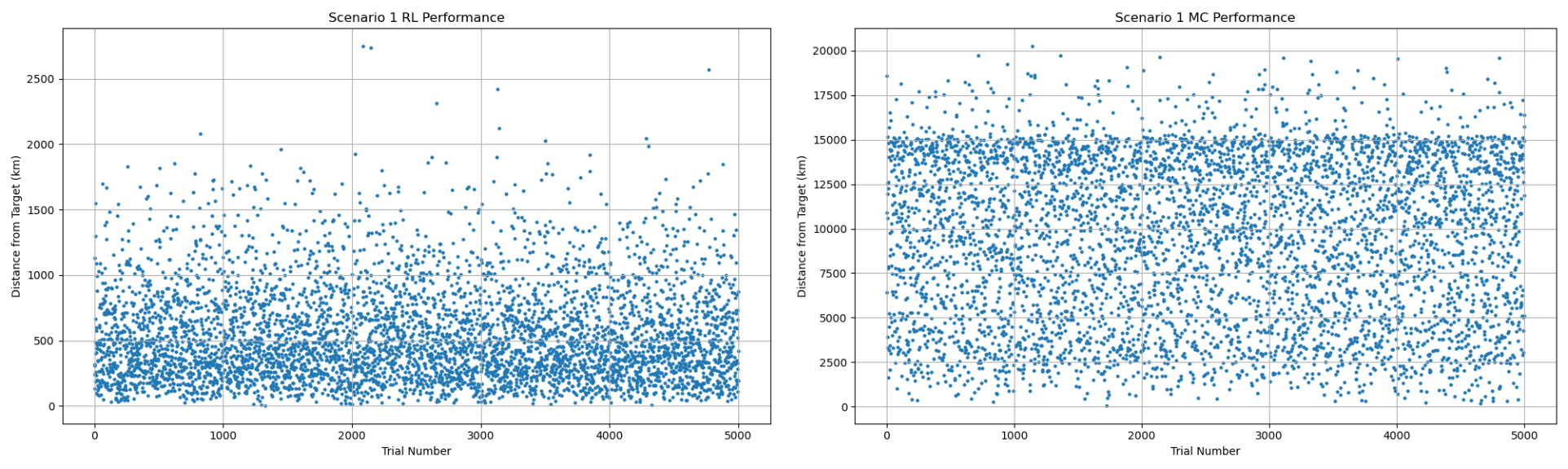
RL Performance (5000 samples) MC Performance (5000 samples)
| Metric | RL | MC |
| Sample size | 5,000 | 5,000 |
| Timesteps | 500,000 | N/A |
| Position error mean (km) | 539.36 | 9,452.36 |
| Position error median (km) | 453.51 | 9958.28 |
| Position error best (km) | 3.40 | 66.35 |
| error mean (%) | 112.52 | 675.36 |
| error median (%) | 80.60 | 696.34 |
| error best (%) | 0.03 | 0.03 |
Position pass rate (  50 km) (%) 50 km) (%) | 1.12 | 0.00 |
| pass rate ( 20 m/s) (%) | 5.52 | 0.02 |
| Metric | RL | MC |
| Sample size | 5,000 | 5,000 |
| Timesteps | 500,000 | N/A |
| Position error mean (km) | 126.45 | 9,602.09 |
| Position error median (km) | 112.88 | 10,142.97 |
| Position error best (km) | 5.66 | 125.90 |
| error mean (%) | 20.18 | 498.91 |
| error median (%) | 9.72 | 515.05 |
| error best (%) | 0.00 | 0.37 |
| Position pass rate ( 50km) (%) | 4.12 | 0.00 |
| pass rate (20 m/s) (%) | 41.36 | 0.02 |
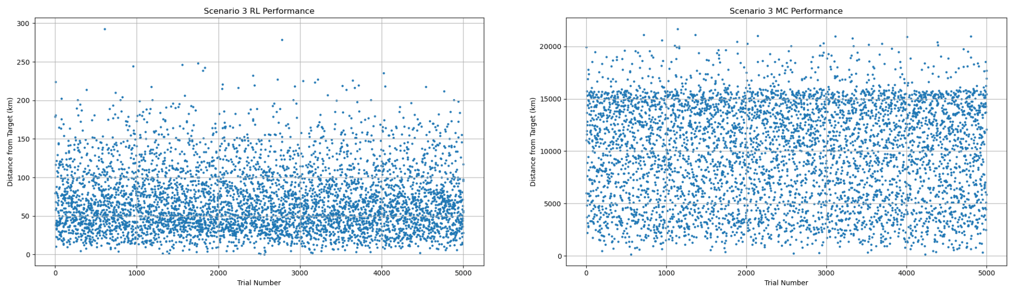
| Metric | RL | MC |
| Sample size | 5,000 | 5,000 |
| Timesteps | 1,000,000 | N/A |
| Position error mean (km) | 70.10 | 9,908.57 |
| Position error median (km) | 60.93 | 10,463.68 |
| Position error best (km) | 0.46 | 161.16 |
| error mean (%) | 29.80 | 932.49 |
| error median (%) | 18.22 | 960.50 |
| error best (%) | 0.00 | 0.395 |
| Position pass rate ( 50 km) (%) | 38.50 | 0.00 |
| pass rate ( 20 m/s) (%) | 37.28 | 0.01 |
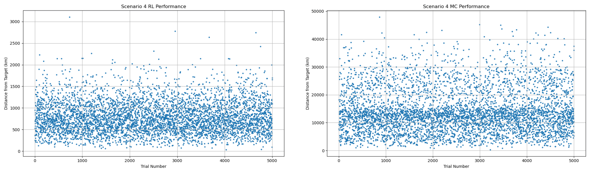
| Metric | RL | MC |
| Sample size | 5,000 | 5,000 |
| Timesteps | 1,200,000 | N/A |
| Position error mean (km) | 784.04 | 14,116.32 |
| Position error median (km) | 735.95 | 12,649.44 |
| Position error best (km) | 36.44 | 350.11 |
| error mean (%) | 18.05 | 161.15 |
| error median (%) | 15.62 | 163.32 |
| error best (%) | 0.01 | 0.13 |
| Position pass rate ( 50 km) (%) | 0.04 | 0.00 |
| pass rate ( 20 m/s) (%) | 4.78 | 0.00 |
Discussion
Restatement of Key Findings
The RL agent consistently outperformed the MC simulation across all four scenarios. The MC matches or outperforms the RL in only 3.125% of cases, and only occurs in scenarios with intentionally limited timesteps. In every instance, across all scenarios, the RL achieved a dramatically lower mean and median terminal position and The RL agent consistently outperformed the MC simulation across all four scenarios. The MC matches or outperforms the RL in only 3.125 % of cases, and only occurs in scenarios with intentionally limited timesteps. In every instance, across all scenarios, the RL achieved a dramatically lower mean and median terminal position and errors compared to MC. This is reflected in the Mann-Whitney U tests for velocity and position errors between RL and MC, with  values ranging from 85 to 87 and p-values effectively zero, indicating extreme differences in the simulations’ distributions. Scenarios with more timesteps (three and four) demonstrate a 99.97% to a 92% decrease, respectively, from MC to RL in best errors Scenario three produces the strongest results, with the RL achieving a 38.5% pass rate for the position error threshold, and 37.28% for Scenario three produces the strongest results, with the RL achieving a 38.5% pass rate for the position error threshold, and 37.28% for ‘s. In fact, Scenario three’s error is smaller than the MC’s more than 99.99% of the time. The MC rarely, if at all, achieves a pass rate above 0.02% for any metric. Across all scenarios, a two-proportion z-test for pass rate distributions was conducted With z-scores between 7.50 to 50.79 and
  , the RL’s outperformance for and position pass rate is statistically significant across all scenarios. However, while Scenario four’s RL’s position pass rate is ten times greater than the MC’s, its p-value of 0.157 and z-score of 1.41 does not imply significance, which can be attributed to the increased difficulty of the transfer. The RL displays a strong sensitivity to the number of timesteps for training, with a positive correlation between the timesteps and accuracy to the analytical optima; increasing the scenario’s difficulty has the opposite effect.
Implications and Significance
These findings show that RL has a clear potential to outperform MC simulations in on-board satellite servicing missions, producing significantly more accurate results when given adequate training experience. These results support the hypothesis that RL is viable to be a more computationally efficient alternative to the traditional MC in high-fidelity dynamics. Its ability to accurately estimate the ideal burn with only its current position, velocity, and rendezvous location demonstrates its potential to rapidly make orbital transfers in real-time missions. This study provides a MC benchmark with the RL performance, filling an existing research gap. The results strongly indicate that, with an investment in more training, RL could be an asset to the satellite servicing industry.
Connection to Objectives
An RL-based NN has been developed that generates the most cost-efficient orbital transfers based on a given rendezvous location. This research demonstrates the potential for RL to reduce onboard computations for satellite servicers. In addition, the RL has been directly compared with a MC simulation, where actions and environments are matched in Hohmann and non-coplanar transfer scenarios. Both simulations have been evaluated on every metric for every scenario. A comprehensive assessment has been produced that demonstrates RL’s potential as a more efficient method than MC in complex orbital mechanics problems, specifically real-time scenarios with live trajectory updates.
Recommendations
The results of this study strongly indicate a recommendation to expand and deepen RL training for a diverse set of orbital transfer scenarios. Introducing the aforementioned perturbations, such as LEO drag, J2, or third-body gravity influence, would be a significant step towards producing an RL fit for a servicer. Beyond satellite servicing, an RL could also be trained to account for and dodge obstacles, course-correcting by applying burns mid-transfer. Additionally, a performance comparison between different RL architectures (TRPO, SAC, GRPO, etc.) to optimize policy is recommended.
Limitations
The environment uses deterministic two-body propagation, neglecting perturbations such as LEO drag, J2, or third-body gravity influence. Additionally, the scenarios’ environments do not include the natural noise in state estimation and Δv measurements that exist in real-world scenarios. The present simulations allow for zero uncertainty, only tested in environments with ideal physics. Lastly, the training timesteps are kept limited (500k–1.2M); further training would likely improve RL performance.
Closing Thought
This study reveals that RL can estimate impulsive LEO orbital transfers and, beyond a certain training threshold, consistently outperforms the MC simulation. If this NN is further developed, the calculations for the paths and costs of satellite servicers would become significantly more affordable, leading to increased production and optimized schedules. This proof-of-concept demonstrates that RL may be a value asset to satellite servicers in the future.
Acknowledgements
All contents (scenario construction, analytical calculations, experiments, and writing) are the original work of the first and second authors. ChatGPT 5.1 and Grammarly are used only as coding, manuscript structuring, and grammar revision tools, guided, debugged, and modified by author input.
References
- H. D. Curtis. Orbital mechanics for engineering students. Elsevier Butterworth-Heinemann. Burlington, MA, 2005. [↩] [↩] [↩] [↩] [↩] [↩] [↩]
- S. Raychaudhuri. Introduction to Monte Carlo simulation. Winter Simulation Conference Proceedings, 2008. [↩] [↩]
- B. Peherstorfer, P. Beran, K. E. Willcox. Multifidelity Monte Carlo estimation for large-scale uncertainty propagation. AIAA Non-Deterministic Approaches Conference, 2018, https://dspace.mit.edu/handle/1721.1/114856. [↩] [↩] [↩]
- D. S. Kolosa. A Reinforcement Learning Approach to Spacecraft Trajectory Optimization. Ph.D. dissertation, Western Michigan University, 2019, https://scholarworks.wmich.edu/dissertations/3542/. [↩] [↩] [↩]
- D. Miller, R. Linares. Low-Thrust Optimal Control via Reinforcement Learning. ResearchGate. 2019, https://www.researchgate.net/publication/331135625. [↩]
- C. M. Casas, B. Carro, A. Sanchez-Esguevillas. Low-Thrust Orbital Transfer Using Dynamics-Agnostic Reinforcement Learning. arXiv preprint arXiv:2211.08272, 2022,https://arxiv.org/abs/2211.08272. [↩]
- N. LaFarge, D. Miller, K. C. Howell, R. Linares. Autonomous closed-loop guidance using reinforcement learning in a low-thrust, multi-body dynamical environment. Vol. 186 Acta Astronautica., 2021, https://doi.org/10.1016/j.actaastro.2021.05.014. [↩] [↩]
- D. Miller, R. Linares. Low-Thrust Optimal Control via Reinforcement Learning. ResearchGate, 2019, https://www.researchgate.net/publication/331135625. [↩] [↩]
- A. Zavoli, L. Federici. Reinforcement Learning for Robust Trajectory Design of Interplanetary Missions. Journal of Guidance, Control, and Dynamics, Vol. 44, no. 8, 2021, https://doi.org/10.2514/1.G005794. [↩]
- L. Federici, A. Zavoli, et al. Robust Interplanetary Trajectory Design under Multiple Uncertainties via Meta-Reinforcement Learning. Acta Astronautica, Vol. 214, pg. 147–158, .2024, https://doi.org/10.1016/j.actaastro.2023.10.018. [↩]
- C. J. Sullivan, N. Bosanac, A. K. Mashiku, R. L. Anderson, et al. Multi-objective Reinforcement Learning for Low-thrust Transfer Design Between Libration Point Orbits. JPL Technical Report, 2021, https://hdl.handle.net/2014/55228. [↩]
- A. Herrera III, D. Kim, Dong-Chul, E. Tomai, Z. Chen. Reinforcement Learning Environment for Orbital Station-Keeping. M.S. thesis, University of Texas Rio Grande Valley, 2020, https://scholarworks.utrgv.edu/etd/677/ [↩]
- H. Yuan, D. Li. Deep reinforcement learning for rendezvous guidance with enhanced angles-only observability. Aerospace Science and Technology. Vol. 129, 2022, https://doi.org/10.1016/j.ast.2022.107812 [↩] [↩]
- C. M. Casas, B. Carro, A. Sanchez-Esguevillas. Low-Thrust Orbital Transfer Using Dynamics-Agnostic Reinforcement Learning. arXiv preprint arXiv:2211.08272, 2022, https://arxiv.org/abs/2211.08272. [↩]
- F. Caldas, C. Soares. Machine learning in orbit estimation: A survey. Acta Astronautica. Vol. 220, pg. 97-107, 2022, https://doi.org/10.1016/j.actaastro.2024.03.072. [↩]
- L. P. Kaelbling, M. L. Littman, A. W. Moore. Reinforcement Learning: A Survey. Vol. 4 Journal of Artificial Intelligence Research, 1996, https://www.jair.org/index.php/jair/article/view/10166. [↩]
- J. L. Cano Rodriguez. Poliastro IOD Vallado documentation. Poliastro Project, 2022. [↩] [↩] [↩] [↩]
- J. Schulman, F. Wolski, P. Dhariwal, A. Radford, O. Klimov. Proximal Policy Optimization Algorithms. arXiv, 2017. [↩] [↩]
- A. Raffin, A. Hill, A. Gleave, A. Kanervisto, M. Ernestus, N. Dormann. Stable-Baselines3: Reliable Reinforcement Learning Implementations. Journal of Machine Learning Research. Vol. 22, 2021, https://jmlr.org/papers/v22/20-1364.html. [↩]


