
Abstract
Wet snow avalanches pose significant risks to public safety and infrastructure, yet remain challenging to forecast accurately. This study presents a two-stage machine learning framework to predict both the occurrence and destructive force of wet avalanches along Glacier National Park’s Going-to-the-Sun Road corridor using meteorological data. Wet slab and glide snow avalanches were predicted together due to sharing similar causative factors, while wet loose avalanches were modeled separately. A sliding window approach was used to structure recent weather data for input into a Long Short-Term Memory (LSTM) model, which performed binary classification of avalanche days by learning temporal patterns. For predicted avalanche days, an Extreme Gradient Boosting (XGBoost) regressor was used to estimate destructive force sizes. Hyperparameters for class weighting and classification thresholds were empirically optimized to address class imbalance. The wet slab and glide snow LSTM model achieved 98% recall with 80% accuracy, while the wet loose model achieved 90% recall and 79% accuracy, outperforming Random Forest and Support Vector Machine baselines. The XGBoost model for wet loose avalanches yielded decent predictive accuracy, although performance was lower for the wet slab and glide snow model. These results demonstrate the potential of temporal, ensemble-based machine learning methods in forecasting wet avalanches.
Keywords: wet snow avalanches, avalanche forecasting, Long Short-Term Memory, meteorological data, Glacier National Park, Going-to-the-Sun Road
1. Introduction
1.1 Potential of machine learning
Avalanches are incredibly destructive natural hazards that pose significant threats to human life, wildlife, and critical infrastructure, particularly in mountainous regions. They have resulted in mass deaths, widespread wreckage, flash floods, crop failures, transportation disruptions, and damage to ecosystems1.
Although dry avalanches can be predicted using modelling systems and current technologies, wet snow avalanches remain difficult to predict. Because of this, they pose a particular danger to recreationalists, maintenance crews, roads, and more2. Hence, forecasting wet snow avalanche danger and hazardous conditions is crucial in reducing the potential destruction caused by avalanches. One especially important metric of the avalanche hazard is the destructive force classification, and providing this to officials ahead of time would be a helpful indicator when evaluating whether to restrict access to vulnerable areas3.
Recent advancements in machine learning have provided researchers with powerful tools capable of identifying complex correlations between input features and target outcomes. In the context of avalanche forecasting, such models can detect key sequences in meteorological variables that are indicative of avalanche activity. Using machine learning techniques to predict avalanches would help provide researchers with critical insights, enhance the welfare of communities at risk, and support the protection of infrastructure in high-risk regions.
1.2 Dynamics of Wet Snow Avalanches
Avalanches are influenced by major factors that include precipitation, wind speed, and air temperatures. Wet snow avalanches occur when wet snow is released and is differentiated from dry snow avalanches by the presence of flowing water in the snowpack. The precise dynamics of wet snow avalanche release are still poorly understood, and thus are difficult to forecast. This paper focuses on three major types of wet snow avalanches: wet loose avalanches, wet slab avalanches, and glide snow avalanches. Wet slab avalanches are destructive and happen after rain or warm temperatures cause water to filter through the snowpack and weaken the bonds between layers, breaking them apart and triggering large avalanches. Similar conditions, where liquid water penetrates the snowpack over several days, could also lead to a glide, in which an entire snow cover is released and slips downhill. Usually, the water is present as a result of rain or warm temperatures melting snow. Glide avalanches can often occur along the same paths and regions, making it a problem for surrounding infrastructure or transportation routes4. Wet loose avalanches form in surface or near-surface snow layers that are dampened by several conditions. Their release is usually preceded by warming temperatures, solar radiation, or rain-on-snow events, which break down bonds between grains of snow5. Since wet slab and glide snow avalanches have similar causes, they were predicted together while wet loose avalanches were separately predicted due to their different causes and conditions.
The focus of this study is the examination of wet snow avalanche occurrences in the Going-to-the-Sun-Road corridor in Glacier National Park, Montana, USA, which is one of the park’s most popular attractions and one that is especially prone to wet loose, wet slab, and glide snow avalanches during spring operations2. Due to the route’s popularity and its location within the Rocky Mountain range, this study has the potential for broad applicability and impact.
Weather variables such as air temperature, snow depth, and precipitation play an important role in wet snow avalanche occurrences and are good indicators of an impending avalanche, making it possible to forecast with only weather data6. This weather-based forecasting approach is particularly valuable in avalanche-prone regions lacking advanced monitoring systems or regular field assessments, enhancing the practical applicability and reach of this study’s findings.
Therefore, an effort has been made to explore the impact of weather patterns on wet snow avalanche occurrences and destructive force sizes by using machine learning techniques. The objective is to improve prediction accuracy of wet snow avalanches based on weather data and historical avalanche records.
1.3 Hypothesis
The Long Short-Term Memory (LSTM) model, a type of Recurrent Neural Network, is designed to process time-series data and retain information across time steps, making it suitable for avalanche prediction. This is particularly important for capturing the dependencies required for accurate predictions based on historical meteorological data. A secondary Extreme Gradient Boosting (XGBoost) model, chosen for its strong performance in regression tasks with tabular data, was developed to predict the maximum size destructive force for a predicted avalanche day.
Baseline models were established to benchmark the LSTM model for avalanche prediction. A random forest model was used as a control case and base of comparison since it is frequently applied to many different classification problems7. As an additional baseline, a Support Vector Machine (SVM) was employed due to its consistently strong performance in binary classification tasks.
This study hypothesizes that machine learning techniques, specifically a modified Long Short-Term Memory model combined with Extreme Gradient Boosting, can effectively predict both the occurrence and destructive force of wet snow avalanches using meteorological data. The LSTM model, enhanced with a sliding window approach to focus on recent weather conditions, is expected to outperform baseline models by capturing temporal dependencies that lead to avalanche occurrences.
For dates classified as avalanche-days, an XGBoost regression model is applied and hypothesized to provide reasonable estimates of avalanche destructive force. Separate ensemble models were applied to each of the two distinct groups of wet snow avalanches outlined earlier. The combined use of a temporal-aware LSTM classifier, a tabular XGBoost regressor, and differentiated avalanche groupings represents a novel and targeted approach in the field of avalanche forecasting.
1.4 Literature Review:
Throughout the past several decades, extensive research has been conducted to develop methodologies and models for avalanche forecasting and danger levels, with the aim of enabling early warning systems and informing effective disaster management strategies.
The history of avalanche mitigation and forecasting in North America dates back to the early 20th century, when avalanches frequently caused disasters due to the prominence of mining and railroad construction in mountainous areas of both the U.S. and Canada. After World War II, the decline of industrial activities was accompanied by a rise in recreational skiing. During this period, U.S. Forest Service snow rangers in the 1940s and 1950s emerged as early authorities on snow safety and avalanche prediction—laying the groundwork for modern avalanche forecasting practices, with parallel developments occurring in Canada.
In 1949, the first avalanche research center in the U.S. was established, and the U.S. Forest Service published the first edition of the Avalanche Handbook in 1961. Early mitigation techniques included ski cutting, hand-thrown explosives, and artillery use, with data collection and record-keeping performed manually. By the 1970s, as recreational skiing grew and became a primary source of avalanche fatalities, the Forest Service responded by creating backcountry avalanche forecasting operations—now known as avalanche centers—to provide real-time snowpack, weather, and avalanche information. The first of these was founded in Colorado in 1973, followed by additional centers in Seattle and Salt Lake City. Following a lull in the 1980s, avalanche fatalities rose again in the 1990s, driven in part by the growing popularity of snowmobiles and greater access to remote terrain. This resurgence led to the establishment of more avalanche centers through partnerships between the Forest Service and local communities.
Today, avalanche forecasters monitor avalanche danger along mountain highways, ski areas, and backcountry zones, and make their decisions based on terrain surveys, snowpack observations, and weather forecasts. Backcountry avalanche forecasters make avalanche forecasts, current observations, and real-time weather information available to the public (Birkeland, 2024). Modern avalanche centers leverage advanced technologies for data access, including weather models and snowpack stratigraphy; however, these tools are often used primarily for data collection rather than for automated decision-making8.
Recent work has introduced machine learning (ML) approaches into avalanche forecasting, particularly for dry snow avalanches. Choubin et al9 applied Support Vector Machines to a dataset of avalanche conditions to identify high avalanche danger days. Similarly, Mayer et al.10 combined snow simulations with random forest and linear regression models to estimate the probability of natural dry-snow avalanches in the Swiss Alps. While these approaches demonstrate significant potential, they are primarily designed for dry snow avalanche datasets and do not account for the sequential weather patterns that lead to wet snow avalanche formation. In contrast, wet snow avalanches have received less attention due to their complex dynamics.
LSTM models have been successfully applied to various time series forecasting tasks but are still underutilized in avalanche prediction. Similarly, while XGBoost has been recognized for its performance in regression tasks, there have not been many studies that have applied it to estimating avalanche destructive force.
Furthermore, existing research tends to group different wet snow avalanche types together, including wet loose, wet slab, and glide avalanches, without accounting for their differing causes. This study contributes by disaggregating these avalanche types and adapting the model structure to each type. By combining an LSTM classifier with an XGBoost regressor, this work proposes a novel hybrid framework for wet avalanche prediction based solely on weather data.
2. Study area:
2.1 Geographical Region
The study area for the avalanche dataset, as well as the region that the model makes predictions for, consists of slopes along the Going-to-the-Sun Road (GTSR) corridor of Glacier National Park, Montana, USA. This 50-mile scenic road is one of the most popular in the park and traverses many avalanche paths. The slopes are located around the Continental Divide, primarily in the upper reaches of the McDonald Creek drainage. Elevation ranges from 1,036 meters above sea level at the lowest point to 2,915 meters at the highest peaks. Logan Pass is the highest point of the Going-to-the-Sun Road.
2.2 Meteorology
Situated along the Continental Divide, the study area experiences interactions between moist Pacific air masses and cold, dry continental air. This results in a climate that exhibits characteristics of both maritime and continental systems. From late December to late June, since both the length of daylight and the amount of solar radiation vastly increase, the melting of snow is intensified and avalanches are most likely during springtime4.
2.3 Frequency of Wet Snow Avalanche Types
The most common type of avalanche that affects snow removal along the GTSR corridor are wet loose avalanches, which are a prominent hazard since large ones can kill workers and destroy equipment. Due to the road’s shape and proximity to steep cliffs, even small avalanches could have disastrous effects, including vehicle displacement or burial hazards.
Although less frequent, wet slab avalanches can be highly destructive and unsurvivable. They range from smaller class 2 avalanches made up of recent snowfall to larger class 4 avalanches made up of snowpack built up during the entire season. Smaller wet slab avalanches commonly occur when spring storms are followed by warm or sunny conditions the next day.
Glide snow avalanches are rarer than wet loose avalanches but also pose significant threats to snow removal operations. Glide activity tends to recur in the same areas every season and could range from glide snow avalanche occurrences to just the formation of glide cracks. These events typically occur on the east or Northeast slopes in the upper McDonald Valley of the park. They also occur annually in certain locations, such as the lower slopes of Mt. Gould and a specific glide crack in the Show Me path in Haystack Creek, which forms most years with varying outcomes 2.
3. Materials and Methods – Data sources
3.1 Climatological data
Meteorological data used for model training and prediction was collected from the United States Department of Agriculture National Resource Conservation Service (NRCS) Snowpack Telemetry (SNOTEL) site11. This automated weather station stores daily weather and water-related information from multiple physical sites. Data from 2003 to 2023 were downloaded from site number 482, located on Flattop mountain within the GTSR corridor. For each day the station recorded the snow water equivalent (measured in inches), the precipitation accumulation (measured in inches), the air temperature observed (measured in celsius), the maximum air temperature (measured in celsius), the minimum air temperature (measured in celsius), the average air temperature (measured in celsius), and the snow depth (measured in inches).
3.2 Avalanche occurrence data
Data on wet slab, glide snow, and wet loose avalanche occurrences was obtained from a database compiled by the U.S. Geological Survey and the National Park Service12. Observations were made by U.S. Geological Survey avalanche researchers.
Version 3 of the database includes over 20 years of avalanche observations (spring 2003 to spring 2023) and was used in model training and development. Along with the dates of avalanche occurrences, this database also includes avalanche type, path location, destructive force, and observer comments.
From 2003-2023, 91 wet slab avalanche events occurred, 384 glide snow avalanche events occurred, and 529 wet loose avalanche events occurred. There were 220 distinct days that had a wet slab or glide snow avalanche event, and there were 171 distinct days that had a wet loose avalanche event. Of these wet slab and glide snow avalanches, 1 had a destructive force size of 0.5, 12 had a size of 1, 26 had a size of 1.5, 49 had a size of 2, 50 had a size of 2.5, 49 had a size of 3, 19 had a size of 3.5, 6 had a size of 4, 1 had a size of 4.5, and 1 had a size of 5. Of these wet loose avalanches, 14 had a destructive force size of 0.5, 36 had a size of 1, 30 had a size of 1.5, 66 had a size of 2, and 11 had a size of 2.5, 6 had a size of 3.
3.3 Combined dataset for model training
A custom dataset to train the model was created by combining information from the meteorological and avalanche datasets. Two additional columns were added: a binary indicator of whether an avalanche occurred, and the maximum destructive force of relevant avalanche events for each day (ranging from 0.5 to 5.0), with 0 representing no avalanche. For days where avalanche destructive force was unknown, “NA” was recorded. These “Size NA” entries were included in the classification model but excluded from the secondary model predicting destructive force.
Two separate custom datasets were created for the two avalanche groupings: one for wet slab and glide snow avalanches (combined), and the other for wet loose avalanches. Each dataset filtered the original records to include only the relevant avalanche types when determining whether an avalanche event occurred on a specific day.
4. Materials and Methods – Models
4.1 LSTM Model for Classification
| Parameter | Value(s) |
| Model type | LSTM |
| Input shape | (time_steps, 7 features) |
| Hidden units | 50 |
| Activation (LSTM) | ReLU |
| Output layer activation | Sigmoid |
| Loss function | Weighted binary cross-entropy |
| Optimizer | Adam |
| Batch size | 32 |
| Epochs | 50 |
| Train-validation split | 80%-20% |
| Sliding window sizes tested | 3, 5, 7 1, 2 |
| Decision threshold tested | 0.2, 0.25, 0.3, 0.35 |
An LSTM model was used to solve the binary classification problem of predicting avalanche-days. It was built using the TensorFlow 2 framework in Python with the Keras API. Since weather patterns from the preceding days heavily influence avalanche occurrences, the model uses a sliding window approach that incorporates weather data from previous days to predict whether an avalanche will occur on the current day. For the length of the sliding window, an avalanche researcher recommended testing out a sliding window of 3,5, and 7 days for wet slab and glide snow prediction due to the weather conditions necessary for the avalanche occurring over several days. On the contrary, only lengths of 1 or 2 days were tested for wet loose avalanches due to the necessary conditions occurring quicker. Each of these days has 7 input features, as described in the dataset details.
As visible in Table 1, the LSTM architecture consisted of one hidden layer with 50 units and ReLU activation. This configuration is sufficient for most classification problems with LSTMs, as they are designed to learn long-term relationships in sequential data while helping to prevent overfitting. The model was trained for 50 epochs using the Adam optimizer with a learning rate of 0.001. Due to the imbalance between the number of non-avalanche days and avalanche days, a weighted binary cross-entropy loss function was used. This approach assigns greater importance to avalanche-days and penalizes the model more for missing them, incentivizing the model to predict avalanche-days despite their lower frequency. This is useful for imbalanced datasets and works well with LSTMs13.
The dataset was split 80-20, with 80% used for training the model and 20% for validation. While the non-avalanche day weight remained at 1.0, the avalanche-day weight was manually tuned and experimented with from the set of values [5.0, 5.5, 6.0], determined to be an ideal range through empirical testing. No early stopping or cross-validation was applied.
The class imbalance also led to generally lower sigmoid output scores. Using the standard 0.5 decision threshold would result in most days being classified as non-avalanche days. To assess this, the decision threshold was lowered and experimented upon, which effectively addresses the imbalance and leads to more predictions of the minority class14. The set of values on which the decision threshold was experimented on was from [0.2, 0.25, 0.3, 0.35], also determined through empirical testing.
4.2 XGBoost model for Regression
An XGBoost model was developed for the regression task of predicting the maximum destructive force size of an avalanche for an avalanche-day and was imported in Python from the xgboost library.
The learning rate was set to 0.1 and the Mean Squared Error loss function was used. A gamma value of 0 was chosen because destructive force sizes differ in increments of 0.5. Using a larger gamma value would restrict tree growth, leading to a model that underfits and oversimplifies the complex relationships between weather and avalanche destructive force.
The model was only trained on days with known avalanche events, and excluded any with a destructive force labeled as “NA”. While the model outputs continuous values in the range of 0 to 5, predictions were rounded to the nearest 0.5 to align with the operational avalanche size classification scale used by forecasters. Once trained, the XGBoost model was integrated with the LSTM classification model, allowing it to make destructive force predictions for the days that the LSTM model classified as avalanche-days.
4.3 Random Forest and Support Vector Machine Control Models
A Random Forest Model was developed as a control classifier, trained and tested on a dataset similar to the one described in Section 3.3. In this case, all avalanche types were included, and a day was labeled an “avalanche-day” if at least one avalanche of any type occurred. Unlike the proposed LSTM model, the Random Forest does not account for temporal dependencies or incorporate any modifications made for the proposed models. There is no alternative model to predict destructive force sizes.
A Support Vector Machine classifier was evaluated as another baseline. Two separate SVM models were trained, one for each avalanche grouping, using the respective custom datasets described in Section 3.3. The SVM served as a benchmark due to its strong performance in binary classification tasks.
The Random Forest model was applied to all avalanche types combined in order to establish a general baseline for avalanche-day prediction across the full dataset. In contrast, the SVM classifiers were applied separately to each avalanche grouping to maintain consistency with the LSTM approach and to evaluate the performance of the LSTM models under the same type-specific conditions.
5. Results
5.1 Wet Slab and Glide Snow Models
| LSTM Metrics | |
| Metric | Value |
| Test Loss | 0.2614283859729767 |
| Test Accuracy | 0.87160325050354 |
| Training Accuracy | 0.80 |
| ROC Curve | 0.94 |
| Missed Avalanche Days | 6/13/2020 |
| Recall | 0.98 |
| Precision | 0.12 |
| F1-score | 0.22 |
| Specificity | 0.80 |
| Balanced Accuracy | 0.89 |
| Youden’s J Statistic | 0.77 |
| XGBoost Metrics: | |
| (XGBoost) Mean Absolute Error (Rounded): | 0.8333333333333334 |
| (XGBoost) R-squared (Rounded): | -2.0833333333333335 |
| Feature Importances (XGBoost – Gain): | |
| Snow Water Equivalent (in): | 0.0743560865521431 |
| Precipitation Accumulation (in): | 0.11872699856758118 |
| Air Temperature Observed (Celsius): | 0.07577363401651382 |
| Air Temperature Maximum (Celsius): | 0.15005144476890564 |
| Air Temperature Minimum (Celsius): | 0.14832396805286407 |
| Air Temperature Average (Celsius): | 0.088551826775074 |
| Snow Depth (in): | 0.06422881036996841 |
5.2 Wet Loose Snow Models
| LSTM Metrics | |
| Metric | Value |
| Test Loss | 0.3592231273651123 |
| Test Accuracy | 0.9599728584289551 |
| Training Accuracy | 0.79 |
| ROC Curve | 0.90 |
| Missed Avalanche Days | 6/10/2020, 4/10/2023, 4/11/2023, 4/16/2023, 4/23/2023 |
| Recall | 0.90 |
| Precision | 0.15 |
| F1-score | 0.26 |
| Specificity | 0.79 |
| Balanced Accuracy | 0.84 |
| Youden’s J Statistic | 0.68 |
| XGBoost Metrics: | |
| (XGBoost) Mean Absolute Error (Rounded): | 0.3333333333333333 |
| (XGBoost) R-squared (Rounded): | 0.4457831325301205 |
| Feature Importances (XGBoost – Gain): | |
| Snow Water Equivalent (in): | 0.043218307197093964 |
| Precipitation Accumulation (in): | 0.060601528733968735 |
| Air Temperature Observed (Celsius): | 0.034335438162088394 |
| Air Temperature Maximum (Celsius): | 0.05955878645181656 |
| Air Temperature Minimum (Celsius): | 0.057766031473875046 |
| Air Temperature Average (Celsius): | 0.08211112022399902 |
| Snow Depth (in): | 0.07815864682197571 |
6. Discussion
There were 2 ensemble models of LSTMs and XGBoosts used in this study, one to predict wet slab and glide snow avalanche occurrences and the other to predict wet loose avalanche occurrences in the GTSR corridor based on input weather variables. There was a continuous dataset used from April 2003 to May 2023 for both the training and testing phases.
6.1 Wet slab and glide snow LSTM model and XGBoost model analysis
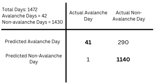
The LSTM classification model for wet slab and glide snow avalanche prediction presented in this paper had a sliding window of 5 days, a weight loss function of 1.0 for non-avalanche days and 5.5 for avalanche days, and a decision threshold of 0.3. As shown in Fig. 1, it correctly predicted 41 of 42 avalanche-days in the training set, missing only 6/13/2020, which was the most commonly missed avalanche day among all hyperparameter configurations. This date corresponds to two glide snow avalanches likely triggered by a warm-up in temperatures, and was most likely misclassified since it occurred in mid-June when avalanches are generally less frequent due to warmer temperatures and lower snow depth.
This specific iteration of the model was chosen to balance avoiding overfitting and minimizing false positives while accurately predicting the vast majority of avalanche days. Table 2 presents the performance on both the training and independent test sets. The training accuracy was 80%, while the test accuracy was 87.16%. The higher test accuracy likely results from temporal differences between the training and test periods, where the test set contained weather patterns more easily classified by the model. It had a test loss of 0.2615, a reasonable value for binary classification problems. These results indicate that the model performs well at correctly classifying “avalanche days” while producing a moderate amount of false positives. When it comes to avalanche forecasting, there are two types of errors to consider with different importance. A false positive will result in heightened awareness for the region on that day, even if no avalanche occurred. A false negative is more severe since an avalanche would occur on a day where no avalanche is predicted, which would pose a significant threat to human safety. Thus, it is desirable to have a higher number of false positives to reduce instances of false negatives.
Given the highly imbalanced nature of the dataset, the overall accuracy metric can be misleading. Instead, several imbalance-appropriate metrics were used to more comprehensively evaluate model performance. The recall was 0.98, meaning that the model correctly predicted nearly all true avalanche days. The balanced accuracy, which averages recall and specificity, was 0.89, indicating strong performance across both classes. Additionally, Youden’s J statistic – a performance metric that balances sensitivity and specificity – was 0.77, which further supports the model’s effectiveness. Precision and F1 scores were lower due to the higher rate of false positives. Overall, the model’s high recall and balanced accuracy suggest that it is well-suited for real-world use, as it predicts most avalanche days while maintaining a reasonable control over false positives.
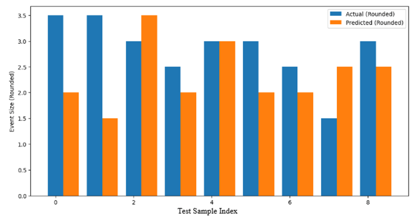
The XGBoost model for predicting the destructive force size of wet slab and glide snow avalanches performed poorly, as indicated by a negative R-squared value and a mean absolute error of 0.83, as visible in Table 3. A negative R-squared implies that the model underperformed compared to a simple mean baseline, indicating it failed to capture meaningful patterns in the data. As shown in Fig. 2, many predictions differed from observed magnitudes by 1.0 – a significant discrepancy given the logarithmic nature of the destructive force scale. This disparity likely resulted from the absence of several influential factors such as avalanche speed, mass, and density, which were not included in the dataset due to practical measurement constraints. Avalanche speed requires in-field observation, and mass depends on snowpack characteristics. Without these variables, predicting destructive force based solely on weather data is inherently limited for wet slab and glide avalanches.
6.2 Wet loose LSTM model analysis and XGBoost model analysis
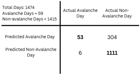
The LSTM classification model for wet loose avalanche prediction presented in this paper had a sliding window of 2 days, a weight loss function of 1.0 for non-avalanche days and 5.5 for avalanche days, and a decision threshold of 0.2. As shown in Fig. 3, it predicted 53 out of 59 avalanche days in the training set, missing six days: 6/10/2020, 4/10/2023, 4/11/2023, 4/16/2023, 4/23/2023, 4/25/2023. These avalanche days were the most commonly missed across all hyperparameter configurations. There was one wet loose avalanche on 6/10/2020 with confirmed date accuracy that had a size destructive force of 1. There was one wet loose avalanche of magnitude 1.5 on 4/10/2023 and three on 4/11/2023 with magnitudes 1.5, 1.5, and 2, all with approximate date accuracies, which suggests that this wet loose avalanche cycle was missed. There were two avalanches on 4/16/2023 with a size destructive force of 1.5. There were six avalanches on 4/23/2023 with two of size 1, three of size 1.5, and one of size 2. There were two avalanches on 4/25/2023 that had destructive forces of 1.5 and 2. All of these missed avalanches had low destructive force sizes, so the patterns in the weather may not have been strong enough to be detected and warrant a prediction. Another interesting observation is that 5 out of the 6 missed avalanche days were within a span of 15 days in the month of April of 2023, and there were no other avalanche days in that month, suggesting that this weather pattern sequence was missed, which could indicate that the model is slightly better at predicting avalanche occurrences based on patterns learned from earlier years. Despite these few omissions, the model captured the vast majority of avalanches with a recall of 0.90, showing that it correctly identified 90% of true avalanche days. It achieved a balanced accuracy of 0.84, which fairly evaluates performance across both classes by averaging recall and specificity (0.79). The Youden’s J statistic was 0.68, showing that the model can distinguish between avalanche and non-avalanche days despite imbalance. As shown in Table 4, the model had a training accuracy of 79% and a test accuracy of 96%. The test accuracy may have been higher than the training accuracy because the testing set contained clearer, more distinguishable weather patterns that were easier to classify. The test loss was 0.359, a reasonable value for binary classification problems. Although precision and F1-score were lower due to a higher false positive rate, this tradeoff is acceptable due to the effects of an avalanche occurring outweighing a false alarm. These results indicate that the model performs well at correctly classifying “avalanche days” while having a balanced number of false positives.
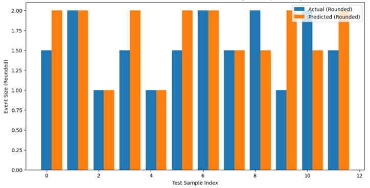
The XGBoost model for wet loose avalanches performs comparatively better on the testing data than the wet slab and glide snow XGBoost, with 5/12 accurate predictions, 6/12 predictions that were off by 0.5, and only 1/12 prediction that was off by 1.0, as can be seen in Fig. 4. A difference of 0.5 in destructive force is acceptable as it still conveys the necessary level of danger and warning. Some instances of these slight differences between predicted and recorded values could have resulted from subjectivity by the recorder, as multiple observation notes indicated uncertainty between two possible values that differed by 0.5. The results in Fig. 4 indicate that to an extent, this model can predict maximum destructive force of a day for wet loose avalanches. Overall, 11/12 of the maximum size destructive force predictions being within a 0.5 range of error is desirable, especially based solely on weather. The feature importance metric for gain, as visible in Table 5, finds that the average air temperature and snow depth are the most significant factors in influencing destructive force size for wet loose avalanches, in that order. The significance of air temperature and snow depth’s influences on wet snow avalanches is corroborated by other papers, including6. However, one unexpected result was that the snow water equivalent was found to be not as important as the other features for wet loose avalanches. This could be because it was measured at the Flattop mountain site, where the snow water equivalent loss may not be consistent with the snow water equivalent loss in the starting zones of avalanches, which tend to be in much higher elevations and may receive more precipitation4.
6.3 Comparisons to other methods
The Random Forest control model, used to predict all types of avalanches, had a testing accuracy of 72.55%, yet it only predicted 10.3% of avalanche days. In contrast, both LSTM models demonstrated significantly higher training and testing accuracies, recall, and balanced accuracies.
For each of the avalanche groupings, separate SVMs were applied as baselines. The wet slab and glide snow avalanche SVM had 994 true negatives, 439 false positives, 2 false negatives, and 38 true positives, resulting in an accuracy of 0.70, recall of 0.95, balanced accuracy of 0.82, precision of 0.08, and an F1-Score of 0.15. The wet slab and glide snow LSTM model had significantly higher scores in all of these metrics. Moreover, McNemar’s test comparing these two models resulted in a test statistic of 331.0 and the p-value of 1.36e-77, indicating a major difference in their predictions.
The wet loose snow avalanche SVM had 1010 true negatives, 437 false positives, 0 false negatives, and 27 true positives, with an accuracy of 0.70, a precision of 0.06, and an F1-Score of 0.11. The wet loose snow LSTM model surpassed these scores and provided better balance between false positives and false negatives. McNemar’s test for these models reported a test statistic of 357.0 and a p-value of 1.996e-72, demonstrating a major difference in their predictions.
Overall, the developed LSTM models effectively predicted the majority of avalanche days and exhibited significant improvements over several baseline models.
Unlike traditional avalanche forecasting methods that heavily rely on expert knowledge and snowpack observations, this study demonstrates that machine learning models, particularly the developed framework, can learn temporal and nonlinear patterns directly from meteorological data. This can be applied to regions where direct snowpack measurements are sparse. While these models are not meant to replace expert forecasters, they can serve as effective complementary tools that can promote safety and advance warning.
Additionally, some avalanche events in the dataset were recorded with approximate dates due to limitations in field observations, particularly for weekend events or remote areas. This temporal uncertainty introduces label noise into the training data, where real-world avalanche days may be misclassified as non-avalanche days and vice versa. This could lead the LSTM classifier to train on misleading examples or result in real-world true positives being classified as statistical false positives, thereby underestimating the model’s actual performance. However, although some estimations may lack precision, these approximations were based on the best judgements of experienced avalanche scientists and so the labeled dates should reasonably be considered representative of actual avalanche occurrences. Nonetheless, future work could benefit from more precise event recording.
6.4 Applications of Proposed Models
The LSTM and XGBoost models for the two groupings as they are could be applied in Glacier National Park and provide advance warning to tourists or maintenance crews traversing the GTSR corridor. These models might also be applicable to other locations along the Rocky Mountains with similar weather patterns if there is access to relevant data. More generally, future studies could develop and train similar models over longer periods of time and in additional geographic regions to further explore the relationship between weather data and avalanche occurrence, while also forecasting avalanche danger and serving communities. Alternatively, researchers may choose to develop localized predictive models for more specific subregions and would incorporate additional features such as slope angles and detailed snowpack measurements.
7. Conclusion
This study examines the effects of weather variables such as air temperature, snow depth, precipitation accumulation, and snow water equivalent on the occurrence and destructive force of wet snow avalanches. Using 21 years of meteorological data, ensemble models were developed to classify avalanche days and predict destructive force for two distinct groupings of wet snow avalanche types: wet slab and glide snow avalanches, and wet loose avalanches. An LSTM model was used for classification, while an XGBoost was applied for regression. These models performed well on the training data and were further validated on the testing data. Compared to previous methods like Random Forest and Support Vector Machines, this approach – utilizing LSTM models and other important tools – led to significantly better predictive abilities.
The XGBoost model for wet loose avalanches achieved predictions close to actual sizes, highlighting the importance of variables like average air temperature and snow depth. This supports the wet loose LSTM model’s predictions by also predicting the extent of danger. However, the wet slab and glide snow XGBoost model showed lower accuracy, likely due to the absence of important factors such as avalanche speed or snowpack density.
By leveraging the LSTM model’s ability to model sequential weather patterns and XGBoost’s strength in regression, this study demonstrates the effectiveness of these machine learning models in avalanche forecasting. Future research could adapt this ensemble approach to different regions and incorporate additional features. Given the devastating impact of avalanches, this approach offers a promising tool for improving forecasting, protecting communities at risk, and mitigating the harmful effects of avalanches.
References
- Stethem, C., Jamieson, B., Schaerer, P., Liverman, D., Germain, D., & Walker, S. (2003). Snow avalanche hazard in Canada – A review. Natural Hazards, 28(2/3), 487–515. https://doi.org/10.1023/a:1022998512227 [↩]
- Reardon, B., & Lundy, C. (2004). Forecasting for natural avalanches during spring opening of the Going-to-the-Sun Road, Glacier National Park, Montana, USA. In K. Elder (Ed.), Proceedings of the 2004 International Snow Science Workshop (pp. 565–581). International Snow Science Workshop Canada. [↩] [↩] [↩]
- Schweizer, J., Jamieson, J.B., & Schneebeli, M. (2003). Snow avalanche formation. Reviews of Geophysics, 41(4). https://doi.org/10.1029/2002rg000123 [↩]
- Peitzsch, E. H., Hendrikx, J., Fagre, D. B., & Reardon, B. A. (2012). Examining spring wet slab and glide avalanche occurrence along the Going-to-the-Sun Road corridor, Glacier National Park, Montana, USA. Cold Regions Science and Technology, 78, 73–81. https://doi.org/10.1016/j.coldregions.2012.01.012 [↩] [↩] [↩]
- Reardon, B., & Lundy, C. (2004). Forecasting for natural avalanches during spring opening of the Going-to-the-Sun Road, Glacier National Park, Montana, USA. In K. Elder (Ed.), Proceedings of the 2004 International Snow Science Workshop (pp. 565–581). International Snow Science Workshop Canada. [↩]
- Součková, M., Juras, R., Dytrt, K., Moravec, V., Blöcher, J. R., & Hanel, M. (2022). What weather variables are important for wet and slab avalanches under a changing climate in a low-altitude mountain range in Czechia? National Hazards and Earth System Sciences, 22, 3501–3525. https://doi.org/10.5194/nhess-22-3501-2022 [↩] [↩]
- Breiman, L. (2001). Random Forests. Machine Learning, 45(1), 5–32. https://doi.org/10.1023/a:1010933404324 [↩]
- Williams, K. (1998). An overview of avalanche forecasting in North America. In Proceedings of the 1998 International Snow Science Workshop, Sunriver, Oregon (pp. 161–169). International Snow Science Workshop. https://arc.lib.montana.edu/snow-science/objects/issw-1998-161-169.pdf [↩]
- Choubin, B., Borji, M., Mosavi, A., Sajedi-Hosseini, F., Singh, V. P., & Shamshirband, S. (2019). Snow avalanche hazard prediction using machine learning methods. Journal of Hydrology, 577, 123929. https://doi.org/10.1016/j.jhydrol.2019.123929 [↩]
- Mayer, S., Techel, F., Schweizer, J., & van Herwijnen, A. (2023). Prediction of natural dry-snow avalanche activity using physics-based snowpack simulations. Natural Hazards and Earth System Sciences, 23(12), 3445–3465. https://doi.org/10.5194/nhess-23-3445-2023 [↩]
- National Resources Conservation Service. (n.d.). Air & water database public reports. U.S. Department of Agriculture, National Water and Climate Center. https://wcc.sc.egov.usda.gov/nwcc/site?sitenum=482&state=mt [↩]
- Peitzsch, E.H., Miller, Z.S, & Milone, K.M. (2020). Avalanche occurrence records along the Going-to-the-Sun Road, Glacier National Park, Montana from 2003-2024 (ver. 4.0, November 2024). U.S. Geological Survey. https://doi.org/10.5066/P9BO1LHQ. [↩]
- Rengasamy, D., Jafari, M., Rothwell, B., Chen, X., & Figueredo, G. P. (2020). Deep learning with dynamically weighted loss function for sensor-based prognostics and health management. Sensors, 20(3), 723. https://doi.org/10.3390/s20030723 [↩]
- Esposito, C., Landrum, G. A., Schneider, N., Stiefl, N., & Riniker, S. (2021). GHOST: Adjusting the decision threshold to handle imbalanced data in machine learning. Journal of Chemical Information and Modeling, 61(6), 2623–2640. https://doi.org/10.1021/acs.jcim.1c00160 [↩]


