Design and Preliminary Testing of a Drone-Mounted Water Delivery Prototype for Individual Plants

Abstract

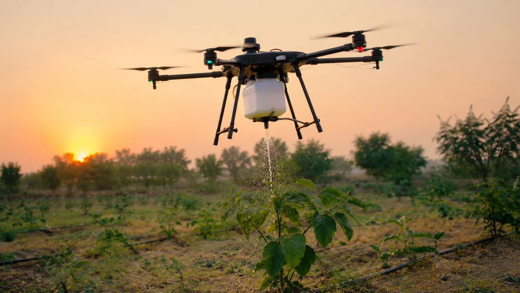
Hand-watering in a UAE school garden is slow, and the water every plant gets is estimated by eye. This study investigates whether a small quadcopter can be equipped with a removable water-delivery payload and its pump switched by a soil-moisture reading taken at the target plant. A small 3D-printed reservoir, a 12 V pump, silicone tubing and a brass nozzle were attached under the bottom of a DJI Mavic 2 Pro. A ground ESP32 read a capacitive soil probe and sent a normalized moisture index every second over ESP-NOW to an airborne ESP32. The airborne ESP32 switched the pump via a MOSFET: below 30% moisture the pump was switched on, and it was switched off at 45% or after 3 s without any data. In total 8 bench pump trials, 5 dry and 5 wet reference readings, 6 ground watering runs wit258h 4 controls, 9 manual flights with 250–750 mL water in the payload and 6 integrated flights with the sensor link active were performed. Bench flow averaged 8.58 mL/s (SD 0.15 mL/s). In all 12 runs (6 ground + 6 integrated flights) the pump started only below 30% moisture and was switched off at 45.4–48.2% moisture. All 4 controls for the ground watering runs stayed off. All 15 flights were completed without loss of control. However, the calculated take-off masses of 1,557–2,057 g were 1.7–2.3 times the take-off mass of 907 g specified by the manufacturer. The pilot described reduced vertical response at higher loads. Thus, while this study’s prototype demonstrates sensor-switched aerial water release as opposed to precision irrigation, several key aspects, i.e. target capture, water savings and a safe payload, remain to be measured.

Keywords: Unmanned aerial vehicle; irrigation; capacitive soil moisture sensor; ESP32; ESP-NOW; payload mass; school garden.

Introduction

Background

Freshwater is unevenly distributed around the world. A large portion of the world’s population faces severe water scarcity for at least one month of the year, estimated to be around four billion people by Mekonnen and Hoekstra¹. With the projected growth of the world population to reach 9.7 billion in 2050 and to peak at 10.4 billion in the 2080s², the challenge of growing enough food using limited water is real and needs to be addressed. The most practical solution to using irrigation water is to apply it where and when plants need it, i.e. at large farms or even in small gardens.

In the first place this is a local problem in the sense that the Eco-Committee of our school is taking care of the school garden. This garden has to be watered all year round, especially in the hottest and driest months of the year in the UAE. Up to now this has to be done by hand and depends on students and staff members who voluntarily spend their time to water the plants. They try to give the right amount of water to the individual plants but they have to rely on their eyes as no measuring is done.

Related Work

Automatically controlling irrigation based on measurements of soil moisture is a common practice for systems on the ground. In a field study of bermudagrass plots, three commercial systems for controlling irrigation based on soil moisture reduced irrigation by 69% to 92% without reducing turf quality³; in a study of 58 homes, sensor-controlled irrigation reduced water application by 65% compared with the homes using only a timer to control irrigation⁴. A field comparison of four commercially available systems found that on average the sensor-based treatments skipped about 71% of the irrigations that would have been made using a fixed time schedule, however most of the sensors did not provide consistent accurate readings, and the decisions made by the sensors for a given soil moisture reading sometimes differed⁵. Schemes that cost less than the commercially available systems can be implemented using an Arduino or ESP32 based microcontroller, an inexpensive soil moisture sensing probe, and a 12V relay to switch a pump⁶; larger Internet-of-Things (IoT) based systems that include remote monitoring and control of the irrigation also are available⁷.

The primary problem for most sensor-based watering controllers is the sensor itself. A capacitive probe in the soil measures the soil surrounding the probe, thus the readings are dependent on the soil’s texture, compaction, and salinity, as well as its water content^8,9. Further, there is an effect of temperature on the probe’s readings¹⁰. This type of sensor also is not very consistent between like sensors⁸. For example, variations of greater than 5% have been reported between two nominally identical probes of the same model⁸. Similar results have been found with other low-cost, capacitive-type sensors^9,11. After soil-specific calibration, however, low-cost capacitive sensors have matched a secondary-standard sensor in the laboratory¹² and a commercial sensor in the field¹³, and calibration equations have been published for the widely used SEN0193 probe in organic and loamy-silt soils^14,15.

Spraying crops using UAVs is currently practiced but not for irrigation. For example, a system was tested for control of aphids on wheat and found to perform as well as boom or knapsack sprayers and was up to 20 times faster than them. However, the deposition was not very uniform with a coefficient of variation of 87.2% for the UAV system and 31.2% for the boom sprayer¹⁶. Other factors that affect the deposition of UAVs sprayers include flight height^17,18, droplet size¹⁹, and canopy characteristics¹⁸. In some applications, small UAVs are retrofitted with sprayers for ultra-low-volume applications on small targets in orchards such as olive and citrus trees²⁰. The amount of carrier water used for spraying using UAVs is far less than that used for ground-based systems. For example, in a study on maize, a UAV was used for foliar application of a nano-urea fertilizer spray using 25 L ha−1 of water as carrier as opposed to 500 L ha−1 of water used as carrier in a tractor-mounted gun sprayer. The yields were not significantly different (mean ± SE, 2,928 ± 503 and 2,912 ± 375 kg ha−1; p = 0.98) for the two methods of spraying in the study with five replicates, although a non-significant result from five replicates does not by itself show that the two methods are equivalent²¹. In a life-cycle assessment study of wheat spraying, it was found that conventional spraying used 2.43 times more energy per hectare than drone spraying of wheat²². Reviews have described the current state of the art in the navigation and vision systems used for spraying UAVs²³. These studies, however, relate to the amount of water used as a carrier for fertilizers and pesticides and not to the amount of water that a crop requires for irrigation.

UAVs have been associated with irrigation mostly in the frame of sensing and monitoring. UAV-borne thermal sensors were used to map water status of individual trees within two 130-ha fields of a pistachio farm and manage irrigation on management unit level²⁴. A pilot study was conducted in Saudi Arabia in which a UAV was outfitted with sensors to measure temperature, humidity and soil moisture across the farm. Data collected were processed in cloud-based service to determine the amount of water required for irrigation in different sections of the farm and the information was sent to ground-based pumps supplying water to the relevant sections of the farm²⁵.

Problem Statement and Rationale

Most studies on UAVs for agriculture used either UAVs to spray a whole field with agrochemicals or used a UAV for sensing the crop water status and then used ground-based controllers to decide on and control the required amount of water for irrigation. We couldn’t find any study that used a small quadcopter to carry and deliver water to individual plants based on soil sensors located at the roots of the plants. Such a system would have the advantage of the threshold values used by ground-based controllers and the mobility of an aircraft. However, there are three questions that have not been answered by the spraying and sensing studies. First, there is the issue of mass: the power required to fly a multirotor increases roughly linearly with mass of the airframe, rotors, and batteries, plus the mass of any payload carried²⁶, and flight tests of a delivery quadcopter showed that heavier payloads increase the energy used per trip²⁷. Different studies have found very different energy use for a variety of aircraft under a variety of conditions²⁸. The second issue is communication: the sensor is located in the soil and the pump is located on the aerial vehicle, thus some form of wireless communication is required. ESP-NOW, a connectionless communication method for the ESP32 board, was found to communicate over long distances of up to 185 m in comparison with Wi-Fi at 84 m and Bluetooth at only 15 m in a test of communication over distance using identical hardware and software²⁹. However, a test of the same communication method in an actual field found that the % packet delivery was >99% up to 56 m but then began to drop sharply³⁰. The third, and probably most difficult to solve, issue is delivery efficiency: how much of the water that is released from the nozzle of the hovering quadcopter actually ends up in the root zone of the individual plant?

Objectives and Scope

This study aimed to design a water-delivery payload, easily removable from a quadcopter and connected to a soil sensor that controls the pump. The objectives of this study were to 1) build and weigh all the airborne parts of the water-delivery payload, 2) measure the flow rate of the pump on the bench, 3) characterize the soil probe using dry and wet references, test a start–stop threshold on the ground, 4) test the payload with increasing amounts of water and 5) test the full chain of soil reading, wireless transmission and aerial pumping in flight. The study used one aircraft, one pump, one soil probe and one school garden. It did not measure the fraction of the water that was released that actually reached the plant, compared the water use to that of manual watering or established a safe maximum mass for the payload. Thus the study only establishes the feasibility of such irrigation systems and does not measure their accuracy or water saving potential.

Theoretical Framework and Approach

In on–off control with hysteresis the irrigation is switched on when the moisture index falls below a lower threshold and is switched off when the moisture index reaches the upper threshold. Thus small deviations from a set point do not result in the pump being switched on and off. This is in contrast to the single-threshold-logic of commercial soil-moisture-sensor controllers, which skip a scheduled irrigation if the soil moisture is above a predefined threshold⁵. The amount of water that is delivered by the irrigation is calculated as flow rate times pump-on time (Equation 4). This model is discussed in more detail below. As mentioned before, the development of the controller was done in stages, i.e. one subsystem after the other.

Methods

Research Design

The study reported here is an experimental engineering study conducted in stages. Initially the individual parts or subsystems of the system under investigation were tested on the workbench (B-series): the pump, dry and wet reference readings of the soil probe. Subsequently ground tests of the control rule were conducted (S-series) followed by loaded flights of the aircraft (F-series). The final stage of the study comprised integrated flights with the sensor link switched on (I-series). There were no human or animal subjects in this study. The target organisms were six potted Ocimum basilicum (basil) plants grown in commercial potting mix in the school’s Eco-Committee garden.

Aerial Platform

The aircraft used for the tests was a DJI Mavic 2 Pro, a small, folding, camera-equipped quadcopter with a take-off mass of 907 g and a hovering time of 29 min without any payload³¹. The drone was chosen because it was already available to the author for zero cost, is small enough to fly between individual garden beds and thus allows the main load (i.e. the payload) to be tested rather than the entire airframe. Importantly, however, DJI does not rate the Mavic 2 Pro for payload, so any water carried adds to a mass the aircraft was not designed to lift. Thus, the flights were conducted using partial loads of water, ranging from 250 mL to 750 mL, rather than the full design capacity of the test reservoirs. The aircraft was flown manually, within the pilot’s visual line of sight; no autonomous, GPS-guided, waypoint-based flights were made.

Payload Design

The assembled payload is shown in Figure 1. The airborne articles are listed in Table 1 with their models, ratings, and masses. The reservoir was designed in CAD and 3D printed in PLA as separate parts which could be printed by the printer. The design capacity of the reservoir is about 1 L or 1 kg of water, but the amount of water to be placed in the reservoir for the tests was limited to the amount required for the test. The water load is positioned as low as possible with respect to the centre of gravity by placing the reservoir below the body of the aircraft. The reservoir is held in place by custom clamps which are attached around the four landing legs of the aircraft. The payload can be removed from the aircraft without damaging the airframe.

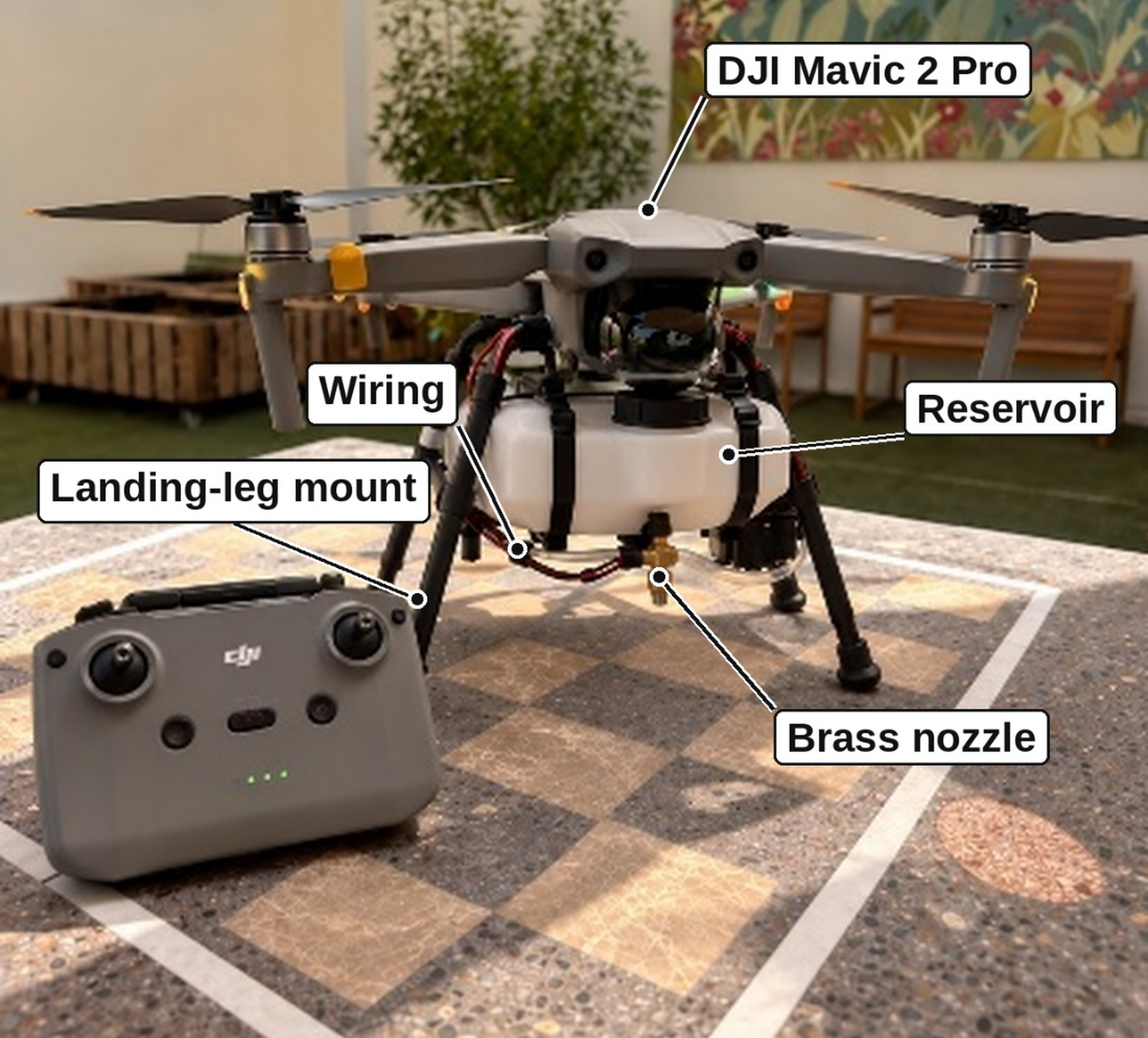
In the built system, water is moved by a single 12 V DC pump via some silicone tubing to a single brass nozzle where it is concentrated onto the target plant part. Water leaves the nozzle only while the pump is running. There is one soil probe, one pump, one nozzle, and no valves.

Component	Qty	Model/ part number	Key rating	Mass (g)
DJI Mavic 2 with flight battery	1	Mavic 2 Pro	No payload rating published	907.0
3D-printed leg clamps and mounts	1	Custom; PLA	—	74.6
Reservoir with fittings (empty)	1	Custom; PLA	≈1 L design capacity	61.8
12 V DC pump	1	R385 diaphragm water pump	1.5–2.0 L min⁻¹; 0.5–0.8 A	63.7
Silicone tubing	1	6 mm ID; 0.50 m length	—	8.4
Brass nozzle with fittings	1	Brass misting nozzle	0.5 mm orifice diameter	22.7
Airborne ESP32 board	1	ESP32-WROOM-32 DevKit V1	3.3 V logic outputs	10.1
MOSFET module	1	IRLZ44N MOSFET module	VGS(th) 2–4 V; max. current 9.2 A	7.6
Buck converters (A ≈12 V; B ≈5 V)	2	LM2596 DC-DC step-down module	3 A max. output current	15.8
Auxiliary Li-ion battery	1	4S Li-ion battery pack	14.8 V nominal; 2200 mAh	106.4
Wiring, connectors and fasteners	—	22 AWG stranded copper wire	—	28.9
Dry payload (all items except the aircraft)				400.0
Aircraft and dry payload				1,307.0

Control Electronics

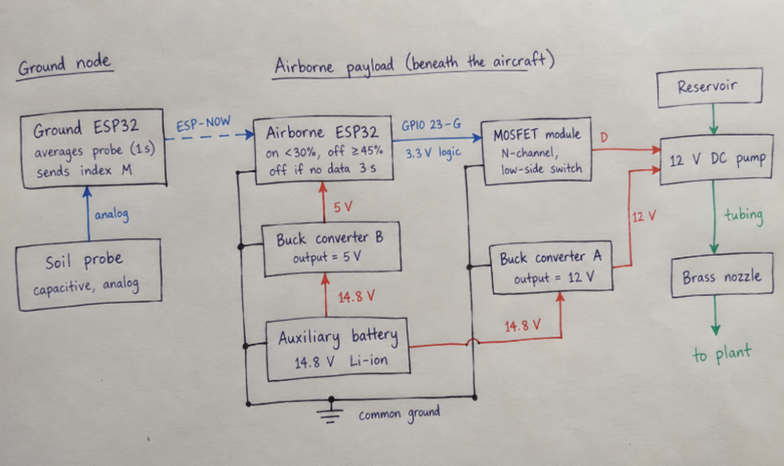
The board at the ground has the soil probe for the reading of the soil moisture, it sends the acquired values to the airborne ESP32 using the method ESP-NOW. The board at the ground has also its own regulated low-voltage power supply. The airborne board receives the readings and it is used for switching the pump. On the aircraft there is used a separate 14.8 V nominal lithium-ion battery (Figure 2), that is different from the flight battery of the aircraft. This battery is used for two buck converters. Converter A is used for the production of a voltage of about 12 V, which is then used for the pump, while Converter B produces a voltage of about 5 V, which is then used for powering the airborne board.

The IRLZ44N N-channel MOSFET module was used to switch the pump on the low side. The MOSFET connects the negative side of the pump to ground, while the positive side of the pump stays connected to the 12V supply. The Gate of the MOSFET is connected to GPIO 23 on the airborne ESP32 module. The ESP32 module operates from a 3.3V logic supply, and hence requires the MOSFET to switch fully on at a gate–source voltage of 3.3V. The IRLZ44N is a logic-level device. The gate threshold voltage is specified to be in the range 1.0–2.0V, and the maximum on-resistance is specified to be 0.035Ω at the lowest gate voltage listed in the data sheet. Given that the pump draws approximately 0.8A, this is quite sufficient. A 1N5819 Schottky flyback diode was placed across the motor terminals to prevent voltage spikes from damaging the IRLZ44N FET when the motor switched off. The ground connection for the battery negative terminal, the two power converters, the ESP32 module, and the source connection of the IRLZ44N FET all share a common point, the ground for the 3.3V gate signal is therefore referenced to the same point as the pump current.

Soil-Moisture Sensing and Control Logic

This ground node uses a capacitive soil probe (Capacitive Soil Moisture Sensor v1.2) inserted into the soil 5 cm down from the surface and about 5 cm from the stem of the plant it is monitoring. It samples the analog output of the probe every 100ms. The readings are averaged over 10 readings taken over 1.0s and then converted to a normalized moisture index:

M was expressed as a percentage of the span between the two reference conditions (0% for the dry reference and 100% for the wet reference). Note that M is a relative index for this probe in this potting mix and not a volumetric water content. It was not possible to use the probe to measure the volumetric water content of the soil because it was not calibrated using gravimetric or volumetric samples of soil. The means of the dry and wet reference readings for ADC (ADCdry and ADCwet) were 3191 and 1428 respectively (Results).

The ground node periodically sends ESP-NOW packets containing sequence numbers, the mean ADC value, M, and the status of the pump request. The airborne node then applies the control rules: after two consecutive values below 30% the pump starts to pump, and it stops pumping after the first valid reading of 45% or higher (hysteresis band of 15 points). If no valid ESP-NOW packet is received for more than 3.0 s, the GPIO 23 of the airborne node is set to low, so that the pump is switched off until valid readings are received again. The values of 30% and 45% are values on the relative index of Equation 1 and not water contents.

Construction and Assembly

The CAD model was split into two printable parts for the reservoir and the clamp. The tubing and the nozzle were assembled together. The ESP32–MOSFET switching circuit for the water pump was wired up. The two buck converters were tuned to the correct output voltages for the pump. The completed assembly was then attached beneath the airframe. As each section was completed problems with the design were exposed, such as leaks at connections for the tubing, lack of space for mounting points, routing wire safely round the rotors, additional weight reducing flight time, and the vibration causing problems to the pump. These were all solved prior to commencing work on the next section.

Mass Budget

All airborne parts, the two converters and the wiring with all connectors and fasteners were weighed in groups on a digital balance with 0.1 g resolution. The dry payload has a mass of 400.0 g. The mass of the whole aircraft including the flight battery and dry payload was 1,307.0 g. The ground based ESP32 and the soil probe stay on the ground. Taking the density of water to be 1.00 g mL−1, the take-off masses for 250 mL, 500 mL and 750 mL of water are 1,557 g, 1,807 g and 2,057 g, respectively. In relation to the take-off mass of 907 g specified by the manufacturer of the aircraft this translates into 1.72, 1.99 and 2.27 times the specified mass. However, the manufacturer does not specify a payload for the aircraft and thus the figures above do not represent a safe payload.

Test Procedures

Table 2 summarizes the five test series, the number of runs in each and the quantities recorded.

Series	Runs	Conditions	Recorded	Not measured
B: bench pump	8	Pump on bench; 500 mL start	Pump-on time; collected volume	—
Sensor reference	5 dry + 5 wet	Probe in dry and in wet soil	ADC count	Volumetric water content
S: ground control	6 + 4 control	Control rule on the ground	ADC and M at start and shut off; pump-on time; water delivered	Water reaching root zone
F: load flights	9	Manual flights; 250, 500, 750 mL	Pump-on time; discharged volume; duration; displayed battery %; pilot notes	Water reaching plant
I: integrated flights	6	Manual flights; sensor link active	ADC and M at start and shut off; pump-on time; duration; displayed battery %	Delivered volume(estimated); water reaching plant; packet loss

Bench pump tests (B-series)

We measured the unmounted pump’s discharge before attaching it to the test rig. We repeated this measurement eight times. For each measurement we filled the reservoir to 500 ± 5 mL and then ran the pump for a set time of 10–40 s (measured by hand with an error of ±0.2 s). The discharged water was collected in a graduated vessel with an error of ±5 mL.

Sensor reference readings

For the dry reference readings, samples of the same commercial potting mix used for the basil plants were air-dried over 48 hours prior to measurement. For the wet reference readings, the same potting mix was slowly saturated with water until the mix was evenly wet but with no sign of surface water. The probe was withdrawn from the soil, cleaned and then reinserted to the same depth of 5 cm between individual readings. The mean of the dry readings and the mean of the wet readings formed the end points of the index (Equation 1).

Ground control tests (S-series)

To test the control rule on the ground, the assembled payload was placed on a test stand next to a potted target plant. The probe was inserted into the soil about 5 cm deep and about 5 cm away from the plant stem. Six runs tested the control rule starting with a soil index well below 30%. The readings from the ground node then switched the pump on and off automatically. The ADC counts and corresponding indexes at the start and end of the pump period, the duration that the pump was on and the amount of water delivered by the pump were all recorded. The water delivered by the pump was calculated as the difference between the reservoir volume before the run and the volume remaining after the run. This volume was measured using the same graduated vessel (±5 mL) as for the bench tests. For four additional control runs the soil index started well above the 30% start threshold and the expected action was for the pump to remain off.

Loaded flights (F-series)

A total of nine flights with manually piloted loaded UAS were conducted to test the loaded aircraft, with three flights of each 250 mL (F1–F3), 500 mL (F4–F6) and 750 mL (F7–F9) of water. Flight F1 was a hover only test without any water pumping. For the remaining flights, F2–F9, a manual switch of the pump by the ground node was commanded by a timed command, independent of the control link to the soil sensors. The flights were all conducted within the covered courtyard of the test garden and all flights hovered approximately 1.0 m above the target plant. The time taken to fly from take-off to landing for each flight, plus the before and after battery percentage for each flight, were recorded from the DJI app by the pilot. The volume of water discharged was calculated as the initial volume of water in the reservoir minus the residual volume of water after the flight, both measured using the graduated vessel to the nearest 5 mL. The pilot also noted any changes in handling the aircraft.

Integrated flights (I-series)

All parts of the control chain were tested with six flights, two of them at each of the three water loads. The flights started with the aircraft hovering above a test plant whose initial index was below 30%, about 1.0 m from the ground node. During the flights the ground ESP32 was sending the sensed values to the airborne ESP32 by ESP-NOW. The airborne ESP32 then controlled the pump according to the above defined control rule. The following values were recorded during the flights: ADC count and Index at start of pump run and at shut-down of the pump, duration of pump run, flight duration, battery usage in percent. The remaining volume in the reservoir after the flight was not recorded, thus the delivered water was calculated from the duration of the pump run (Equation 4).

Success criterion

A flight was scored as successful, if it took off and landed properly, hovered above the target, completed the planned activity (pumping water or hovering in the case of the F1 design) and was under the pilot’s control the whole time. This measure of success was applied to the flight log after the test had taken place. It merely describes flight feasibility, and was not intended to determine the proportion of water delivered to the plant or the degree of targeting accuracy.

Data Analysis

For each bench trial, the mean flow rate was calculated from the collected volume and the pump-on time:

where Q is the mean flow rate (mL s−1), V the collected volume (mL) and t the pump-on time (s). Equation 2 is the definition of average flow rate, not a characteristic curve of the pump. The reading uncertainty of each trial was propagated as

with u_v = 5 mL and u_t = 0.2 s. Water delivered in the I-series was estimated as

Bench mean flow was rounded to one decimal place and hence equals 8.6 mL s−1 for all calculations of Qmean in Equation 4. The filling of the tubing and motor spin-up, as well as the falling pressure head in the reservoir as it empties, together with a decrease in battery voltage and finally dripping after shut-down could all have resulted in a different volume being delivered than that calculated using Equation 4, particularly for short pulses. The change in index for each series of measurements was calculated as ΔM = Mstop − Mstart. The means, SD and ranges for each series of measurements are provided. Correlation between two variables was expressed using the Pearson correlation coefficient r.

Safety, Authorization and Ethical Considerations

All flights were conducted in the school’s Eco-Committee garden in the covered courtyard of the school. Permission to use the grounds was granted by the school administration and faculty supervisor of the Eco-Committee Project. In Dubai, the operations of unmanned aircraft are governed by the Dubai Civil Aviation Authority (DCAA) under the laws of Dubai (Law No. 4 of 2020)³² within the national framework of Federal Decree by Law No. 26 of 2022 on the civil use of drones³³. However, separate permission from the school was required for the use of school grounds, which was granted by the school administration. Accordingly, all flights were conducted under DCAA Permit No. DCAA-UAS-2026-0417. Due to the addition of payload(s) to the aircraft, the modified aircraft was flown at reduced height (maximum of 2.0 m above ground level) and within Visual Line of Sight (VLoS) of the pilot(s). Prior to each flight, the area was checked for any people, animals or obstacles and appropriately cleared. A maximum of three team members attended each flight and maintained a safe distance of at least 5 m from the aircraft at all times. No people or animals participated in the research as subjects.

Results

Bench Pump Tests

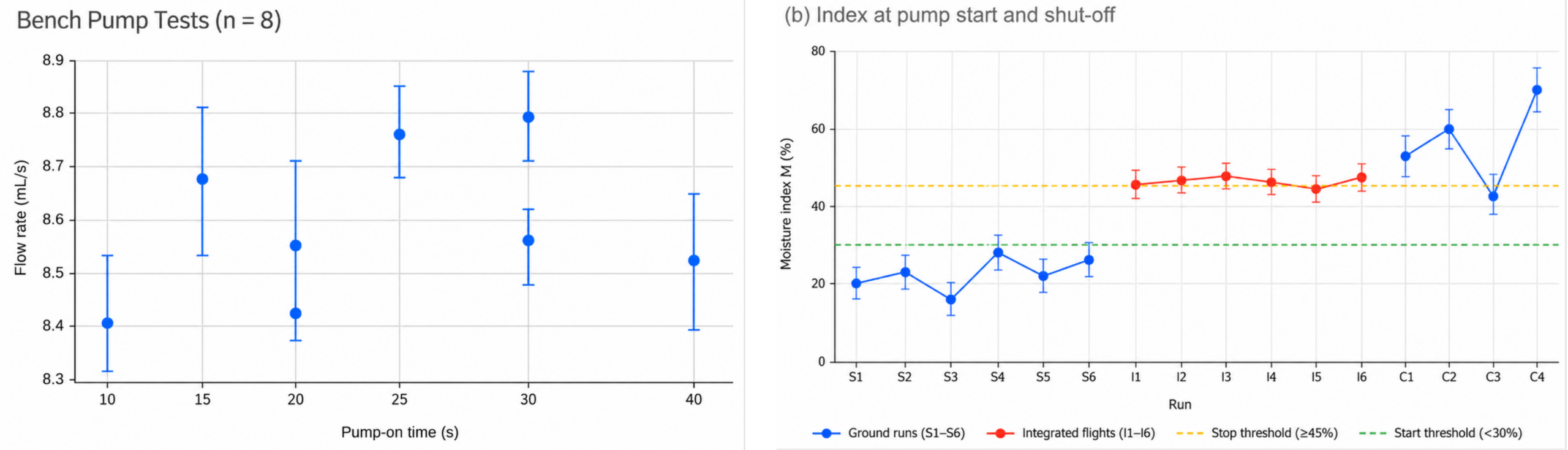
The eight bench trials collected 84–341 mL in 10–40 s (Table 3). Flow rates ranged from 8.40 to 8.80 mL s⁻¹, with a mean of 8.58 mL s⁻¹ and a sample SD of 0.15 mL s⁻¹ (coefficient of variation 1.7%; Figure 3a). The reading uncertainty of individual trials was ±0.13 to ±0.53 mL s⁻¹, largest for the shortest trial, so the spread between trials was within the uncertainty of the measurements. Flow rate did not change systematically with pump-on time (r = 0.31, n = 8).

Trial	Pump-on time(s)	Collected(mL)	Flow rate (mL s-1)	Uncertainty(±mL s-1)
B1	10	84	8.4	0.53
B2	15	130	8.67	0.35
B3	20	171	8.55	0.26
B4	25	219	8.76	0.21
B5	30	257	8.57	0.18
B6	20	168	8.4	0.26
B7	30	264	8.8	0.18
B8	40	341	8.53	0.13
Mean (SD)			8.58(0.15)

Sensor Reference Readings

The five dry readings averaged 3191 counts (SD 25) and the five wet readings 1428 counts (SD 17; Table 4). Wetter potting mix gave lower counts, as reported for other low-cost capacitive probes¹¹. The span between the two means was 1763 counts, so the scatter of repeated readings corresponded to 1.4% (dry) and 0.9% (wet) of the index scale, far smaller than the 15-point gap between the start (30%) and stop (45%) thresholds.

Reading	Dry potting mix (ADC)	Wet potting mix (ADC)
1	3196	1428
2	3158	1451
3	3221	1407
4	3174	1436
5	3207	1419
Mean	3191	1428
SD	25	17

Ground Control Tests

For the six ground runs the pump started at an index of less than 30% (starting index 15.8–28.1%) and automatically switched off at an index of 45.4–48.2% (increase of 0.4–3.2 index points above the stop threshold, Table 5; Figure 3b). The pump was switched on for 12.7–21.8 s and a total of 109–187 mL of water was released. In comparison, drier soil required longer periods of pumping with the duration of pumping decreasing with an increase in the starting index (r = −0.997, n = 6). The amount of water released per point of index increase was 5.7–6.3 mL. All four control runs were started at high indices of 41.4–71.3% and the pump did not switch on at all.

Run	Start ADC	Start M (%)	Pump-on (s)	Water (mL)	Stop ADC	Stop M (%)	Pump response
S1	2847	19.5	18.6	159	2356	47.4	Automatic stop
S2	2774	23.7	15.9	136	2381	45.9	Automatic stop
S3	2913	15.8	21.8	187	2342	48.2	Automatic stop
S4	2696	28.1	12.7	109	2375	46.3	Automatic stop
S5	2818	21.2	17.4	149	2362	47.0	Automatic stop
S6	2741	25.5	14.8	126	2390	45.4	Automatic stop
C1	2257	53.0	0	0	—	—	Stayed off
C2	2118	60.9	0	0	—	—	Stayed off
C3	2461	41.4	0	0	—	—	Stayed off
C4	1934	71.3	0	0	—	—	Stayed off

Loaded Flights

All flights of the F-series were successful (9/9; see Table 6). The duration of the flights varied from 2 min 18 s (F1) to 3 min 54 s (F9). The change in the displayed battery charge of the aircraft for the F-flights varied from 10 % to 31 % and increased with increasing water load of the payload. The mean decrease of the battery charge per minute of the flights with water load increased from 4.7 %/min over 6.3 %/min up to 7.7 %/min for the flights with 250 ml, 500 ml and 750 ml water load respectively. The take-off mass of the aircraft for the three flights with water load was 1.72, 1.99 and 2.27 times the specified mass of the unmodified aircraft, respectively. Note that no flights without any payload were executed to determine the additional battery consumption caused by the payload. As mentioned before the pilot experienced longer times for vertical response for F4 and increased control activity for F7. The volume of water that was pumped and that flowed through the pipes of the pump for all flights of the F-series was measured. For the pump running for 15 s to 45 s the discharged water volume was measured to range from 129 ml to 381 ml respectively. Note that all this water, however, was not collected at the plant under test.

Flight	Water-load (mL)	Pump-on (s)	Discharged (mL)	Duration (min/s)	Battery start→ end(%)	Pilot’s note
F1	250	0	0	2:18	97→87	Hover only; stable
F2	250	15	129	2:46	95→82	Airborne discharge
F3	250	25	214	3:07	96→80	No visible leakage
F4	500	20	169	2:51	94→77	Slower vertical response
F5	500	32	274	3:28	96→74	Watering run completed
F6	500	41	348	3:54	95→69	No pump interruption
F7	750	20	168	2:37	97→78	Greater control correction
F8	750	36	306	3:21	96→70	Irrigation pass completed
F9	750	45	381	3:48	95→64	No loss of control

Integrated Flights

All six I-series flights were fully successful (6 of 6; Table 7). In each of the flights the index value when pumping started was below 30% (16.7–27.3%) and the index value when stopping was 45.4–47.8% (0.4–2.8 points above the stop threshold). In no case did the 3.0 s communication timeout expire, so no instances of pump interruption due to loss of the ESP-NOW link occurred. The pump-on time was 12.4–21.7 s and hence, in accordance with the measurements on the ground, the estimated water volume (using Equation 4) was 107–187 mL. The duration of the flights was 167–232 s, and the measured decrease in charge of the battery was 13–30%. As the estimated volume was derived from the pump-on time only, this volume cannot be used to check the flow rate. Also, the fraction of the pumped volume that actually reached the plant was not measured.

Flight	Load (mL)	Start ADC	Start M (%)	Pump-on (s)	Est. water (mL)	Stop ADC	Stop M (%)	Duration (min/s)	Battery
I1	250	2770	23.9	15.1	130	2390	45.4	2:47	96→83
I2	250	2709	27.3	12.4	107	2384	45.8	3:02	95→80
I3	500	2828	20.6	17.8	153	2366	46.8	3:14	96→77
I4	500	2875	17.9	20.5	176	2358	47.2	3:39	94→71
I5	750	2750	25.0	14.4	124	2388	45.5	3:18	97→75
I6	750	2897	16.7	21.7	187	2348	47.8	3:52	95→65

Discussion

Pump Flow and the Dose Model

Bench trials confirmed that, under the conditions of the bench trials, the pump delivered a constant flow rate. The spread of the flow rate for the bench trials (SD 0.15 mL s−1) was similar to the uncertainty in the measurement of flow rate, and there was no change in the flow rate with pulse length in the range 10 s to 40 s. A constant-flow dose model (Equation 4) is therefore a reasonable first estimate under the conditions of the bench trials. The flow rate measured in the bench trials was in the order of 0.52 L min−1, i.e. well below the rated flow of the pump of 1.5–2.0 L min−1 (Table 1) due to restriction by the tubing and the nozzle outlet. The main variations to consider for flight tests are the initial volume of water in the I-series, the pressure head at the pump, the supply voltage of the pump, the delay in filling the tubing, the spin-up of the motor and any ‘drip’ of water after shut-down of the pump. None of these effects was isolated here. To calculate the dose delivered in flight tests, i.e. the amount of water added to the root zone, it is necessary to measure the amount of water released by the pump and to place containers to collect this water around the target plant(s). These containers can also be used to calculate the fraction of added water that actually penetrated the root zone.

Sensor Index and Thresholds

The two reference conditions were far apart (1763 counts) whereas the standard deviation of the replicated measurements (e.g. 17 counts for wet potting mix) created a cloud of reading values around the mean for the same condition. Hence the probe clearly distinguished between dry and wet potting mix and the two thresholds of 30% and 45% were well apart relative to the spread of reading values. Note, however, that such an index is only a relative scale. Low-cost capacitive soil probes respond to soil texture, compaction, salinity and temperature and each such probe is somewhat different from unit to unit^8,9,10. Therefore such probes only provide correct water content after soil-specific calibration^12,13,14. Thus the two thresholds given here are for that particular probe in that particular potting mix only and cannot be converted into water content or used for any other soil without first having been calibrated for that other soil.

Control Behaviour

In ground tests the hysteresis rule functioned as expected, that is the pump was not started above a moisture level of 30% and the pump was switched off at or just above a moisture level of 45%. As expected, the pump stayed off in all 4 control runs. One control run (C3, index 41.4%) started with the plant in the hysteresis band between the two thresholds. The pump-off margin of 0.4–3.2% is a function of the one-second update interval of the sensor. This means that as long as the water is flowing, it will take one additional packet read before the index value has increased to the threshold value of 45%. In the ground tests the pump-on time decreased in a nearly linear fashion as the initial index increased, while the amount of water added in relation to the increase in soil moisture content of the test cases (5.7–6.3mL/%) was similar. Hence, in principle, a controller could dose water in relation to the remaining moisture deficit instead of using a fixed upper threshold. In field tests, similar ground-based soil-moisture controllers have been shown to substantially reduce irrigation without causing any damage to turf in long-term comparisons with traditional timer-driven schedules^3,4. However, the water savings found in these studies were determined over months, whereas the present study included only very short tests per plant and no comparison with manual watering, so no water saving can be claimed. A field test of commercial soil-moisture controllers found that some sensors made different decisions at the same reading⁵. Repeated measurement of the same probe would help to determine if this probe is consistent or not.

Wireless Link 

By placing the decision at the ground node and having the sensor reading be transmitted to the aircraft, the question of how soil sensor data could possibly get to a controller in the air is answered. Using ESP-NOW allowed for communication of the packets to take place without the need for a router. The data was able to be transmitted at a single packet per second over the short distances used and fell well within the reported ranges for the single ESP32 boards^29,30 used. However the outdoor study did see that packet delivery fell off sharply from above 99% to zero over a few tens of meters towards the edge of the useful range³⁰. A timeout of 3.0 s was placed on the link to stop the pump in case of a lost link but the amount of packet loss that actually occurred in the study was not logged and therefore remains to be measured in flight.

Payload Mass and Endurance

Mass is by far the biggest constraint with this design. First the dry payload alone is 400g or 44% of the take-off mass of the specified aircraft. Three items; the auxiliary battery (106.4g), the mounts (74.6g) and the pump (63.7g) total 61% of the dry payload mass. With water in the reservoir, the calculated take-off mass reached 1.7–2.3 times the specified mass of the aircraft. It will be noted from the flight data that the battery charge reduced at a rate 1.6 times faster when flying with the 750mL water load than with the 250mL load. Although no unloaded flights were conducted, the pilot comments indicated that with increasing load the aircraft did indeed become slower to rise vertically and required more control corrections to maintain a steady course. The power consumed by multirotor increases with the mass that they are carrying^26,27. As there is no payload rating for the manufacturer of this aircraft and the flights were of short duration (less than 4 minutes), the actual endurance and control margin of the loaded aircraft could not be assessed. For routine water carrying of useful quantities of water, a camera flying multirotor of this size is not suitable. The 750mL configuration should not be flown again until the total as-flown mass of the aircraft has been determined and a load assessment conducted to support flights with this configuration. A multirotor with a published payload mass, a lighter reservoir and associated mounts, and a lighter pump and its battery would be required to carry meaningful quantities of water.

Comparison with UAV Spraying and Sensing

Other forms of UAVs spraying small quantities of dilute chemicals across large areas have other significant limitations including that of uneven deposition. In wheat for example, UAV spraying has a Coefficient of Variation of 87.2% compared with Boom Sprayer of 31.2%¹⁶. A single jet aimed at one plant avoids this problem, but the jet must be targeted to hit the root zone below the aircraft. There are significant factors that influence the location where the water actually falls with respect to the targeting of the sprayer on the crop, factors well noted in the spraying literature^17,18,19. As such spraying data is not evidence of the water delivery accuracy of this prototype. It moves the water (as opposed to sense and allow to be applied by ground equipment^24,25 in the case of UAVs able to sense the water status of individual crops). Its only potential advantage over the use of fixed drip lines is to allow for individual plants growing scattered in a field to be able to be watered. Clearly there are many limitations that must first be addressed in terms of delivery accuracy and endurance.

Limitations and Future Work

This study employed a single aircraft, single pump and single probe, and ran up to 6 repeats of each condition. Various metrics of interest (fraction of water that actually reached the plant, targeting accuracy, packet loss, safe payload, etc.) were not measured. The ‘flight volume’ (and therefore, by extension, the volume of water in the aircraft for a given run) was estimated or only actually measured as the volume of water that was discharged. A number of other measurements (e.g. the battery % displayed on the screen) were only estimated. Furthermore, the moisture index, calculated for the purpose of this study, was not actually calibrated to any corresponding water content measurement. All loaded flights were also operated well above the specified take-off mass for the aircraft – i.e. the results of these flights cannot inform any safe routine operation of the aircraft. Future tests should include measurement of the water released in flight, logging of all packets, and weighing of the aircraft as-flown. These results should then be compared to results from manual (as measured) watering of the same plants to same end soil conditions, with repeated application of the same dose, and (eventually) with the aircraft piloted by GPS or vision system rather than by hand, on an airframe rated for the payload in question.

Conclusion

In order to test the removable water-delivery payload and the two-board soil-sensor link we constructed for a small off-the-shelf quadcopter, we tested them in stages. On the workbench, the pump delivered a constant flow of 8.58 mL s−1 (SD 0.15 mL s−1). In all twelve ground runs and integrated flights, the hysteresis rule started the pump only when the index fell below 30% and stopped it at 45.4% to 48.2%. In all four control runs the pump stayed off. Of the fifteen flights with the loaded aircraft, all completed without loss of control. Thus, the five objectives were met at the level of feasibility, i.e. the prototype demonstrated that a reading from a soil sensor at a plant could be used to switch water delivery from an overhead aircraft. However, more work is required to enable accurate and water saving irrigation, i.e. to measure the amount of water actually getting to the roots of the plants, to compare that with manual watering of the school garden, to ensure that the payload is safe and to test the system using an airframe designed to carry the necessary weight.

Acknowledgments

The author thanks the school’s Eco-Committee for the use of its garden as a testing site, and the head of the Eco-Committee for guidance throughout the design and testing process.

References

1. M. M. Mekonnen, A. Y. Hoekstra. Four billion people facing severe water scarcity. Science Advances. Vol. 2, pg. e1500323, 2016, https://doi.org/10.1126/sciadv.1500323. [↩]
2. United Nations, Department of Economic and Social Affairs, Population Division. World population prospects 2022: summary of results. United Nations, 2022, https://www.un.org/development/desa/pd/sites/www.un.org.development.desa.pd/files/wpp2022_summary_of_results.pdf. [↩]
3. B. Cardenas-Lailhacar, M. D. Dukes, G. L. Miller. Sensor-based automation of irrigation on bermudagrass, during wet weather conditions. Journal of Irrigation and Drainage Engineering. Vol. 134, pg. 120-128, 2008, https://doi.org/10.1061/(ASCE)0733-9437(2008)134:2(120). [↩] [↩]
4. M. B. Haley, M. D. Dukes. Validation of landscape irrigation reduction with soil moisture sensor irrigation controllers. Journal of Irrigation and Drainage Engineering. Vol. 138, pg. 135-144, 2012, https://doi.org/10.1061/(ASCE)IR.1943-4774.0000391. [↩] [↩]
5. B. Cardenas-Lailhacar, M. D. Dukes. Precision of soil moisture sensor irrigation controllers under field conditions. Agricultural Water Management. Vol. 97, pg. 666-672, 2010, https://doi.org/10.1016/j.agwat.2009.12.009. [↩] [↩] [↩]
6. A. D. Hassebo, K. B. Montes, E. Cabrera. Arduino-ESP32 based smart irrigation system. 2025 ASEE Northeast Section Conference. 2025, https://doi.org/10.18260/1-2-119.1115-54981. [↩]
7. Z. E. Mohamed, M. K. Afify, M. M. Badr, O. A. Omar. IoT-driven smart irrigation system to improve water use efficiency. Scientific Reports. Vol. 16, pg. 2609, 2026, https://doi.org/10.1038/s41598-025-33826-6. [↩]
8. P. Placidi, L. Gasperini, A. Grassi, M. Cecconi, A. Scorzoni. Characterization of low-cost capacitive soil moisture sensors for IoT networks. Sensors. Vol. 20, pg. 3585, 2020, https://doi.org/10.3390/s20123585. [↩] [↩] [↩] [↩]
9. R. Thelaidjia, M. Benkhelifa, R. K. Bassouka-Miatoukantama, J.-F. Printanier, M. Gueye, C. Pham, C. Hartmann. Performance of two low-cost capacitive soil moisture sensors under contrasting texture and salinity conditions. Water. Vol. 18, pg. 1431, 2026, https://doi.org/10.3390/w18121431. [↩] [↩] [↩]
10. J. D. González-Teruel, R. Torres-Sánchez, P. J. Blaya-Ros, A. B. Toledo-Moreo, M. Jiménez-Buendía, F. Soto-Valles. Design and calibration of a low-cost SDI-12 soil moisture sensor. Sensors. Vol. 19, pg. 491, 2019, https://doi.org/10.3390/s19030491. [↩] [↩]
11. A. M. Okasha, H. G. Ibrahim, A. H. Elmetwalli, K. M. Khedher, Z. M. Yaseen, S. Elsayed. Designing low-cost capacitive-based soil moisture sensor and smart monitoring unit operated by solar cells for greenhouse irrigation management. Sensors. Vol. 21, pg. 5387, 2021, https://doi.org/10.3390/s21165387. [↩] [↩]
12. S. Adla, N. K. Rai, S. H. Karumanchi, S. Tripathi, M. Disse, S. Pande. Laboratory calibration and performance evaluation of low-cost capacitive and very low-cost resistive soil moisture sensors. Sensors. Vol. 20, pg. 363, 2020, https://doi.org/10.3390/s20020363. [↩] [↩]
13. A. Raheja, R. Sharda, S. Garg, S. Kaur, S. Das, O. P. Choudhary. Designing and field calibration of low-cost microcontroller-based soil moisture sensor for subsurface drip-irrigation system. Scientific Reports. Vol. 15, pg. 35948, 2025, https://doi.org/10.1038/s41598-024-81288-z. [↩] [↩]
14. E. A. A. D. Nagahage, I. S. P. Nagahage, T. Fujino. Calibration and validation of a low-cost capacitive moisture sensor to integrate the automated soil moisture monitoring system. Agriculture. Vol. 9, pg. 141, 2019, https://doi.org/10.3390/agriculture9070141. [↩] [↩]
15. A. A. Abdelmoneim, C. M. Al Kalaany, R. Khadra, B. Derardja, G. Dragonetti. Calibration of low-cost capacitive soil moisture sensors for irrigation management applications. Sensors. Vol. 25, pg. 343, 2025, https://doi.org/10.3390/s25020343. [↩]
16. G. Wang, Y. Lan, H. Yuan, H. Qi, P. Chen, F. Ouyang, Y. Han. Comparison of spray deposition, control efficacy on wheat aphids and working efficiency in the wheat field of the unmanned aerial vehicle with boom sprayer and two conventional knapsack sprayers. Applied Sciences. Vol. 9, pg. 218, 2019, https://doi.org/10.3390/app9020218. [↩] [↩]
17. Z. Lou, F. Xin, X. Han, Y. Lan, T. Duan, W. Fu. Effect of unmanned aerial vehicle flight height on droplet distribution, drift and control of cotton aphids and spider mites. Agronomy. Vol. 8, pg. 187, 2018, https://doi.org/10.3390/agronomy8090187. [↩] [↩]
18. Y. Tang, C. J. Hou, S. M. Luo, J. T. Lin, Z. Yang, W. F. Huang. Effects of operation height and tree shape on droplet deposition in citrus trees using an unmanned aerial vehicle. Computers and Electronics in Agriculture. Vol. 148, pg. 1-7, 2018, https://doi.org/10.1016/j.compag.2018.02.026. [↩] [↩] [↩]
19. S. Chen, Y. Lan, Z. Zhou, F. Ouyang, G. Wang, X. Huang, X. Deng, S. Cheng. Effect of droplet size parameters on droplet deposition and drift of aerial spraying by using plant protection UAV. Agronomy. Vol. 10, pg. 195, 2020, https://doi.org/10.3390/agronomy10020195. [↩] [↩]
20. J. Martinez-Guanter, P. Agüera, J. Agüera, M. Pérez-Ruiz. Spray and economics assessment of a UAV-based ultra-low-volume application in olive and citrus orchards. Precision Agriculture. Vol. 21, pg. 226-243, 2020, https://doi.org/10.1007/s11119-019-09665-7. [↩]
21. R. K. Sahni, S. P. Kumar, D. Thorat, R. Sanodiya, S. Soni, C. Yumnam, V. P. Chaudhary. Comparative assessment of the efficacy of drone spraying and gun spraying for nano-urea application in a maize crop. Drones. Vol. 10, pg. 1, 2026, https://doi.org/10.3390/drones10010001. [↩]
22. M. Safaeinejad, M. Ghasemi-Nejad-Raeini, M. Taki. Reducing energy and environmental footprint in agriculture: a study on drone spraying vs. conventional methods. PLOS ONE. Vol. 20, pg. e0323779, 2025, https://doi.org/10.1371/journal.pone.0323779. [↩]
23. S. K. Borah, M. Padhiary, L. N. Sethi, A. Kumar, P. Saikia. Precision farming with drone sprayers: a review of auto navigation and vision-based optimization. Journal of Biosystems Engineering. Vol. 50, pg. 255-273, 2025, https://doi.org/10.1007/s42853-025-00263-2. [↩]
24. V. Gonzalez-Dugo, D. Goldhamer, P. J. Zarco-Tejada, E. Fereres. Improving the precision of irrigation in a pistachio farm using an unmanned airborne thermal system. Irrigation Science. Vol. 33, pg. 43-52, 2015, https://doi.org/10.1007/s00271-014-0447-z. [↩] [↩]
25. M. E. Karar, F. Alotaibi, A. Al Rasheed, O. Reyad. A pilot study of smart agricultural irrigation using unmanned aerial vehicles and IoT-based cloud system. Information Sciences Letters. Vol. 10, pg. 131-140, 2021, https://doi.org/10.18576/isl/100115. [↩] [↩]
26. K. Dorling, J. Heinrichs, G. G. Messier, S. Magierowski. Vehicle routing problems for drone delivery. IEEE Transactions on Systems, Man, and Cybernetics: Systems. Vol. 47, pg. 70-85, 2017, https://doi.org/10.1109/TSMC.2016.2582745. [↩] [↩]
27. T. A. Rodrigues, J. Patrikar, N. L. Oliveira, H. S. Matthews, S. Scherer, C. Samaras. Drone flight data reveal energy and greenhouse gas emissions savings for very small package delivery. Patterns. Vol. 3, pg. 100569, 2022, https://doi.org/10.1016/j.patter.2022.100569. [↩] [↩]
28. J. Zhang, J. F. Campbell, D. C. Sweeney II, A. C. Hupman. Energy consumption models for delivery drones: a comparison and assessment. Transportation Research Part D: Transport and Environment. Vol. 90, pg. 102668, 2021, https://doi.org/10.1016/j.trd.2020.102668. [↩]
29. D. Eridani, A. F. Rochim, F. N. Cesara. Comparative performance study of ESP-NOW, Wi-Fi, Bluetooth protocols based on range, transmission speed, latency, energy usage and barrier resistance. 2021 International Seminar on Application for Technology of Information and Communication (iSemantic). pg. 322-328, 2021, https://doi.org/10.1109/iSemantic52711.2021.9573246. [↩] [↩]
30. B. Becker, C. Oberli, J. Zobel, R. Steinmetz, T. Meuser. ESP-NOW performance in outdoor environments: field experiments and analysis. 2025 20th IEEE/IFIP Wireless On-Demand Network Systems and Services Conference (WONS). 2025, https://dl.ifip.org/db/conf/wons/wons2025/1571077625.pdf. [↩] [↩] [↩]
31. SZ DJI Technology Co., Ltd. Mavic 2 Pro/Zoom user manual, version 2.2. DJI, 2020, https://www.dji.com/downloads/products/mavic-2. [↩]
32. Government of Dubai. Law No. (4) of 2020 regulating unmanned aircraft in the Emirate of Dubai. Dubai Legislation Portal, 2020, https://dlp.dubai.gov.ae/Legislation%20Reference/2020/Law%20No.%20(4)%20of%202020%20Regulating%20Unmanned%20Aircraft%20in%20the%20Emirate%20of%20Dubai.pdf. [↩]
33. United Arab Emirates. Federal Decree by Law No. (26) of 2022 regulating the civil use of drones and activities affiliated with it. UAE Legislation, 2022, https://uaelegislation.gov.ae/en/legislations/1587. [↩]