
Abstract
This paper uses a computational approach to study the geometry of black hole shadows under precisely controlled conditions. It uses a non-rotating Schwarzschild case as a baseline and extends to a rotating Kerr metric to examine the effect of spin on the geometry. The simulated shadows are then analyzed with quantities representing left–right asymmetry and circularity. This approach allows shadow distortion to be studied both visually and quantitatively with tight and isolated control of parameters: black hole spin and observer inclination. It also makes the numerical setup explicit and the results clear to visualize. The results show that rotation produces significant distortion of the black hole shadow geometry that can be captured through boundary analysis. Over 115,551 configurations with a≤0.995, the circularity deviation reaches ΔCmax=0.04829 and the left–right asymmetry Tmax=0.68936, both edge-on at the highest sampled spin. Both scale as separable power laws in a and sini. Decomposing the left–right measure shows that it is dominated by the displacement of the shadow centre rather than by any change of shape, and that the reflection asymmetry of the outline about its own centre is the last of the measures to respond to spin.
Introduction
Perhaps the most striking and fascinating prediction of Einstein’s theory of general relativity is the existence of black holes—matter so concentrated that it distorts spacetime around it to the most extreme form. In the strong gravitational field around a black hole, the light path is bent so drastically that it creates a dark shadow in the field of view of the observer1. Analyzing the black hole shadow shape and size can reveal information about the curved spacetime around the black hole itself2,3,4. Because of that, black hole shadows bridge general relativistic theory with visual observations. Black hole appearance studies have been extensive in the field of gravitational physics. The theory of photon trajectories near extremely dense objects has been studied in detail, showing that the black hole shadow is not caused merely by the event horizon itself, but also by the absence of light rays coming to the observer because of spacetime curvature5,6,7. In the non-rotating case, the shadow is symmetric. But when spin is introduced, this symmetry is broken, and the shadow becomes distorted and direction-dependent8,9,10,11. In recent years, with the advancement in very-long-baseline interferometry and black hole imaging techniques, it has been possible to capture images of black holes12,13,14,15. This has drawn considerable attention to black hole shadows because of their practical implications and the way light propagation around the black hole shapes the shadow itself. Yet, the interpretation of such images is complex. Real observations depend on many factors, such as spacetime geometry, emission models, plasma effects, viewing conditions, instrumental limitations, and image reconstruction methods16,17,18. Simplified, controlled computational studies, however, isolate geometric effects before introducing complications. There is therefore still substantial value in this type of simulation.
Because of the sheer complexity of modelling a full observational image, this paper adopts the simplified approach and isolates the geometric-optic problem of how a black hole shadow would look to a distant observer. The goal is to analyze how the shape of black hole shadows changes as parameters such as spin and observer inclination vary. The study used a numerical ray-tracing framework to model and generate black hole images and approximate shadow boundaries. Asymmetric quantities are then computed and matched with the input parameters. This makes it possible to move beyond vague statements and to describe distortion using explicit numerical outputs.
A second goal of the study is to emphasize how intuition and visualization can be powerful scientific tools. Black hole shadow studies often include theoretical equations and formal derivations, which are essential, but which make the physical representation of those equations hard to grasp and unintuitive. This study aims to bridge the gap between theoretical general relativity and observable images by producing black hole shadow images alongside asymmetric quantities.
This paper used a Schwarzschild non-rotating black hole as a reference baseline case, and the Kerr rotating black hole shadow boundary is later examined using the same framework to attribute visual and quantitative differences directly to the effect of spin and observer inclination. This paper does not produce a fully realistic image of a black hole. It describes a computational framework that provides a reference point for understanding black hole shadow distortion from a physical and computational perspective.
Theoretical background
Black hole shadow theory describes which light rays reaching an observer originated in the surrounding universe and which rays instead terminate at the black hole. The shadow is therefore not a photograph of the event horizon itself. It is the apparent dark region on the observer’s sky formed by directions whose photons are captured. Its boundary is controlled by the strongly bent photon trajectories outside the horizon, especially unstable photon orbits. For this reason, the shadow is usually larger than the projected event horizon and its shape can encode information about the spacetime geometry around the black hole1,19,20,21,22.
The notation used here follows standard general-relativity textbook treatments by Misner, Thorne, and Wheeler and by Wald23,24. In general relativity the geometry is specified by the spacetime metric  , which determines the interval
 . Massive particles follow time-like geodesics, while photons follow null geodesics. For light, this means
 , so the ray path is constrained by the metric but has zero spacetime interval. This paper uses geometric units,
 , so mass, length, and time can all be expressed in the same units, and the numerical work reported here sets
 throughout. In these units the black-hole mass
 sets the natural length scale of the problem.
The simplest case used in this study is the Schwarzschild spacetime, which describes a non-rotating black hole. Using the standard form given in texts such as Wald24, its metric is
Here is the black-hole mass, the event horizon is at  , and the photon sphere is at
 . The photon sphere is important because circular photon orbits there are unstable: small changes in a ray’s direction decide whether it escapes or falls inward. For a distant observer, the Schwarzschild shadow is circular because the spacetime has spherical symmetry. The critical impact parameter is
 , which is the theoretical quantity behind the critical viewing angle used by the tracer. At a finite observer radius
 , the Schwarzschild relation used in the tracer is
Rotating black holes are described by the Kerr spacetime. Following Chandrasekhar’s treatment of rotating black holes25, the Kerr metric in Boyer–Lindquist coordinates is
The metric function Δ defined here is unrelated to the circularity deviation Δ𝐶 introduced later, and appears only in this section. Here 𝑎 = 𝐽/𝑀 is the Kerr spin parameter appearing in the metric, so the reported values of 𝑎 are dimensionless spin values scaled by the black-hole mass.
The outer horizon is
Physically, in the scaled units used here,  measures the black hole’s spin per unit mass and ranges from
 to nearly
 . When
 , Kerr reduces to Schwarzschild. When
 , the metric includes a coupling between
 and
 , meaning that spacetime itself is dragged around the black hole. This frame dragging makes prograde and retrograde photon paths behave differently. As a result, rotation breaks the circular symmetry seen in the Schwarzschild case and can shift, flatten, or deform the shadow, especially for observers viewing the black hole away from the spin axis8,5,26.
The shadow boundary is formed by critical rays. These are rays lying exactly between escape and capture, so small changes in launch angle put the photon on different sides of the boundary. In theory, following Bardeen’s description of Kerr photon trajectories27,5,6, they are associated with unstable circular or spherical photon orbits, where the radial effective motion has a turning point that is also unstable. Thus, the critical angle and corresponding impact parameter are the bridge between analytic shadow theory and the pixel-level boundary measured later in the paper28.
Methodology
A purpose-built ray-tracing framework renders black hole images and approximates their shadow boundaries. From those boundaries, the analysis calculates the asymmetry quantities associated with each parameter combination. The framework runs in three major stages: mapping each pixel into a ray-launch direction, numerically tracing each ray and classifying its outcome, then extracting the shadow boundary and calculating shape metrics from that boundary. The theory section presents the spacetime metrics and equations. This section describes how the tracer implements them.
Pixel to ray mapping
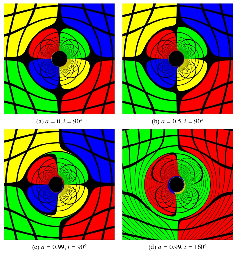
This stage applies to the rendered images only. The renders in Figure 1 place the observer at  with
 . The quantitative results are not read off a camera image: the boundary solver below works directly in the launch angles
 at the same robs, so no reported value of
 ,
 , or any fitted exponent depends on a field-of-view choice.
For an image of height  and width
 , the renderer converted each pixel
 to centered screen coordinates
 and
 , and then to normalized camera-plane coordinates
where  are the horizontal and vertical fields of view. With d the black-hole direction in camera coordinates and
 the local orthonormal screen basis around it, the unit ray vector for the pixel was
For the centered renders, the camera axes point right, down, and toward the black hole, respectively, so  ,
 , and
 .
The two launch angles used by the tracer were then
The angle  is the screen azimuth, and is referred to by that name throughout the sections that follow. The observer inclination
 is the polar angle between the black-hole spin axis and the observer’s line of sight, so
 and
 are pole-on views and
 is edge-on. For the symmetric Kerr setup, the asymmetric quantities are invariant under
 , so the quantitative plots use
 . The launch angles set the initial photon momentum through the celestial coordinates
 of Bardeen27, which are the impact parameters of the ray on the sky of an observer at infinity. The tracer evaluates them at the finite observer radius rather than transforming a local four-momentum through an observer tetrad, and no momentum component is recomputed afterwards. Writing
 for the magnitude of the impact parameter,
where  and
 . The factor
 corrects the flat-space impact parameter
 for the finite observer radius and tends to unity as
 , while the minus signs follow from
 pointing down the screen, so that screen-up corresponds to
 . With the affine normalization
 , the constants of motion are
 and
 , and the polar momentum follows from the Carter relation evaluated at the observer,
 , with its sign following
 ,
Rays are traced backwards from the camera, so the photon is initially ingoing and  is the negative root of the null condition
 ,
Ray tracing and outcome classification
For each screen direction , the tracer launched one ray and evolved its photon trajectory using first-order Hamiltonian geodesic equations. The constants of motion follow the standard Kerr geodesic treatment of Chandrasekhar and Bardeen25,27. With  and
 held fixed, the tracer evolved the reduced state
initialized as above, so that the initial trajectory was null.1 The equations integrated by the tracer had the Hamiltonian form
where  is an affine parameter. In practice, the tracer needed only the equations for
 , and
 to determine whether the ray escaped or was captured and, for escaping rays, its final direction.
The Kerr tracer used an adaptive Dormand–Prince fourth/fifth-order Runge–Kutta stepper. The integrator stopped when the ray reached an inner capture radius just outside the outer horizon,  , or when it reached an outer escape radius of
 . The tracer classified a ray that crossed the inner radius as captured, and a ray that reached the outer radius as escaped. The implementation traced these ODEs in batches over the image grid, using the pixel-to-angle map to supply for each ray. For , the maximum affine parameter was
 , with a safety limit of 200,000 attempted integration steps per ray.
The capture surface  is valid only if it lies inside every photon turning point an escaping ray can reach. The innermost is the prograde equatorial photon orbit
 , which bounds the radii of all spherical photon orbits from below, so
 suffices at every inclination. This holds for
 : at
 the capture surface would lie
 outside
 , and rays turning between the two would be misrecorded as captured. The sweep is therefore truncated at
 , where
 remains inside
 . Lowering the cut to
 shifts every fitted exponent below by less than
 , so the reported scalings do not depend on where the sweep is stopped.
For lensing visualization, the renderer colored each captured ray black and mapped each escaped ray onto a point on a sphere. For each escaped ray, the tracer recorded the final deflection angle after escape. The renderer then combined that deflection angle with the screen azimuth to assign a source direction  , converted it to the screen-aligned angular coordinates
 and
 , wrapped both coordinates over
 , and divided them into
 and
 horizontal and vertical periods respectively. If the wrapped phase fell within the stripe width—
 of the corresponding angular period—the renderer colored the pixel black. Otherwise it colored the pixel by the quadrant of the sphere in which the deflection angle landed. The renders in Figure 1 used
 , so each period spans
 with the stripe occupying its central . These are cosmetic choices. No quantitative result is read off these images.
Shadow-boundary extraction
The tracer sweeps over the observer launch angles to try to find  —the angle at which the transition of a ray between captured and escape happens—using the captured/escaped classifier. Launch angles inside
 are captured directions. All others escape. For each fixed screen azimuth, the tracer treated the classifier
 as a two-valued function returning either captured or escaped, and solved for
The infimum captures the first escaped ray as  sweeps through the range. This notation assumes a single captured-to-escaped transition within the bracket. Iterative bracketing found the numerical value. Given a current bracket
 , the midpoint was
where  is a predetermined tolerance value. The tracer repeated this search over a sweep of and cached the result for the asymmetry calculations. The renderer produced the representative shadow images at
 pixels. The quantitative boundary measurements do not come from those pixels. They come directly from angular boundary solves. The main parameter run placed the observer at and sampled 1041 spins and 111 inclinations, giving
 configurations. Spin was stepped from by
 up to
 (91 values), then refined a hundredfold to
 between and (950 values), where both observables vary most rapidly. Inclination was stepped from by
 to
 (88 values), then refined tenfold to
 out to
 (23 values). The boundary search used 97 initial bracket samples,
 rad, at most 96 bisection iterations, 361 azimuth samples for extremum searches, five refinement levels, and 721 full-boundary samples for the circularity calculation. The Kerr ray integrator used relative and absolute tolerances of
 and
 , respectively, with stricter and
 tolerances on axis-refined rays. A convergence check at compared these settings with an ultra-accurate run using 129 bracket samples,
 , 721 extremum-search azimuth samples, six refinement levels, and 1081 full-boundary samples. Across the common spin samples, the maximum absolute changes were less than
 for and less than
 for , showing that the reported trends are stable under further refinement. Because and are fixed in the reduced system,
 and
 are conserved by construction. We checked representative captured and escaped Kerr rays throughout their integration and found maximum dimensionless null-constraint and relative Carter-constant residuals of
 and
 , respectively, at the production tolerances. Tightening both tolerances by a factor of 100 reduced these maxima to
 and
 , confirming that the conserved quantities remain numerically stable .11 × 10−9 and 2.06 × 10⁻⁹, confirming that the conserved quantities remain numerically stable29,30.
The boundary solver was checked against the one case with a closed-form answer. At the shadow is the circle of radius . The check re-solves that boundary by direct bisection on traced rays rather than reading the tabulated entry, which for a spherically symmetric metric returns the closed-form of Eq. (2) without tracing a ray and so cannot test the integrator. At the main-run sampling settings the recovered angle gives  from the Schwarzschild orbit-equation integrator and a mean
 over 361 azimuths from the Kerr integrator at , against the exact
 : relative deviations of
 and at most
 , with the boundary circular to
 . Tightening from to
 changes by less than
 , so the residual reflects the ray integrator rather than the bracketing resolution.
The same check extends to against the analytic Kerr critical curve. With , each boundary point’s and  follow from its above, and the ray is critical only if that pair lies on the spherical-photon-orbit locus27; solving
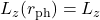 and comparing the predicted tests each sample against the curve pointwise. Over six configurations spanning
 —
 and —
 , all 721 samples of each matched to a median
 and a maximum
 in (Figure 2), the same order as the residual above.
Projection of the boundary onto the observer screen
Once the solver had , it mapped each boundary point to tangent-plane screen coordinates. Defining
the screen coordinates were
The extracted shadow boundary is thus a discrete set of points
All later measurements use this representation.
Asymmetry measurements
The boundary-analysis step approximated two shadow-shape quantities from the extracted boundary. First, the left and right critical directions define the horizontal tangent ratio:
Here “right” and “left” are the horizontal screen directions  and
 , i.e.
 in Eq. (18). Since
 , the right-hand point is the prograde side for
 and the left-hand point the retrograde side. This ratio provides the direct boundary measurement used later to define the left–right asymmetry observable . Both tangents in Eq. (20) are measured from the screen origin, not from the fitted circle centre. Writing the side extents as
 and
 , with
 and
 measured from the fitted centre, shows that
 responds to a sideways shift of the whole image as well as to a genuine difference between the extents. The Results separate the two.
To quantify the shadow’s departure from a perfect circle, the analysis also compared the boundary with a fitted circle. This is the global algebraic least-squares circle through all 721 boundary samples. If  is the boundary radius measured from the fitted center, then the mean radius is
The circularity-deviation amplitude is then
and the corresponding circularity deviation is
Unlike , this quantity measures radial departure from a fitted circle rather than left–right displacement alone.
Two further quantities separate the displacement of the shadow from its shape. The first is the horizontal offset of the fitted centre, normalized by the mean radius,
where  is the fitted circle centre; the vertical offset
 is defined in the same way and must vanish for the symmetric configuration considered here. The second quantity is a reflection asymmetry measured about the fitted centre, so it is blind to displacement by construction. With
the reflection amplitude and its normalized form are
The normalization is that of Eq. (23), so both read on the same scale. The integral is evaluated on a uniform grid of  azimuths about the fitted centre. Varying that number between
 and
 changes
 by less than
 relative. Replacing
 with
 gives the top–bottom counterpart
 , used below as a control that must vanish.
Together, and describe the shape of the boundary about its own centre, while  measures the displacement of that centre. The measure mixes the two.
Results and Discussion
The generated shadows show two main geometric effects of rotation: left–right asymmetry and deformation of the overall shadow8,11,26,9. To study these separately, the analysis uses two extracted shape quantities: , which measures deformation, and , which measures left–right asymmetry. Two further quantities, the centre displacement of Eq. (24) and the reflection asymmetry of Eq. (26), are carried through the same analysis. They are what separates the roles of and . The quantity is used instead of the raw because it is easier to interpret together with :
and are consistent with each other: both equal when there is perfect symmetry and grow when the asymmetry becomes stronger.
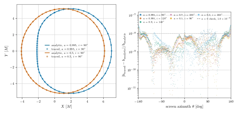 , and
 . Right: fractional deviation of each sample from the curve for six
 configurations; all 4326 fall below , comparable to the check (dashed).
Before the quantitative analysis, Figure 1 gives a qualitative overview: increasing spin transforms the dark central region from a near-symmetric disk into a visibly distorted one. The stripe patterns show how strongly nearby light rays are deflected around the black hole. The Schwarzschild image is the symmetric baseline. At moderate spin, a slight but noticeable asymmetry is visible. At high spin, the dark central region visibly becomes strongly deformed and asymmetrical31,32. The nested stripe bands near the edge of the dark region are higher-order lensed images of the same pattern, formed by rays that wind one or more times around the black hole before escaping—the photon-ring structure7,33,34,35, indicated qualitatively rather than resolved order by order.
The same pattern is observed in the dataset. Both and are in the non-rotating case and increase when spin increases. The values are exactly zero by construction rather than by measurement: for a spherically symmetric metric the boundary routine returns the closed-form of Eq. (2) at every azimuth, so the extracted boundary is an exact circle. The traced boundary is quantified in the validation above. The maximum values of both quantities ( and
 ) occur at the highest sampled spin, at . For scale, is normalized as the circularity deviation reported for M87*, and the grid maximum falls below the
 that the 2017 image permits19, though that bound is set on the emission ring rather than the shadow boundary. Its onset—negligible until spin nears extremality, strongest at —follows the trend found for the Hioki–Maeda distortion parameter8.
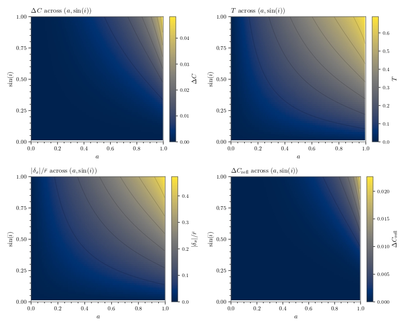 (top left) and (top right) over the sampled
 grid. Both rise smoothly with spin and with , so shadow morphology is set jointly by spin and viewing geometry, not by spin alone. The bottom row shows the centre displacement
 (left) and the reflection asymmetry (right) on the same grid. The displacement map resembles that of , while the reflection map resembles that of but is steeper still.
The same structure is shown in Figure 3. The dependence of both observables on spin and is smooth and coherent, suggesting that shadow deformation may be describable with relatively simple empirical laws.
The maps also make it clear that spin alone does not determine the observed shadow shape. Inclination plays an important role in deciding how strongly rotational effects appear in the image plane. A highly rotating black hole does not necessarily produce a strongly deformed shadow in every viewing configuration.
Although global maps are useful, one-dimensional slices are better for showing how the observables grow. Figure 4 shows the dependence on spin at fixed inclination.
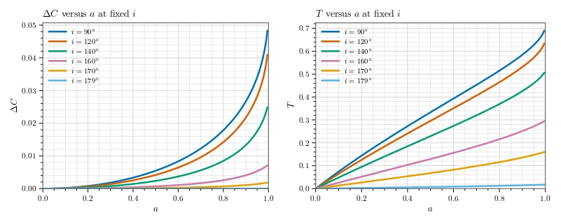 (left) and (right) versus spin at
 and
 . rises smoothly from low spin, while stays small until nears , then climbs steeply
Figure 4 shows one of the clearest differences between and . At low and moderate spin, rises smoothly and steadily, while stays relatively small. Only as spin approaches does rise much more strongly than . The natural reading of this, that the shadow becomes noticeably asymmetric before it becomes noticeably deformed, does not survive a closer look at what measures.
Because Eq. (20) is referenced to the screen origin, responds to the displacement  of the shadow as well as to its shape. Two knockout tests at , , where
 , separate them: forcing
 while keeping the measured displacement gives
 , and setting
 while keeping the measured difference between the extents gives
 . The two do not sum to the measured value, since is a ratio, but they locate the effect unambiguously. The clearest single case is
 , , where the extents measured from the fitted centre differ by 0.06% (
 ,
 ) yet
 , because
 .
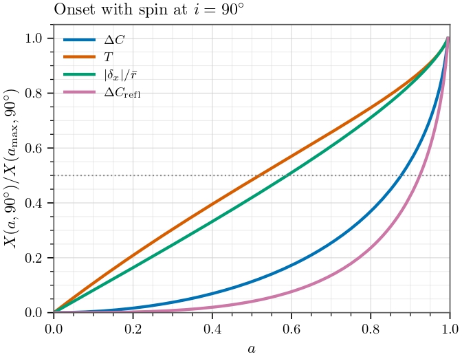 divided by its own value at the highest sampled spin, against . The centre displacement tracks closely and both rise early, while and the reflection asymmetry rise late. The dotted line marks half of each maximum.
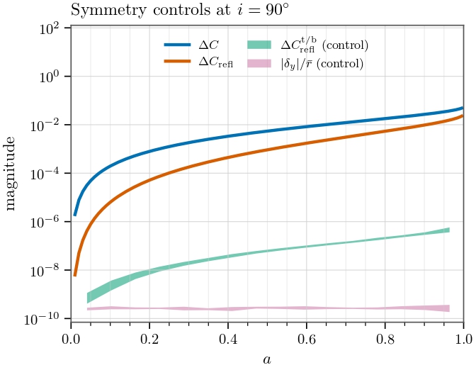 against the two controls that must vanish, on a logarithmic scale. The controls stay below
 while the measures they mirror grow past
 . Bands span the range within each spin bin, so their width is round-off scatter, not spin dependence.
Figure 5 compares the four measures on a common scale, each divided by its own edge-on value at . The displacement tracks closely and both rise early, reaching half of their maximum at  and
 , while the two shape measures rise late, at
 for and
 for . The ordering is the opposite of the one the raw curve suggests: what appears early with spin is the displacement, and the reflection asymmetry of the outline is the last of the four to respond.
This does not make the deformation an artifact:  and
 at the highest sampled spin are real, and the displacement is frame dragging rather than a numerical effect. The separation between asymmetry and deformation must simply be drawn between on one side and and on the other, rather than between and .
and are still not two ways of measuring the same thing. The difference is not the one it appears to be: responds to spin sooner because the shadow shifts sideways before its outline changes shape, not because asymmetry precedes deformation.
Two controls confirm that the measured asymmetries are not artifacts of the boundary extraction. Each mirrors a genuine measure across an axis of symmetry, so each must vanish. Across all 115,551 configurations  stays below
 and below
 , against maxima of
 and
 for the left–right measures they mirror (Figure 6).
The observables are also dependent on the observer’s inclination at fixed spin. This shows how strongly rotational effects are projected into the observer’s image.
The inclination slice shows that both and are suppressed when the observer moves closer to the rotating poles. So high-spin shadow can appear much more symmetrical and less distorted near the spin axis.
Figure 7 and the numerical samples make this pattern clearer and more concrete. Even at extremely high spin, both and reduce substantially as the viewing configuration becomes less favorable. At , decreases from about  at
 to
 at
 ,
 at
 ,
 at ,
 at
 , and only about
 at . Over the same range, decreases from about
 at to
 at ,
 at ,
 at ,
 at , and only about
 at . This result suggests observer inclination as one of the most important controls of the observed shadow shape.
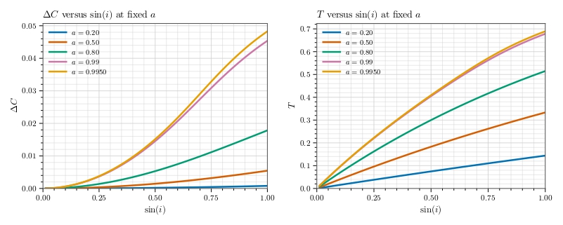 (left) and (right) versus at
 and . Both fall steeply toward pole-on viewing, and the two highest-spin curves nearly coincide.
To establish a more rigorous view of how the observables “grow” with and in the slice plots, we examine the gradient of and with respect to and . The gradients were computed with second order finite differences on the sampled  grid, including second order boundary estimates, and plotted as the magnitude
 . It shows where and are most sensitive to parameter changes.
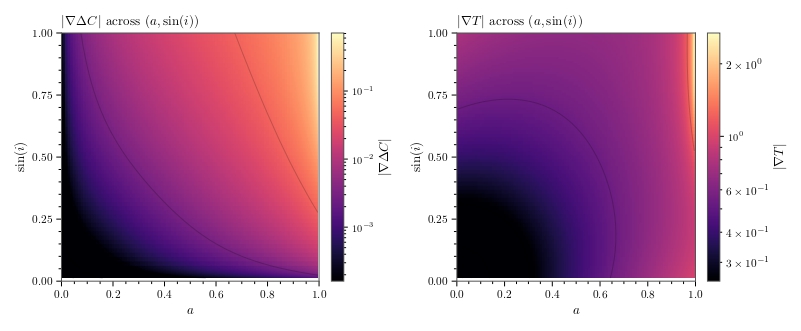
 for (left) and (right), on a logarithmic color scale. responds across the whole grid, while is sensitive mainly where and both approach .
Figure 8 shows that responds more steadily and broadly across the parameter grid but still becomes more sensitive when and grow, especially when they both approach . The gradient magnitude of , by contrast, grows rapidly only as and approach . In other words, left–right asymmetry is a broad response observable, while strong deformation becomes especially sensitive at high spin.
The numerical sample shows the same picture. The median value of  is about
 , while the median value of
 is about
 . The maximum of is about
 , and the maximum of reaches about
 . For inclination dependence, the median
 is about
 , while the median
 is about
 . This indicates that varies substantially over a broad region, while rises much more sharply when approaches .
From another perspective, the slice plots of and , at fixed inclinations, have similar shapes as a function of . Similarly, at fixed spin, the slice plots have similar shapes. This behavior may imply that the dependencies of the observables are not strongly entangled. This behavior is expected if the observables can be approximated as
A second indication is that if  is approximately separable, then
 should depend mainly on . In Figure 9, this is exactly what is seen: for fixed inclination, the spread of
 remains small, with median standard deviations of about
 for and
 for , and maximum standard deviations of only about
 and , respectively. This indicates that after normalization by a reference inclination, the remaining spin dependence is weak, and the curves approximately collapse.
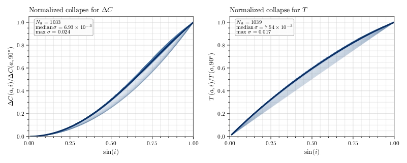 for (left) and (right), restricted to
 and
 . Curves at different spins overlap closely, supporting
 .
This structure is inherited from the analytic critical curve. In Bardeen’s parametrization27 the boundary is traced by the spherical photon radius  through
 and
 , so spin enters through
 and
 while inclination enters through the projection, the two mixing only via the
 term. Approximate separability is therefore expected, with the violation smallest near , where the collapse in Figure 9 is tightest.
The approximate product structure suggested by the slice plots and normalized collapse can be tested quantitatively through regression. Using a multiplicative power-law model (consistent with the above form), the fitted regression laws are
Fitting the same model to the two additional measures places them on either side of this split (Table 1): the exponents of agree with those of to within  , both close to , while and are steeper in by factors of
 and
 . The regression thus reproduces, in the exponents alone, the ordering of Figure 5.
Table 1 | Power-law fits  for all four measures, from ordinary least squares on the log-transformed variables over the 115,440 grid points with .
 is computed in the log space where the residuals are minimized.
 |  |  |  | |
| | 0.04326 | 2.4321 | 1.9420 | 0.9969 |
| | 0.70902 | 1.0294 | 0.9128 | 0.9981 |
| 0.46312 | 1.0986 | 0.9875 | 0.9994 |
| | 0.019808 | 3.5060 | 2.8702 | 0.9943 |
As an important note, these regression results should not be treated as exact analytic relations but empirical summaries of the sample grid. Their residual behavior is assessed in Figure 10. Both the regression results, especially for , follow the measured values closely, with coefficients of determination  and
 for and , respectively. The fit was ordinary least squares on the log-transformed variables, a linear regression of
 and
 on
 and
 over the 115,440 grid points with . The
 values quoted above are linear-space. In the log space where the residuals are minimized they are
 and
 . Standard errors from the same fit give 95% intervals
 ,
 for and
 ,
 for . These are nominal: the grid is deterministic and the residuals are systematic, and refitting to
 shifts for by
 , some four times its interval width, so they bound the uncertainty from below. The validation panel reinforces this result, especially for , where the points cluster tightly around the one-to-one reference line.
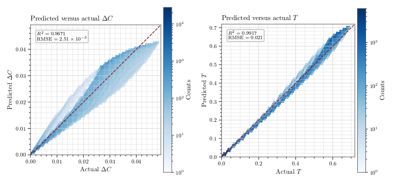 (left) and (right), as hexagonal-bin densities with the one-to-one line dashed. The density hugs the line, while the density is a wider lens that broadens toward large .
These regression results are also consistent with the earlier discussed trends. For , the exponents of both and are close to , indicating that grows approximately linearly with both parameters. For , the exponents of both and are higher, indicating that becomes much more sensitive when the parameter grows larger.
All together, the visual images, extracted observables, slice plots, derivative analysis and regression result support one consistent physical interpretation: Spin-induced shadow changes occur in layers. The sideways displacement of the shadow appears early and grows steadily, while deformation of its outline appears later and grows faster. The strength of these deforming effects is projected to the observer’s view by the observer’s inclination. The observed shadow distortion is therefore controlled by the combination of spin and projection.
A few limitations should be stated briefly. The regression result and the product structure are empirical approximations, not analytic formulas derived from the metric. The calculation of the derivatives near the symmetric limits is unstable because the observables become extremely small, so the iterative bracketing and floating-point operations become inaccurate. Finally, this analysis focuses on shadow geometry rather than full observational image reconstruction.
The near-extremal regime is the delicate one. The observables stiffen there—at ,  rises from
 at to
 at , which is why the spin step is refined a hundredfold above —while the margin
 that keeps the capture test sound falls from
 at to
 at
 before changing sign. A stopping surface fixed as a fraction of
 therefore cannot be pushed to extremality in principle. Doing so would require tying it to itself. The results should not be extrapolated past .
Conclusion
This paper developed a computational framework and analyzed black hole shadow deformation, using the Schwarzschild metric as a baseline and introducing rotation with the Kerr metric. Spin introduces distortion in the form of left–right asymmetry and overall shadow deformation. The results indicate that the displacement of the shadow centre, , appears earlier and grows more steadily with spin, while deformation of the outline, measured by and , becomes apparent only near extremal spin. The left–right measure follows the displacement rather than the shape, which is why it appears to respond first.
Beyond the visual image, the extracted measurements, derivative maps, and regression fits showed that the dependence of and on spin and inclination is smooth, interpretable, and approximately separable. The fitted power law, though not an exact analytic derivation, captured the overall trends well. These results further reinforce the role of simplified and isolated computational studies as a bridge between relativistic theory and observable image distortion1,16.
Future extensions could add a more realistic emission environment or additional spacetime parameters36,37,38,39. This research clarifies how rotation affects black hole shadows and establishes a foundation for more advanced studies.
Acknowledgements
The author thanks Richard Stiskalek for his guidance and mentorship throughout this project.
- For example, a 4000 × 4000 image with a 40o field of view maps pixel (1800, 2200) at a = 0.9, i = 90o, M = 1, and robs = 100M to α = 0.0514277771, θ = 2.3561944902, and (E, Lz, Q, pr , pθ ) = (1, 3.6716418834, 13.4809541196, −1.0190103515, 3.6716418834), with initial null residual |gμν pμ pν | = 6.6 × 10⁻¹⁷. ↩︎
References
- H. Falcke, F. Melia, E. Agol. Viewing the shadow of the black hole at the Galactic center. Astrophysical Journal Letters. Vol. 528, pg. L13–L16, 2000, https://doi.org/10.1086/312423. [↩] [↩] [↩]
- T. Johannsen, D. Psaltis. Testing the no-hair theorem with observations in the electromagnetic spectrum. Astrophysical Journal. Vol. 718, pg. 446–454, 2010, https://doi.org/10.1088/0004-637X/718/1/446. [↩]
- D. Psaltis, F. Özel, C.-K. Chan, D. P. Marrone. A general relativistic null hypothesis test with Event Horizon Telescope observations of the black hole shadow in Sgr A. Astrophysical Journal. Vol. 814, pg. 115, 2015, https://doi.org/10.1088/0004-637X/814/2/115. [↩]
- M. Mars, C. F. Paganini, M. A. Oancea. The fingerprints of black holes—shadows and their degeneracies. Classical and Quantum Gravity. Vol. 35, pg. 025005, 2018, https://doi.org/10.1088/1361-6382/aa97ff. [↩]
- A. Grenzebach, V. Perlick, C. Lämmerzahl. Photon regions and shadows of Kerr–Newman–NUT black holes with a cosmological constant. Physical Review D. Vol. 89, pg. 124004, 2014, https://doi.org/10.1103/PhysRevD.89.124004. [↩] [↩] [↩]
- P. V. P. Cunha, C. A. R. Herdeiro, E. Radu. Fundamental photon orbits: black hole shadows and spacetime instabilities. Physical Review D. Vol. 96, pg. 024039, 2017, https://doi.org/10.1103/PhysRevD.96.024039. [↩] [↩]
- S. E. Gralla, D. E. Holz, R. M. Wald. Black hole shadows, photon rings, and lensing rings. Physical Review D. Vol. 100, pg. 024018, 2019, https://doi.org/10.1103/PhysRevD.100.024018. [↩] [↩]
- K. Hioki, K. Maeda. Measurement of the Kerr spin parameter by observation of a compact object’s shadow. Physical Review D. Vol. 80, pg. 024042, 2009, https://doi.org/10.1103/PhysRevD.80.024042. [↩] [↩] [↩] [↩]
- T. Johannsen. Photon rings around Kerr and Kerr-like black holes. Astrophysical Journal. Vol. 777, pg. 170, 2013, https://doi.org/10.1088/0004-637X/777/2/170. [↩] [↩]
- O. Yu. Tsupko. Analytical calculation of black hole spin using deformation of the shadow. Physical Review D. Vol. 95, pg. 104058, 2017, https://doi.org/10.1103/PhysRevD.95.104058. [↩]
- A. A. Abdujabbarov, L. Rezzolla, B. J. Ahmedov. A coordinate-independent characterization of a black hole shadow. Monthly Notices of the Royal Astronomical Society. Vol. 454, pg. 2423–2435, 2015, https://doi.org/10.1093/mnras/stv2079. [↩] [↩]
- Event Horizon Telescope Collaboration. First M87 Event Horizon Telescope results. I. The shadow of the supermassive black hole. Astrophysical Journal Letters. Vol. 875, pg. L1, 2019, https://doi.org/10.3847/2041-8213/ab0ec7. [↩]
- R.-S. Lu, A. E. Broderick, F. Baron, J. D. Monnier, V. L. Fish, S. S. Doeleman, V. Pankratius. Imaging the supermassive black hole shadow and jet base of M87 with the Event Horizon Telescope. Astrophysical Journal. Vol. 788, pg. 120, 2014, https://doi.org/10.1088/0004-637X/788/2/120. [↩]
- Event Horizon Telescope Collaboration. First M87 Event Horizon Telescope results. IV. Imaging the central supermassive black hole. Astrophysical Journal Letters. Vol. 875, pg. L4, 2019, https://doi.org/10.3847/2041-8213/ab0e85. [↩]
- Event Horizon Telescope Collaboration. First Sagittarius A Event Horizon Telescope results. I. The shadow of the supermassive black hole in the center of the Milky Way. Astrophysical Journal Letters. Vol. 930, pg. L12, 2022, https://doi.org/10.3847/2041-8213/ac6674. [↩]
- Y. Mizuno, Z. Younsi, C. M. Fromm, O. Porth, M. De Laurentis, H. Olivares, H. Falcke, M. Kramer, L. Rezzolla. The current ability to test theories of gravity with black hole shadows. Nature Astronomy. Vol. 2, pg. 585–590, 2018, https://doi.org/10.1038/s41550-018-0449-5. [↩] [↩]
- Event Horizon Telescope Collaboration. First M87 Event Horizon Telescope results. V. Physical origin of the asymmetric ring. Astrophysical Journal Letters. Vol. 875, pg. L5, 2019, https://doi.org/10.3847/2041-8213/ab0f43. [↩]
- Z. Younsi, D. Psaltis, F. Özel. Black hole images as tests of general relativity: effects of spacetime geometry. Astrophysical Journal. Vol. 942, pg. 47, 2023, https://doi.org/10.3847/1538-4357/aca58a. [↩]
- Event Horizon Telescope Collaboration. First M87 Event Horizon Telescope results. VI. The shadow and mass of the central black hole. Astrophysical Journal Letters. Vol. 875, pg. L6, 2019, https://doi.org/10.3847/2041-8213/ab1141. [↩] [↩]
- Event Horizon Telescope Collaboration. First Sagittarius A* Event Horizon Telescope results. VI. Testing the black hole metric. Astrophysical Journal Letters. Vol. 930, pg. L17, 2022, https://doi.org/10.3847/2041-8213/ac6756. [↩]
- D. Psaltis, L. Medeiros, P. Christian, F. Özel, Event Horizon Telescope Collaboration. Gravitational test beyond the first post-Newtonian order with the shadow of the M87 black hole. Physical Review Letters. Vol. 125, pg. 141104, 2020, https://doi.org/10.1103/PhysRevLett.125.141104. [↩]
- P. Kocherlakota, L. Rezzolla, H. Falcke, C. M. Fromm, M. Kramer, Y. Mizuno, A. Nathanail, H. Olivares, Z. Younsi, Event Horizon Telescope Collaboration. Constraints on black-hole charges with the 2017 EHT observations of M87*. Physical Review D. Vol. 103, pg. 104047, 2021, https://doi.org/10.1103/PhysRevD.103.104047. [↩]
- C. W. Misner, K. S. Thorne, J. A. Wheeler. Gravitation. W. H. Freeman, 1973. [↩]
- R. M. Wald. General relativity. University of Chicago Press, 1984. [↩] [↩]
- S. Chandrasekhar. The mathematical theory of black holes. Oxford University Press, 1983. [↩] [↩]
- L. Medeiros, D. Psaltis, F. Özel. A parametric model for the shapes of black hole shadows in non-Kerr spacetimes. Astrophysical Journal. Vol. 896, pg. 7, 2020, https://doi.org/10.3847/1538-4357/ab8bd1. [↩] [↩]
- J. M. Bardeen. Timelike and null geodesics in the Kerr metric. in Black holes (eds C. DeWitt & B. S. DeWitt) pg. 215–239, Gordon and Breach, 1973. [↩] [↩] [↩] [↩] [↩]
- S. E. Gralla, A. Lupsasca. Observable shape of black hole photon rings. Physical Review D. Vol. 102, pg. 124003, 2020, https://doi.org/10.1103/PhysRevD.102.124003. [↩]
- T. Bronzwaer, J. Davelaar, Z. Younsi, M. Mościbrodzka, H. Falcke, M. Kramer, L. Rezzolla. RAPTOR I: time-dependent radiative transfer in arbitrary spacetimes. Astronomy and Astrophysics. Vol. 613, pg. A2, 2018, https://doi.org/10.1051/0004-6361/201732149. [↩]
- J. M. Velásquez-Cadavid, J. A. Arrieta-Villamizar, F. D. Lora-Clavijo, O. M. Pimentel, J. E. Osorio Vargas. OSIRIS: a new code for ray tracing around compact objects. European Physical Journal C. Vol. 82, pg. 103, 2022, https://doi.org/10.1140/epjc/s10052-022-10054-0. [↩]
- S. E. Gralla, A. Lupsasca, A. Strominger. Observational signature of high spin at the Event Horizon Telescope. Monthly Notices of the Royal Astronomical Society. Vol. 475, pg. 3829–3853, 2018, https://doi.org/10.1093/mnras/sty039. [↩]
- A. Lupsasca, A. P. Porfyriadis, Y. Shi. Critical emission from a high-spin black hole. Physical Review D. Vol. 97, pg. 064017, 2018, https://doi.org/10.1103/PhysRevD.97.064017. [↩]
- M. D. Johnson, A. Lupsasca, A. Strominger, G. N. Wong, S. Hadar, D. Kapec, R. Narayan, A. Chael, C. F. Gammie, P. Galison, D. C. M. Palumbo, S. S. Doeleman, L. Blackburn, M. Wielgus, D. W. Pesce, J. R. Farah, J. M. Moran. Universal interferometric signatures of a black hole’s photon ring. Science Advances. Vol. 6, pg. eaaz1310, 2020, https://doi.org/10.1126/sciadv.aaz1310. [↩]
- H. Paugnat, A. Lupsasca, F. H. Vincent, M. Wielgus. Photon ring test of the Kerr hypothesis: variation in the ring shape. Astronomy and Astrophysics. Vol. 668, pg. A11, 2022, https://doi.org/10.1051/0004-6361/202244216. [↩]
- A. Cárdenas-Avendaño, A. Lupsasca. Prediction for the interferometric shape of the first black hole photon ring. Physical Review D. Vol. 108, pg. 064043, 2023, https://doi.org/10.1103/PhysRevD.108.064043. [↩]
- Z. Gelles, E. Himwich, M. D. Johnson, D. C. M. Palumbo. Polarized image of equatorial emission in the Kerr geometry. Physical Review D. Vol. 104, pg. 044060, 2021, https://doi.org/10.1103/PhysRevD.104.044060. [↩]
- G. N. Wong. Black hole glimmer signatures of mass, spin, and inclination. Astrophysical Journal. Vol. 909, pg. 217, 2021, https://doi.org/10.3847/1538-4357/abdd2d. [↩]
- S. Hadar, M. D. Johnson, A. Lupsasca, G. N. Wong. Photon ring autocorrelations. Physical Review D. Vol. 103, pg. 104038, 2021, https://doi.org/10.1103/PhysRevD.103.104038. [↩]
- E. Himwich, M. D. Johnson, A. Lupsasca, A. Strominger. Universal polarimetric signatures of the black hole photon ring. Physical Review D. Vol. 101, pg. 084020, 2020, https://doi.org/10.1103/PhysRevD.101.084020. [↩]