Lap-by-Lap Machine Learning Prediction of End-of-Race Formula 1 Points from Lap-Level Timing and Telemetry Data 

Abstract

This paper uses per-lap regression to predict each driver’s Formula 1 finishing points from every lap of a race starting at the fourth lap (at the earliest). The dataset covers 171 races from 2018 to 2025, with telemetry aggregated to the second. Timing, tire data, weather, and circuit data are aggregated to roughly 175,000 total laps across the drivers. Four tree ensemble models were tuned by grid search and evaluated under expanding-window cross-validation on the 2021 – 2024 seasons, with 2025 held out for testing. XGBoost performed best, reaching an R² of 0.793 and a mean absolute error of 1.98 on the held-out 2025 season, with all four models finishing within 0.013 R² of each other. We conducted an ablation study, which shows that the current race position carries the most predictive signal, since removing it drops R² from 0.79 to 0.418, while timing and tire information is the largest other feature group with a measurable cost. Telemetry, circuit, and driver identity features show no detectable effect. Prediction error also falls steadily as a race progresses, from around two and a half points in the opening stages to near one point by the end. These results show that accurate live in-race prediction is possible, and that performance is limited by the information that is given to the model more than the choice of the model. 

Keywords: Formula 1, machine learning, race prediction, telemetry, XGBoost, regression, motorsport analytics

Introduction

Formula 1 is the highest class of international single-seater motorsport. Originating in 1950 with the first World Drivers’ Championship, it has since grown into a global sport followed by hundreds of millions of viewers. It has reached a cumulative global television audience of roughly 1.9 billion across the 2019 season¹. Components of the races are shaped long before the cars reach the grid, in factories where aerodynamics and other key components are developed². Race outcomes also support a large betting market. Horse betting prices are known to be imperfect³, and in sports betting in general, machine learning models can bet profitably⁴.

Race results are dependent on many factors including car performance, driver skill, tire management, pit strategy, weather, safety car periods, and the pace and strategy of rivals. Work that tries to separate the contribution of the driver from that of the car has found that a small number of drivers perform above the level of their equipment⁵, while the car explains far more of the variation in race results than the driver does^6,7. 

For the teams, good forecasting has a direct competitive value. Race engineers make important decisions under time pressure, such as deciding when to pit and which tire compound to fit. They also make split second decisions, such as how to respond to varied conditions such as safety cars. Models that anticipate how a race will develop, in Formula 1 and circuit motorsport more broadly, allow strategists to prepare these decisions in advance and react to events during the race with quantitative support, extending beyond fixed simulations or instinct^8,9,10,11. 

Still, Formula 1 results are hard to predict, and much of that difficulty cannot be removed. Races are interrupted by rare events with large effects. Some examples are mechanical failures that end a leading car’s race, a first lap collision, sudden rain, or a safety car that slows the whole field and removes a gap that a driver has spent building. These events break the relationship between mid-race pace and final result that a model would otherwise use, and they are difficult to anticipate. They are hard enough to predict that machine learning has been used to predict whether a race will produce accidents at all¹². Retirements in particular are known to be hard to handle, and earlier work has set them aside⁵. 

Machine learning is well suited to this problem because of how it can learn complex, non-linear relationships between many variables without being told the form of these relationships in advance. Classical statistical methods struggle with the high dimensionality and the many interactions in race data, while modern learning methods tend to handle structured, tabular data of this type well. Outcome prediction with such methods is well established across other sports^13,14. Modern learning methods have already been applied to Formula 1 problems, including embedding-based deep networks⁸, reinforcement learning⁹, ensemble tree models¹⁵, graph neural networks¹⁶, and genetic algorithms for strategy optimization¹⁷. Some of this work now targets the finishing result directly¹⁸. 

The data available has also become more detailed. Prior work relied on season-level summaries², but lap-level timing data makes it possible to model a race lap by lap as it develops, rather than as a single fixed snapshot^8,19,20. This data is now openly accessible through tools such as the FastF1 API²¹. Recent work uses lap by lap resolution to forecast how rank positions change over the following laps in other racing series²², to predict when a driver will pit from FastF1 timing data²³. At an even finer resolution, one study forecasts tire energy within a race from a team’s own proprietary telemetry²⁴. It also lets us ask how confident a model is at each point in the race, and where that confidence is wrong. This is a question that parallels in-play win-probability prediction in other sports^25,26.

The aim of this work is to build and carefully evaluate a system that predicts the championship points a driver will score in a given race from lap-level telemetry and to describe where and why the system fails. 

Relevant Works

Machine learning outcome prediction has been demonstrated in soccer^27,28 and basketball²⁹. Tennis forecasting has been benchmarked across regression, point based, and paired comparison models, including Elo³⁰. Boosting ranking models have predicted road cycling outcomes³¹. In Formula 1, Patil et al.² carried out a data driven analysis to find which factors most affect total points that a driver scores across a season. They describe it as the first study of its kind for Formula 1. Patil et al.² used five seasons of data (2015 – 2019) and twenty one variables. The study has three main limitations: it predicts the championship result, rather than specific individual races; it relies only on a linear regression; and it covers only five seasons of data, all from before the 2022 regulation change, so its findings may not hold under later rulesets.

The Deep-Racing study⁸ introduced an Embedded Deep Neural Network (EDNN) to predict winning strategy and each driver’s rank lap by lap. It used data from 2015 to 2022 from the Ergast API. The model predicted a driver’s rank on upcoming laps with a test RMSE of about two places (R² of 0.39). Its main limitation is that it splits the problem across two networks. One is for driver rank with the other for the pit stop lap. These two are evaluated separately. 

Another study⁵ worked in the opposite direction and tried to separate the effect of the driver from the effect of the car using a time-rank duality. Combining a regression on the 2022 season with betting odds for the 2023 Qatar Grand Prix, it found that Max Verstappen and Fernando Alonso both performed above the level of their cars. The approach is not based on machine learning and it is aimed at attribution, not forecasting race outcomes. Its biggest limitation is retirements (DNFs) are not modeled, with their inclusion left as future work.

Another study by Thomas et al.⁹ used explainable reinforcement learning to optimize pit strategy. Its state space includes track, race progress, current position, tire compound and degradation, the gaps to the cars ahead and behind and to the leader, and safety car status. For our purposes, the main limitation is that it optimizes finishing position through strategy choices and does not predict it. 

Sasikumar et al.²³ built a deep learning framework to predict when a driver will pit from lap by lap timing data, drawing on the same FastF1 API that we use. They used race data from the 2020 to 2024 seasons, holding out the final eight races of 2024 as a test set, and compared five sequence models. The best reached a F1 score (the harmonic mean of precision and recall) of 0.81. Similarly to the strategy focused studies above, it never predicts the finishing result itself.

Krzysztoń and Smołka¹⁸, the most recent of these studies, predicted the race result directly with machine learning. The main difference is that they framed their predictions as classifications, and we framed ours as regressions. They grouped their driver’s finish into 4 classes: the winner, second or third place, a points finish, or no points. The model was trained on a dataset of 1635 records from the 2023 and 2024 seasons, described by fifteen pre-race and race summary features. With five fold cross-validation, the model reached a macro averaged F1 score of 77.8%. Its main limitations are that it predicts only broad buckets of the finishing position rather than the direct finishing position or points scored, that it relies on pre-race and aggregate features from a two season dataset, and that it is validated without a forward test of how the model carries from one season to the next. 

Research Gap and Contribution

Previous studies show that Formula 1 results can be predicted or explained in aggregate, but the same limitations come up repeatedly. The studies that predict outcomes mostly use season aggregated or pre-race inputs rather than lap-level telemetry that captures the shifts in how races develop^2,18, and the recent work that does read lap by lap timing data directs it at pit strategy²³. Some of the more rigorous analyses are linear regression or econometric methods, and they mostly explain season points totals² or driver skill versus the car⁵ instead of individual race results. The studies that do use machine learning often center on strategy, either optimizing it⁹ or predicting a driver’s rank alongside it⁸. Retirements are typically excluded from the data outright⁸, not addressed in the reinforcement learning study⁹, or left as future work⁵. Evaluations are usually limited to either one ruleset or one test split, and generalization across seasons and regulation eras is rarely tested directly. 

This work addresses these gaps. We model the problem at the lap level using telemetry from the FastF1 API. We predict, at any given lap of a race from the fourth lap onwards (the earliest point at which the lag features described in the methodology are defined), the number of championship points that a driver will score in that race, as the direct target. We exclude the bonus point for the fastest lap, which was awarded only from 2019 to 2024 and would otherwise make the target mean something different in different seasons. We evaluate the model on a season held out from all tuning and model selection, ensuring every lap of a race stays together to measure how well it generalizes from past seasons to a future one, which is a stricter test than earlier work usually applies. Finally, we add per driver, per track, and per race interpretations that locate the model’s biggest sources of error, turning these failure causes into a list of features to add next. 

Dataset

The data used was obtained from the FastF1 Python library, which provides access to Formula 1’s official live-timing service²¹. We used race sessions from the 2018 through 2025 Formula 1 seasons, excluding two sessions for which no usable data exists. These were the 2018 Bahrain Grand Prix, which the API cannot return, and the 2021 Belgian Grand Prix, which was abandoned after three laps behind the safety car due to weather, so it contributes no laps once the lag window described below is applied. This resulted in 171 races across 8 seasons with 39 unique drivers across the seven seasons that the models are trained and evaluated on.

For each lap we collect several types of data broadly grouped into lap-level timing, car telemetry, tire state, weather, and static circuit descriptors (Table 1). Car telemetry–position, vehicle speed, RPM, throttle, brake application, gear, and DRS state (the Drag Reduction System, a driver activated rear wing flap that reduces aerodynamic drag in designated zones to aid overtaking)–is originally streamed at roughly 4 Hz and aggregated to lap summaries. We exclude physical position because averaging coordinates over a full lap returns roughly the center of the circuit, which remains nearly the same for each driver and each lap. Tire information includes the compound used, tire life in laps, and a fresh tire flag. 

Weather data, sampled trackside throughout the session, gives air and track temperatures, humidity, wind speed, and a rainfall indicator. We exclude atmospheric pressure (negligible variation within a race) and wind direction (averaged out by the lap traversing every heading).

We also include static circuit descriptors, a track status code indicator, and identifiers for driver, race name, and tire compound. 

Category	Variables	Description
Identifiers	Driver, FullName, Team, Year, EventName, LapNumber	Driver code and name, constructor, season, Grand Prix, lap index.
Session timing	Time, SessionTime	Session elapsed time at lap completion and on each telemetry sample.
Car telemetry	Speed, RPM, nGear, Throttle, Brake, DRS, X, Y, Z	Speed (km/h), gear (1–8), throttle (%), brake on/off, DRS code (10+ open, 8 eligible), circuit coordinates.
Lap timing	LapTime, Sector1Time–Sector3Time, SpeedI1, SpeedI2, SpeedFL, SpeedST, IsAccurate, IsPersonalBest	Lap and sector times; speed at both sector boundaries, the finish line and the speed trap; accuracy and personal-best flags.
Tires and pit	Compound, TyreLife, FreshTyre, Stint, PitInTime, PitOutTime	Compound, laps on the current set, new-set flag, stint index, pit-lane entry and exit times.
Position and outcome	Position (lap data), GridPosition, Position (session results), Points, Status	Running order at lap end, starting position, classified finish, points (incl. fastest-lap bonus), finish status.
Weather	AirTemp, TrackTemp, Humidity, WindSpeed, Rainfall	Air and track temperature (°C), humidity (%), wind speed (m/s), rain flag.
Track status	Status, Message (track status)	1 green, 2 yellow, 4 safety car, 5 red flag, 6/7 virtual safety car deployed/ending, with text form.
Circuit descriptors	NumCorners, ChicaneCount, MinCornerRadius, MeanCornerRadius, LongestStraight, LapLength, EnclosedArea, TotalStraightPct, CurvatureVariance, LRCornerBalance	Static per-circuit geometry (lengths and radii in m, area in m², straight share in %).

Methodology

Data Preprocessing

The resulting data when combined over a 1 second interval yields a table that contains roughly 16,900,000 rows with 1 row per driver per second each race. We further aggregate this to one row per driver per lap per race, producing 184,947 rows. The continuously varying telemetry, such as vehicle speed, engine RPM, throttle, brake, DRS, and gear number are averaged across the lap. The same applies to weather (air and track temperature, humidity, and wind speed). The two event style indicators are instead taken as the maximum over the lap. The rainfall indicator becomes a wet lap flag, set if rain is recorded at any point during the lap, and the track status code keeps the highest track status code recorded on the lap, such as a yellow flag or a safety car that appears partway through. Quantities that the timing feed already reports once per lap are taken directly from that single reading, such as the lap time and its three sector times, intermediate speed trap readings, tire state, the accuracy and personal best flags, the team, and the static circuit descriptors, which are constant across a race. A few variables are read at the end of the lap, where that is the informative part, such as the on track classification position and the lap end timestamp. The grid position, final position, and points scored are also read once per lap but they are used to construct the prediction target and are excluded from the feature set, so that no outcome of the race being predicted is ever available to the model as an input. Race progress is used only to group laps for scoring and plotting, never as an input.

Several steps then cleaned the raw value fields and filled the values we did not have (listed as NaNs). A few circuit descriptors were first corrected against reference values. One example of this was the corner and chicane counts. We set them from known per race numbers, with the per year overrides where a layout changed. Another example was PitInTime and PitOutTime, which were a special case: on laps without a pit stop both are reported as NaN, which breaks the model. Because a car enters the pit lane on one lap and rejoins on the next, we combined them into a single pit lane time feature, defined as each lap’s PitOutTime minus the previous lap’s PitInTime, which yields the time spent in the pit lane on a pit stop that has just finished. We filled in any NaNs that this leaves on ordinary laps to zero, as there was no time spent in the pit lane. Most other missing values were forward filled from the same driver’s previous lap. The speed trap at the 2025 Las Vegas Grand Prix was a notable exception. The entire race had no usable speed trap data, so we imputed each driver’s readings with that driver’s average across the earlier races of the season. 

Finally, we added lagged features. For each per-lap measurement we attached its value on the three preceding laps of the same driver’s race, and its value on the matching lap of the same race in the previous season. Every historical feature is constructed only from the season prior to the race being predicted, which is complete before the current season begins. None of these values can draw on the current season or any later race. Sometimes no exact last year match exists, either because a driver is a rookie, changed teams, or the circuit was not on the previous calendar. We fall back in order to the team’s average at that race and lap in the previous season, the team’s average at that lap across the previous season, the field wide average at that lap in the previous season, and finally, the nearest available lap where the previous year’s race was shorter. Which fallback was used is recorded as a feature. The one exception is 2018, the first season in the data, which has no earlier season to draw from, and is filled with its own season’s averages instead. This affects no reported results because the 2018 season is only used for last year lags for the 2019 season and is never trained or tested on.

Models and Evaluation Metrics 

We evaluate four tree based ensemble models drawn from two families: two bagging ensembles (Random Forest and Extra Trees) and two gradient-boosting ensembles (XGBoost and LightGBM). All four are tuned under the same procedure and compared against one another. Because tree ensembles are insensitive to the scale of their inputs, we fit them on the unscaled, raw features. All four are implemented in Python using scikit-learn³² together with the XGBoost and LightGBM libraries.

The Random Forest and Extremely Randomized Trees (Extra Trees) are both bagging ensembles. They grow many randomized decision trees and average their predictions, which sharply reduces the variance of any single tree. A Random Forest grows each tree on a bootstrap resample and considers a random subset of features at each split³³. Extra Trees push the randomness even further by also choosing the split threshold at random³⁴. 

XGBoost and LightGBM are gradient-boosting ensembles. Instead of averaging independent trees, they add trees sequentially, with each one correcting the errors of the trees before it. XGBoost is a regularized, sparsity aware implementation that handles missing values internally and controls overfitting through explicit penalties³⁵. LightGBM is a faster, more memory efficient variant that uses gradient based sampling and feature bundling to scale large tabular data³⁶. 

We assessed the points predictions with two standard regression metrics: the coefficient of determination (R²) and the mean absolute error (MAE). R² (the fraction of target variance the model explains) is computed from squared errors, so it is disproportionately shaped by rare catastrophic laps such as a leading car that retires. MAE (the average absolute error in points) weights every lap equally. These are per-lap metrics. Because the finishing points label is broadcast to all of a driver’s laps in a race, each driver’s race contributes roughly fifty to seventy rows that all share a single target, so the scores are dominated by many easy laps and the effective number of independent outcomes is far smaller than the raw row count. In addition, we also report both metrics with every driver’s race counting equally. We also report a checkpoint evaluation that scores every driver who reaches lap four at fixed fractions of the race distance (10% through 100%), which carries a retired driver’s last available prediction forward through the remaining checkpoints. 14 of 476 driver-races in 2025 never receive a prediction because the driver retired within the first three laps. That leaves the 462 scored driver-races. Unlike a per-lap read of race progress, which only scores the cars still running in the later stages of the race, the checkpoint evaluation scores the same set of drivers at every checkpoint from 20% onward (at 10%, 388 of the 462 driver-races have reached their first prediction). We compute each metric inside every window and, for the four selection windows, report the mean so that no season dominates. The 2025 test season is reported separately.

Finally, we convert the continuous points prediction back into a finishing order. Within each group (year, race, lap), we rank the drivers by their predicted points, cap both the predicted and the actual rank at 11th, so all non points finishers (including retirements) form a single bucket. We then report how often the predicted position is exactly correct, and how often it lands within a small tolerance. We also report the Spearman rank correlation between the predicted and actual finishing orders, which measures how well the two orders agree regardless of the point values³⁷.

Hyperparameter Tuning 

Each tree ensemble is governed by hyperparameters (settings fixed before training, not learned from the data, such as number of trees, tree depth, learning rate, and more). We employed a grid search, where for each model we define a set of candidate values for each hyperparameter. We form every possible combination then train and score a model with each combination of hyperparameters under the cross-validation scheme below, and adopt the combination with the highest mean cross validated R² on the points target. Grid search is exhaustive, so it is computationally expensive (12+ hours each pass through), however it is transparent and fully reproducible. 

Every model is evaluated with expanding-window cross-validation over the 2019 through 2025 seasons in which each fold trains only on seasons that come before the one it is tested on, so no future race informs the training of a past one. Ordinary cross-validation assumes independent observations, an assumption that the dependence between time-ordered observations violates³⁸. Table 2 lists all five windows, detailing the train/test split. During tuning, each candidate hyperparameter combination is scored by its mean R² across the first four windows, and the best scoring combination is adopted. The fifth window (2025) plays no role in tuning or model selection, remaining untouched until every configuration is final, and then is scored once. Headline performance is that single held-out result.

Window #	1	2	3	4	5
Training Seasons	2019 – 2020	2019 – 2021	2019 – 2022	2019 – 2023	2019 – 2024
Test season	2021	2022	2023	2024	2025

Table 3 lists the hyperparameters tuned for each model and the candidate values that were searched. The two bagging ensembles (Random Forest and Extra Trees) share one grid of 500 combinations. The two boosting ensembles (XGBoost and LightGBM) share one grid of 480 combinations. This is so any difference between models of the same family reflects the model. 

Parameter	Boosting	Bagging
learning_rate	0.005 to 0.04 (5 values)	—
n_estimators	150 to 1500 (4 values)	200 to 1400 (4 values)
max_depth	4 to 10 (4 values)	5 to 16 (5 values)
colsample*	0.40 to 0.85 (3 values)	—
subsample	0.30 to 0.60 (2 values)	—
max_features	—	10 to 55 (5 values)
min_samples_split	—	2 to 200 (5 values)

Ablation Study

To measure how much each type of information actually contributes, we ran a feature ablation study. We grouped the 236 features into six categories (position, timing and tire, telemetry, weather, circuit, and identity), with two features kept in every run (lap number and season year). They are kept in each run since they index a lap so that all seven models predict from the same frame of reference. We then trained XGBoost seven times: once with all features, and then once for each category, with that category removed (leave one out). We used XGBoost for this study because it was the best model. Every one of the seven runs is independently re-tuned over the same 480 combination grid on windows 1 – 4 and then scored once on the held-out 2025 season, so that any change in R² is attributable to the missing category, rather than to hyperparameters that were chosen for the full feature set. We read each removal’s change in R² and MAE against its 95% driver-race cluster bootstrap confidence interval.

Statistical Significance Test

To check that the differences between the four models are statistically significant, we compared them with paired statistical tests, following standard practice for comparing learning algorithms with correction across a family of comparisons³⁹. Because every lap of a driver’s race shares the same finishing points label, a race of roughly fifty laps should contribute one error, not fifty. Treating the 174,867 laps as independent samples would make any test wildly overconfident. For each of the six model pairs we therefore apply a Diebold-Mariano test⁴⁰, which compares two forecasters on the same sequence of predictions by testing whether their lap by lap difference in absolute error averages to zero. The standard error is clustered by driver per race so that each driver’s race counts as one independent unit. Each model is scored on identical laps, on the held-out 2025 season. Because six comparisons are run at once, we correct the p-values with the Holm-Bonferroni procedure, which controls the chance of a false positive across the whole family of tests⁴¹. To check that this clustering choice is not driving the conclusions, we recomputed bootstrap confidence intervals for every pairwise difference. Every resampling was clustered at the driver-race, the race and the driver level. Some intervals widen when whole races or whole drivers are resampled as opposed to driver-races, by up to about 40%. XGBoost’s MAE lead over each model still excludes zero at all three. The remaining grouping factor (season) has too few units to resample, as the test season is only a single season. Variation across seasons is instead addressed by design. The four selection windows each test a different season and XGBoost has the lowest MAE in all four.

Results

Table 4 reports each model’s performance in every fold of the expanding-window cross-validation, split by role. Windows 1 through 4 are the selection folds, which are the only scores that tune and decide the model choice, and the 2025 column is a single held-out test, scored once. On R², XGBoost leads at both stages (0.776 selection, 0.793 test), ahead of LightGBM (0.771 selection, 0.790 test), Random Forest (0.767 selection, 0.786 test), and Extra Trees (0.764 selection, 0.781 test). On MAE, XGBoost also leads in both stages (2.12 selection, 1.98 test), but the next two places are swapped. Random Forest is second (2.19 selection, 2.06 test) and LightGBM third (2.21 selection, 2.11 test). Extra Trees remains the worst (2.27 selection, 2.13 test). The differences between the models are also small compared to the differences between the windows. Reading across any row of Table 4, every model scores roughly 0.06 R² higher in the third fold, which trains on four seasons, than in the first, which only trains on two, while the gap between best and worst model never exceeds 0.018 R². 

The hyperparameters selected by the grid search are listed under each model in Table 4. Several of those values sit at the edge of the range they were searched over (two of four for Random Forest, three of four for Extra Trees, five of five for XGBoost, and four of five for LightGBM), so each configuration should be read as the best within our search budget. 

Model	W1 (2021)	W2 (2022)	W3 (2023)	W4 (2024)	Sel. Mean	W5 (2025)
XGBoost lr: 0.005, ne: 1500, depth: 4, cs: 0.40, ss: 0.30	0.7398	0.7643	0.8000	0.8000	0.776	0.7933
	2.3348	2.2042	2.0442	1.8811	2.12	1.9840
LightGBM lr: 0.025 , ne: 150 , depth: 4, cs: 0.4 , ss: 0.30	0.7351	0.7614	0.7940	0.7953	0.771	0.7901
	2.4161	2.2765	2.1449	2.0123	2.21	2.1069
Random Forest depth: 7, mf: 55, mss: 2, ne: 900	0.7273	0.7525	0.7952	0.7917	0.767	0.7856
	2.4493	2.2858	2.0808	1.9565	2.19	2.0615
Extra Trees depth: 12, mf: 55, mss: 200, ne: 1400	0.7331	0.7508	0.7825	0.7882	0.764	0.7805
	2.4689	2.3450	2.2240	2.0480	2.27	2.1310

Table 5 tests whether the differences between the four models are statistically significant in the held-out 2025 season (Supplementary Table S6). The test compares absolute error, so every separation reported here is on MAE. Five of the six pairs differ significantly. XGBoost beats all three other models at p < 0.0001, winning 73.8% of the 462 driver-races against LightGBM, and Random Forest’s MAE advantage over LightGBM also holds. The one pair the test cannot separate is Extra Trees and LightGBM. XGBoost (best on the selection windows, and separated from every other model on the untouched season), is the model shown in the remaining figures. 

XGBoost’s MAE advantage is 3.8% of mean MAE over Random Forest, 6.0% over LightGBM, and 7.1% over Extra Trees, with every interval excluding zero at all three clustering levels (Supplementary Tables S5a and S5b and Figure S6), yet even the largest of these margins is under 0.15 points of MAE, below the value of a single finishing position anywhere in the points. On equal-weight R² the gap between XGBoost and LightGBM, +0.0030, has an interval spanning 0 at all three clustering levels, so XGBoost’s lead rests on MAE and Table 5. 

Pair	Change in MAE (points)	Holm-adjusted p
XGBoost / Random Forest	−0.078	<0.0001
XGBoost / LightGBM	−0.123	<0.0001
XGBoost / Extra Trees	−0.147	<0.0001
Random Forest / LightGBM	−0.045	0.0077
Random Forest / Extra Trees	−0.070	0.0002
LightGBM / Extra Trees	−0.024	0.106

How the laps are weighted does not affect these conclusions. With every driver’s race counting equally instead of every lap, XGBoost reaches an R² of 0.785 (95% CI 0.721 to 0.831) and a MAE of 2.00 (1.81 to 2.20) across the 462 driver-races of 2025, each model’s MAE rises by only 0.01 to 0.02 points, and the four models keep the same order on both metrics. 

To measure what the learned models actually add, we compared them against four simple baselines, evaluated on the same held-out laps (Supplementary Tables S4a and S4b). The first used the official points table on a driver’s grid position as if the race finished in its starting order. The second applied the same table to the driver’s position on the current lap. The third applied it to the driver’s position on the previous lap. The last was an XGBoost model given only the current position and its three race lags, tuned over the same 480 combination grid that the full model was tuned over. The grid lookup reached an R² of 0.663 on the held-out 2025 season, and the full model’s gain over it, +0.131 R² (95% CI +0.073 to 0.199) and 0.35 MAE (95% CI 0.09 to 0.59), measures what in-race information adds on top of pre-race expectations. The current position lookup actually beats every learned model on MAE (1.74 against XGBoost’s 1.98, a margin of 0.24, 95% CI 0.15 to 0.34), while losing to it on R² (a gap of +0.035 towards the full model, 95% CI +0.019 to +0.054). The lookup predicts exactly zero for every driver outside the top 10, which is correct on most of those laps and so MAE favors it, while its misses at the front are worth several points each and R² squares them. The previous lap lookup behaves the same way, reaching an MAE of 1.77, which beats the full model by 0.21 (95% CI 0.11 to 0.31), and an R² that trails it by 0.039 (95% CI 0.022 to 0.058). The position only XGBoost is indistinguishable from the 236 feature model (R² difference of +0.004, 95% CI -0.010 to +0.016, and an MAE difference of +0.050, 95% CI -0.017 to +0.115, both towards the full model), which agrees with the ablation study that current race position has nearly all of the predictive signal.

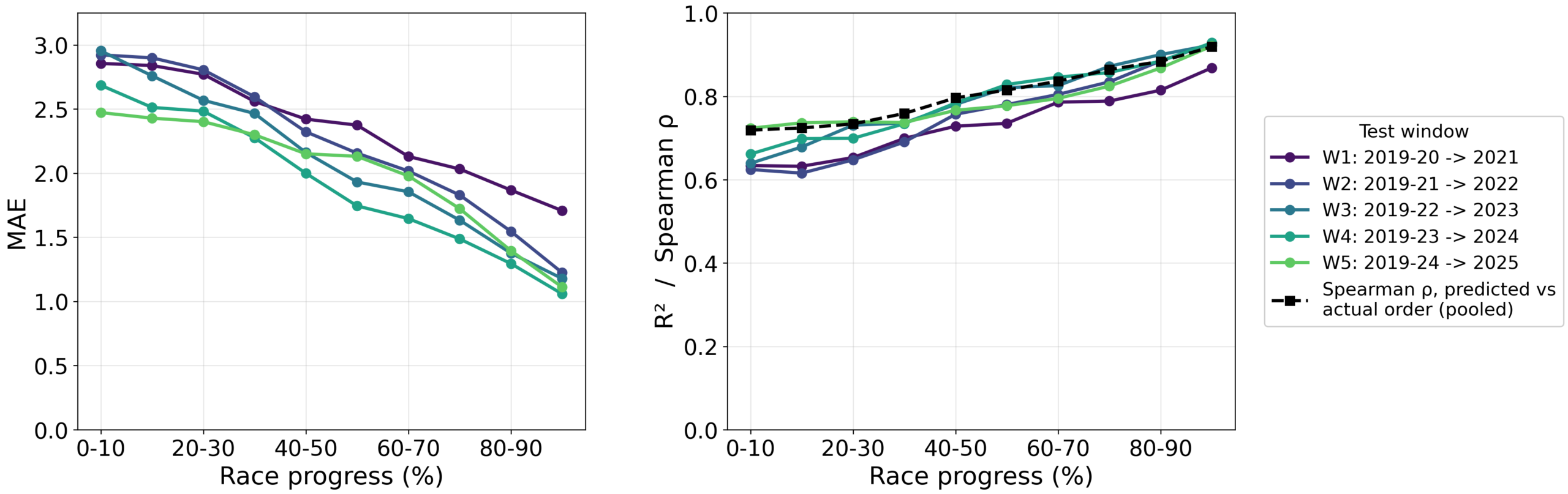
Figure 1 shows how XGBoost’s accuracy changes over the course of the race, with MAE per tenth of a race in Figure 1 (left) and R² per tenth of a race in Figure 1 (right). Each lap is assigned into a race progress bucket (0-10% through 90-100%), however, since predictions begin at the fourth lap of a driver’s race at the earliest, the first bucket spans lap 4 through the 10% mark and excludes the chaotic opening laps. The two graphs point to the same conclusion, with MAE falling steadily from roughly 2.5 – 3.0 points in the first 10% of the race to about 1.1 – 1.7 by the end of the race, and R² climbing from 0.62 – 0.73 to 0.86 – 0.93. A lap in the beginning of the race asks the model to predict an outcome that is still 90% of the race away, before tire degradation, incidents, retirements, and strategy issues have occurred. Meanwhile, a lap in the end of the race mostly asks it to recognize an outcome that is already mostly set. For that reason, the beginning of the race is the more meaningful test of the model as a predictor.

Retired drivers drop out of the race progress buckets, so the later buckets only contain the cars that are still running. Rescoring the 2025 driver-races at fixed checkpoints, with a retired driver’s last prediction carried forward, still shows the 2025 MAE falling from 2.45 at the 10% checkpoint to 1.15 at the finish, with R² rising from 0.729 to 0.898 (Supplementary Figure S3). This shows that the decline is not just a survivorship effect.

Figure 1 also breaks down the differences between each window summarized in Table 4. Window 1 predicts 2021 from only two seasons of history, and one of them is the Covid shortened 2020 season, meaning it works from both the smallest and least representative sample. Later windows improve for two reasons: Each window adds another season of race outcomes, and from Window 3 onward, the training set also includes a season under the 2022 technical regulations, so the model is trained on cars that behave like the ones that it is predicting. 

The same predictions can also be scored in more practical terms on the held-out season. At lap four, XGBoost’s MAE is 2.47 with an R² of 0.72. By lap 10 it is 2.37 with an R² of 0.75, by lap 20 it is 2.28 with an R² of 0.75, and by lap 30 it is 2.13 with an R² of 0.78 (Supplementary Figure S8). Converted back into a finishing order, the predictions match the true order at a Spearman correlation of 0.83 per lap. The capped position accuracy described in the Methodology section is exactly correct 60.2% of the time across all laps (55.0% at lap four). It is within one position 80.4% of the time and within two positions 88.7% of the time (Supplementary Figure S4). Predicted position is on average 0.86 places from the actual.

Figure 2 breaks down XGBoost’s MAE by driver (top) and by track (bottom) (Supplementary Figures S1 and S2). The largest errors belong to the championship contenders, with Verstappen at roughly 4.2, followed by Hamilton, Perez, Leclerc, and Norris at around 3.3-3.5, while the usual backmarkers sit at 0.5 or less. This is because Formula 1 awards points only to the top 10 at 25-18-15-12-10-8-6-4-2-1, so nearly all of the target’s variance is at the front of the field. A single misplaced position can be worth seven points, whereas anyone outside of the top 10 scores 0. Since each track pays out the same points, most tracks sit in a much tighter band from 1.5 to 2.4. The worst are chaotic races. The Turkish Grand Prix (~4.3) and Russian Grand Prix (~4.0) only had 1 year of data, which was a race where rain heavily influenced the outcomes, as the Discussion section will talk about more. The next group down (Australia (~3), São Paulo (~2.8), Las Vegas (~2.8), Azerbaijan (~2.8)) are known for safety cars and incident heavy races. The easiest tracks such as Monaco, Japan, Mexico City, and Styria are races where overtaking is difficult and track position usually holds once established. In both panels, bars averaged over fewer windows tend to be noisier. Rookies such as Antonelli and tracks such as Turkey and Russia that only appeared in a single window are more skewed by difficult races. The narrow track spread is consistent with the ablation study below, where circuit characteristics contribute little predictive signal.

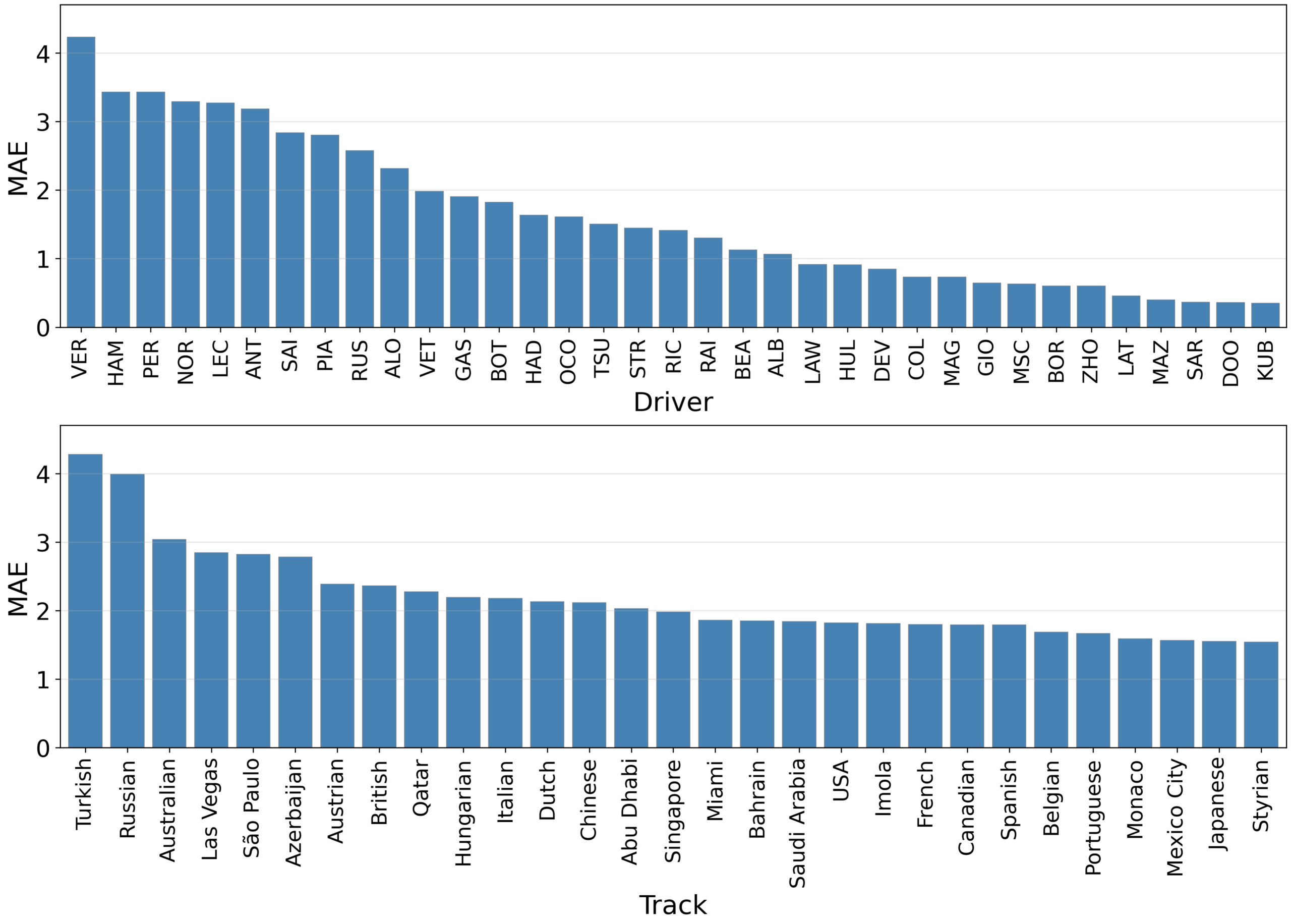
Figure 3 plots the MAE on the four selection windows at each lap number, with one line per race lag (k) depth, from 0 to 10 (the R² version is in Supplementary Figure S5). Because a model with k lags requires k prior laps, line k begins at lap k+1, and the dotted line at lap 11 marks the point from which every depth is scored on the same laps. Every line declines steadily with lap number, from roughly 2.7-3.0 points early in the race to near 1.2-1.3 by lap 70, which yet again validates the race progress pattern seen earlier. 

A depth-k model cannot be scored on laps 1 through k, which are the highest error laps in the Figure. Therefore a model which has more lags will read better due to omitting the hardest part of the race, independent of any predictive improvement. The like for like comparison is the region to the right of the lap 11 marker, where all eleven depths are evaluated on identical laps. There, all eleven depths sit inside a band of 0.12 points, and neighboring depths are often indistinguishable. For example, k = 1 and k = 2 differ by 0.004 points. Deeper models maintain a small edge, although the gain per lag falls by more than half after the third lag. Against this modest tail end benefit, each additional lag permanently removes one more early race lap from the model’s coverage, which are the laps where a lap prediction is the least redundant. We therefore set lags to k = 3, which retains predictions from the fourth lap onward while giving up little of the accuracy available to deeper configurations. This trade off between early race coverage and marginal late race accuracy is discussed further in the Limitations section.

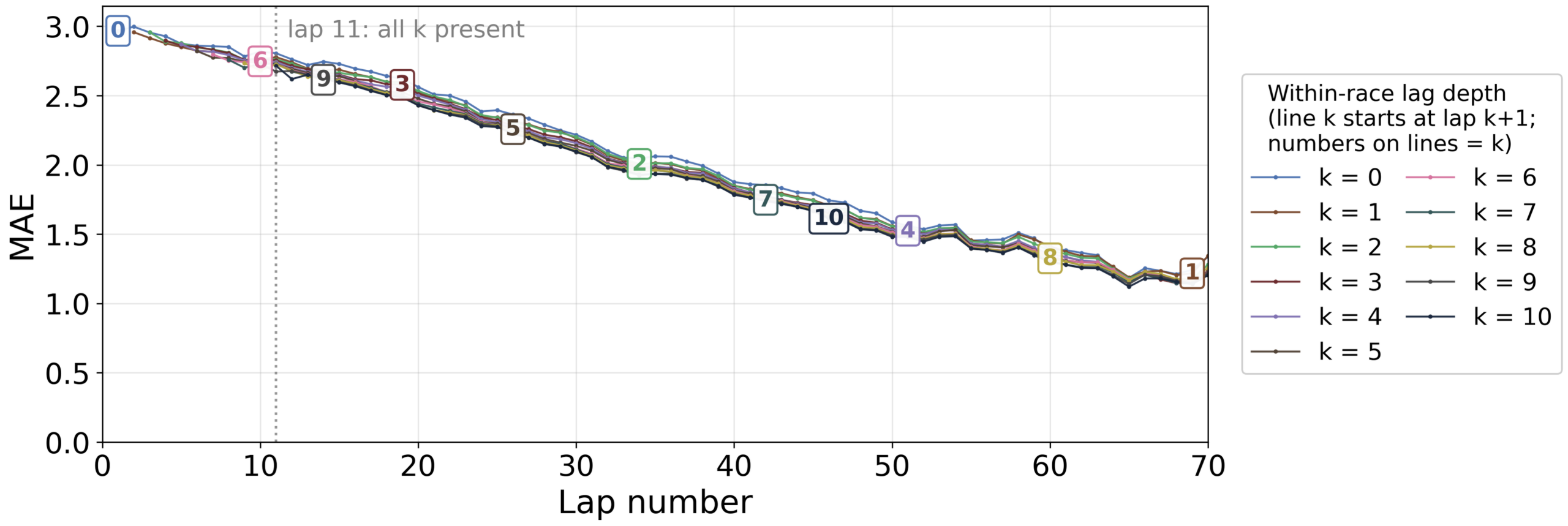
Table 6 reports the ablation on the held-out 2025 season (Supplementary Table S3). Removing the position group collapses the test R² from 0.793 to 0.418, and adds 2.2 points of MAE. It is the only category whose R² cost is distinguishable from zero. Two categories are split cases, having an MAE cost whose interval excludes zero and an R² change that does include 0. Timing and tire costs 0.12 points of MAE and weather a much smaller 0.015 points. The telemetry, circuit, and identity removals all produce intervals that span zero on both metrics. 

Category Removed	Change in R² [95% CI]	Change in MAE [95% CI]
Position	−0.3757 [−0.4371, −0.3167]	+2.1988 [+1.9341, +2.4982]
Timing & tire	−0.0068 [−0.0125, +0.0001]	+0.1238 [+0.0948, +0.1569]
Telemetry	−0.0004 [−0.0022, +0.0014]	−0.0050 [−0.0164, +0.0097]
Weather	−0.0009 [−0.0032, +0.0020]	+0.0145 [+0.0045, +0.0259]
Circuit	+0.0001 [−0.0028, +0.0028]	+0.0114 [−0.0038, +0.0283]
Identity	−0.0013 [−0.0069, +0.0037]	−0.0041 [−0.0285, +0.0192]

Discussion

The main result is that finishing points can be predicted lap by lap from public timing and telemetry data with an R² of 0.793 and a mean absolute error of 1.98 points on a held-out season that had no role in tuning or model selection (Supplementary Table S1). All four models land in a narrow band from 0.781 to 0.793 in R² and 1.98 to 2.13 in MAE, with the ordering stable. The scores are not fully stable, as a bootstrap over the 462 test driver-races gives the headline R² a 95% confidence interval of 0.729 to 0.844, so differences in the third decimal are not meaningful on their own. The ordering, however, rests on paired comparisons of the same races, and the significance tests separate every pair except LightGBM and Extra Trees on MAE. XGBoost is the best on MAE, where the clustered Diebold-Mariano test separates it from every other model in the held-out season (p < 0.0001). Second and third place depend on the metric, with LightGBM ahead of Random Forest on R² but behind it on MAE. The spread between the best and worst model (0.013 R²) is smaller than the roughly 0.06 gain from the first fold to the third and fourth as training seasons accumulate, so the choice of learner matters much less than which seasons it trains and tests on. 

The second result is that current race position and its recent history carry almost all of the predictive signal, with timing and tire at a distant second, weather third, and the rest contributing virtually nothing detectable (Table 6). However, as talked about later in the Limitations section, this comes from how we represent telemetry and not from on track behavior being uninformative. When we ran the ablation study without including last year lags, the results were essentially unchanged. The all features R² was 0.79 both ways (a difference of 0.004 R², with a 95% confidence interval spanning zero). Without the last year features, the timing and tire cost is also clear on R² (a change of -0.0087, 95% CI -0.0131 to -0.0043). We therefore consider these features as unnecessary and future work can omit them, but because they change nothing in either direction, we kept them in the reported models. 

To check the ablation picture at the level of individual features, we computed SHAP values and permutation importance for the XGBoost model on the held-out 2025 season^42,43 (Supplementary Tables S2a and S2b). The model’s built in gain importance ranks the position lags above current position. SHAP and permutation importance both place current position on top (a mean absolute SHAP of 2.23 points and a permutation R² drop of 0.31). Both methods agree with the ablation study at the category level. Position features account for 79.6% of the total SHAP attribution and 97.6% of the total permutation R² loss, with timing and tire second on SHAP at 11%, and telemetry, weather, and identity features near zero on both. Permutation assigns position a larger share than SHAP does. Every prior year feature sits at a permutation importance of approximately zero, confirming at the feature level that retaining them has no measurable effect. This is the position only baseline of the Results section seen at the feature level. 

The third result is that the difficulty is concentrated at the start of the race. Error falls continuously as the race unfolds. This early error has two main sources. Part of it is ordinary variance, as positions change most in the opening laps before the field spreads out, and there is more race left for them to change. The rest of this variance likely comes from unpredictable early race incidents, which prior work has predicted only at the whole race level, as whether a race will produce accidents at all¹², and from retirements, which Fry et al. left as future work⁵. Our largest misses fall on eventful races, which the model cannot foresee.

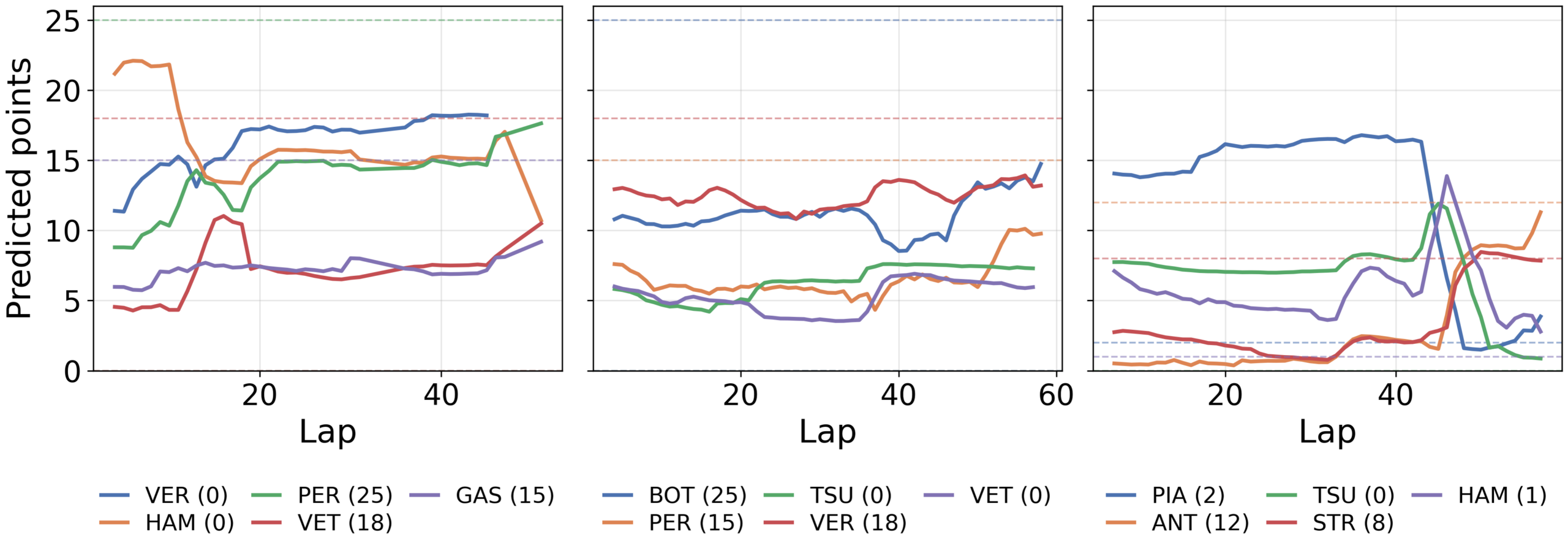
The failures are easiest seen in three distinct races. Ranked by race-level MAE, the three worst are Azerbaijan 2021 at 4.81 points (roughly twice the season average), Turkey 2021 at 4.28 points, and Australia 2025 at 3.99. Figure 4 plots the five worst predicted drivers in each one lap by lap against what they actually scored. Two of the races come down to churn, where a late reordering overturns the order the model is reading. Azerbaijan is the clearest case. Verstappen was carrying a prediction of about 18 points until his tire failed on lap 46 of 51 and brought out a red flag. In the 2 lap restart that followed, Hamilton locked up from second and scored nothing. Australia 2025 broke in the same way. A late rain shower cut Piastri from 16.5 predicted points to an actual 2, and Antonelli’s climb from 16th to 4th registered only once each place had been taken. Turkey 2021 does not fit this pattern. Of the twelve worst races it has the second highest error and the least position churn. The model held Bottas at about 11 points while he led, and he ended up scoring 25. The reason for this is likely the weather, as the race ran from start to finish on intermediate tires, with the humidity above any lap in the 2019 – 2020 training data. Every training lap above 85% humidity came from a single race, which was the wet 2019 German Grand Prix, which reshuffled its leaders. TreeSHAP attributions put the weather and tire features roughly 3 to 4 points below what the same positions drew in other 2021 races. The model was expecting a reshuffle based on the evidence it had, and none came. This does not conflict with the ablation study. Removing weather features changes accuracy by about 0.015 points of MAE across the test season (Table 6). A season average that small can still hide single races where weather matters, as Turkey 2021 did.

The comparison with the two closest studies is not a like for like benchmark. Krzysztoń and Smołka reach a macro-averaged F1 of 78% on a four class grouping of the finish from pre-race and summary features¹⁸. Fatima and Johrendt predict a driver’s rank on upcoming laps (which is a shorter horizon than our end of race target), with a test RMSE of about two positions⁸. Our task is harder than that in one sense and easier in another. It is harder because the target is a continuous points value predicted at every lap and scored forward across five seasons (four selection windows and the held-out 2025 test) spanning the 2022 regulation change, so it is exposed to the drift that a within period split hides. It is easier because the model has the live standing of the race available from the fourth lap onward.

Both claims of the Research Gap and Contribution section hold up. Lap-level points prediction holds up under forward evaluation across five seasons, the last held out from all tuning and model selection, a test of season to season generalization the earlier work did not attempt. The error analysis is specific enough to name the next features to add.

Limitations

Every in-race feature is constructed within a single driver’s race. The model never sees a gap to the car ahead or a pace comparison against the field on the current lap. The only cross-driver signal it receives is track position, which is the realized outcome of competition. Adding relative features such as gap to rival and on-lap pace-delta-to-field is the direct extension of this work.

The ablation study shows that removing all telemetry features changes our performance by under 0.003 R² and 0.02 MAE in either direction, with both intervals including zero (Table 6), indicating that telemetry adds no measurable value in the form we give it. We interpret this as a limitation of our representation rather than evidence that on track behavior is uninformative. Each lap’s telemetry is reduced to per-lap means, which discards the within lap shape where the signal would live. Speed trap and channel comparisons against nearby cars are computable from the data we already have. 

The within-race lag features require three completed laps, so the first three laps of every driver’s race (10,080 of 184,947 laps) are dropped and predictions begin at lap four or later where opening laps are incomplete. The excluded laps are the highest variance portion of the race, where start incidents reorder the field. We tuned a lag-free version of the XGBoost model to allow predictions from lap 1. In the held-out 2025 season it reached an R² of 0.69, 0.71 and 0.72 with an MAE of 2.62, 2.54 and 2.51 at laps 1, 2 and 3 (Supplementary Table S7). Across all of its laps, it reached an R² of 0.78 and an MAE of 2.07, close to the main model’s 0.79 and 1.98. The main lagged model is more accurate by 0.11 MAE at lap 12, where the two models score the same driver-races.

The choice of predicting points instead of finishing position as the target makes it such that the model cannot distinguish between positions in the bottom half of the field. Positions 11 through 20 all result in zero points, so the model receives an identical label for finishing eleventh or last. The same scoring structure concentrates error at the front of the field, where a single position can be worth seven points, so per-driver error scales with competitiveness (Figure 2).

The model predicts each driver’s laps independently, so its outputs on a given lap are not constrained to form a valid points allocation. Nothing prevents two drivers from both being predicted near 25 points on the same lap. In practice, no race in the held-out 2025 season has two drivers predicted 20 or more points at any checkpoint, and the sum of predicted points averages between 0.99 and 1.05 of the actual total (Supplementary Table S9 and Figure S7). The underlying regression treats a structured, zero inflated discrete points scale as a continuous target. On this zero-heavy target, MAE rewards predicting exactly zero, which is why the current position lookup wins on it. Tuning and selection used R² (which matches the squared error the model minimizes), so the model estimates expected points. Ranking drivers by predicted points places each one correctly inside or outside the top 10 85% of the time, and a prediction of at least half a point matches whether the driver scored 78% of the time when read as a classification on the held-out 2025 season. Two alternatives are left to future work: an ordinal model that predicts finishing position as ordered categories (as opposed to points values), and a two stage model that predicts whether a driver scores at all, and then how many points if they do. A single regression has to blend the chance of scoring and the amount of points scored into one average, while splitting them allows the model to provide an exact zero as an output for the cars that will not score and a separate estimate for the ones that will. The same independence holds across laps, as the model is never conditioned on its own earlier predictions, since the lag features carry observed quantities from previous laps, not predicted points. Each lap is scored as a fresh estimate instead of an update to a running forecast, so a driver’s predicted points can jump between consecutive laps. 

The feature set includes grid position only through the previous year’s grid at the same event, not through the race’s actual starting position. The current race position possibly absorbs most of what grid position would add, however we never tested the addition directly, and grid position is among the strongest pre-race predictors in prior works.

Finally, the dataset spans the 2022 technical regulation change, which reordered competitive performance, so patterns learned from earlier seasons may be outdated for later ones. To test this directly, we trained and tuned separate models within each era. The pre change model, trained on 2019 – 2020, tested on 2021, reached an R² of 0.734 (95% CI 0.681 to 0.781), while the post change model, trained on 2023 – 2024 and tested on 2025, reached 0.784 (95% CI 0.731 to 0.825), with overlapping intervals (Supplementary Table S8). On the shared 2025 test season, the full model trained on all seasons beat the post change model on MAE by 0.13 points (95% CI 0.07 to 0.18), while remaining statistically indistinguishable on R², so era mixing helps even with the regulation change. Both era models were tuned on a single selection window (validating on 2020 and 2024), a noisier selection than the main four window protocol. Performance under a future regulation change, such as 2026, remains uncertain.

Conclusion 

We predicted each driver’s finishing points from every lap of a race from the fourth lap onward, using data from 171 races across 2018 – 2025. We used four tree ensembles tuned under expanding-window cross-validation and tested on a single held-out season. XGBoost performed best, reaching an R² of 0.793 and a mean absolute error of 1.98 points on the held-out 2025 season. The clustered Diebold-Mariano test separates it from every other model on MAE. All four models finished within 0.013 R² of one another, a spread smaller than the ~0.06 difference between the first and later windows. The ablation shows that current race position dominates. Timing and tire, and weather information carry a small signal and everything else (telemetry in the per-lap form, circuit descriptors, driver identity, and the prior year lags) show no detectable effect. Error falls steadily as a race unfolds from roughly 2.5 MAE in the opening stages to near 1 by the end of a race. These results show that strong in-race prediction is possible from live timing and position data alone, and that the path to improvement is better inputs, such as relative features that let the model see the race as a contest and telemetry that keeps within lap structure.

Supplementary Information

References

1. Formula 1. F1 broadcast to 1.9 billion total audience in 2019. https://www.formula1.com/en/latest/article/f1-broadcast-to-1-9-billion-fans-in-2019.4IeYkWSoexxSIeJyuTrk22 2020. [↩]
2. A. Patil, N. Jain, R. Agrahari, M. Hossari, F. Orlandi, S. Dev. A data-driven analysis of Formula 1 car races outcome. in Artificial Intelligence and Cognitive Science pg. 134–146, Springer Nature Switzerland, 2023. https://doi.org/10.1007/978-3-031-26438-2_11. [↩] [↩] [↩] [↩] [↩] [↩]
3. J. Jeong, J. Y. Kim, Y. J. Ro. On the efficiency of racetrack betting market: a new test for the favourite-longshot bias. Applied Economics. Vol. 51, pg. 5817–5828, 2019, https://doi.org/10.1080/00036846.2019.1624918. [↩]
4. O. Hubáček, G. Šourek, F. Železný. Exploiting sports-betting market using machine learning. International Journal of Forecasting. Vol. 35, pg. 783–796, 2019, https://doi.org/10.1016/j.ijforecast.2019.01.001. [↩]
5. J. Fry, T. Brighton, S. Fanzon. Faster identification of faster Formula 1 drivers via time-rank duality. Economics Letters. Vol. 237, pg. 111671, 2024, https://doi.org/10.1016/j.econlet.2024.111671. [↩] [↩] [↩] [↩] [↩] [↩]
6. A. Bell, J. Smith, C. E. Sabel, K. Jones. Formula for success: multilevel modelling of Formula One driver and constructor performance, 1950–2014. Journal of Quantitative Analysis in Sports. Vol. 12, pg. 99–112, 2016, https://doi.org/10.1515/jqas-2015-0050. [↩]
7. E.-J. van Kesteren, T. Bergkamp. Bayesian analysis of Formula One race results: disentangling driver skill and constructor advantage. Journal of Quantitative Analysis in Sports. Vol. 19, pg. 273–293, 2023, https://doi.org/10.1515/jqas-2022-0021. [↩]
8. S. S. W. Fatima, J. Johrendt. Deep-Racing: an embedded deep neural network (EDNN) model to predict the winning strategy in Formula One racing. International Journal of Machine Learning. Vol. 13, pg. 97–103, 2023, https://doi.org/10.18178/ijml.2023.13.3.1135. [↩] [↩] [↩] [↩] [↩] [↩] [↩]
9. D. Thomas, J. Jiang, A. Kori, A. Russo, S. Winkler, S. Sale, J. McMillan, F. Belardinelli, A. Rago. Explainable reinforcement learning for Formula One race strategy. in Proceedings of the 40th ACM/SIGAPP Symposium on Applied Computing pg. 1090–1097, ACM, 2025. https://doi.org/10.1145/3672608.3707766. [↩] [↩] [↩] [↩] [↩]
10. A. Heilmeier, A. Thomaser, M. Graf, J. Betz. Virtual Strategy Engineer: using artificial neural networks for making race strategy decisions in circuit motorsport. Applied Sciences. Vol. 10, pg. 7805, 2020, https://doi.org/10.3390/app10217805. [↩]
11. X. Liu, A. Fotouhi. Formula-E race strategy development using artificial neural networks and Monte Carlo tree search. Neural Computing and Applications. Vol. 32, pg. 15191–15207, 2020, https://doi.org/10.1007/s00521-020-04871-1. [↩]
12. S. Dhanvanth, R. Rajesh, S. S. Samyukth, G. Jeyakumar. Machine learning-based analytical and predictive study on Formula 1 and its safety. in Proceedings of 3rd International Conference on Machine Learning, Advances in Computing, Renewable Energy and Communication pg. 257–266, Springer Nature Singapore, 2022. https://doi.org/10.1007/978-981-19-2828-4_25. [↩] [↩]
13. T. Horvat, J. Job. The use of machine learning in sport outcome prediction: a review. WIREs Data Mining and Knowledge Discovery. Vol. 10, pg. e1380, 2020, https://doi.org/10.1002/widm.1380. [↩]
14. R. P. Bunker, F. Thabtah. A machine learning framework for sport result prediction. Applied Computing and Informatics. Vol. 15, pg. 27–33, 2019, https://doi.org/10.1016/j.aci.2017.09.005. [↩]
15. E. El Haber, E. Sawaya, M. Attieh, A. Tannous, W. Ghazaly, M. Owayjan. Formula 1 race winner prediction using random forest and SHAP analysis. in 2025 International Conference on Control, Automation, and Instrumentation (IC2AI) pg. 1270–1274, IEEE, 2025. https://doi.org/10.1109/IC2AI62984.2025.10932140. [↩]
16. K. Kashyap, H. Kunder, S. Fargose, V. Nair, H. Ranka, N. Patil. Hybrid predictive modeling for Formula 1 race outcomes: integrating random forest and graph neural networks. in Proceedings of International Conference on Computing Systems and Intelligent Applications pg. 215–227, Springer Nature Singapore, 2026. https://doi.org/10.1007/978-981-96-8350-5_15. [↩]
17. E. de L. Brennand, E. Silva, G. R. Machado. Optimization of Formula 1 racing strategies: an approach based on exploratory analysis and genetic algorithms. Journal of the Brazilian Computer Society. Vol. 32, pg. 1270–1282, 2026, https://doi.org/10.5753/jbcs.2026.5833. [↩]
18. S. Krzysztoń, J. Smołka. Application of machine learning for predicting Formula 1 race results. Journal of Computer Sciences Institute. Vol. 38, pg. 81–86, 2026, https://doi.org/10.35784/jcsi.8462. [↩] [↩] [↩] [↩]
19. C. Cappello, A. Hoegh. A state-space approach to modeling tire degradation in Formula 1 racing. Journal of Sports Analytics. Vol. 12, 2026, https://doi.org/10.1177/22150218261446170. [↩]
20. T. Tulabandhula, C. Rudin. Tire changes, fresh air, and yellow flags: challenges in predictive analytics for professional racing. Big Data. Vol. 2, pg. 97–112, 2014, https://doi.org/10.1089/big.2014.0018. [↩]
21. P. Schaefer. FastF1. GitHub 2024. https://github.com/theOehrly/Fast-F1. [↩] [↩]
22. B. Peng, J. Li, S. Akkas, T. Araki, Y. Ohno, J. Qiu. Rank position forecasting in car racing. in 2021 IEEE International Parallel and Distributed Processing Symposium (IPDPS) pg. 724–733, IEEE, 2021. https://doi.org/10.1109/IPDPS49936.2021.00082. [↩]
23. A. Sasikumar, A. A. Leema, P. Balakrishnan. Data-driven pit stop decision support for Formula 1 using deep learning models. Frontiers in Artificial Intelligence. Vol. 8, pg. 1673148, 2025, https://doi.org/10.3389/frai.2025.1673148. [↩] [↩] [↩]
24. J. Todd, J. Jiang, A. Russo, S. Winkler, S. Sale, J. McMillan, A. Rago. Explainable time series prediction of tyre energy in Formula One race strategy. in Proceedings of the 40th ACM/SIGAPP Symposium on Applied Computing pg. 1082–1089, ACM, 2025. https://doi.org/10.1145/3672608.3707765. [↩]
25. D. Lock, D. Nettleton. Using random forests to estimate win probability before each play of an NFL game. Journal of Quantitative Analysis in Sports. Vol. 10, pg. 197–205, 2014, https://doi.org/10.1515/jqas-2013-0100. [↩]
26. P. Robberechts, J. Van Haaren, J. Davis. A Bayesian approach to in-game win probability in soccer. in Proceedings of the 27th ACM SIGKDD Conference on Knowledge Discovery & Data Mining pg. 3512–3521, ACM, 2021. https://doi.org/10.1145/3447548.3467194. [↩]
27. A. Groll, C. Ley, G. Schauberger, H. Van Eetvelde. A hybrid random forest to predict soccer matches in international tournaments. Journal of Quantitative Analysis in Sports. Vol. 15, pg. 271–287, 2019, https://doi.org/10.1515/jqas-2018-0060. [↩]
28. R. Baboota, H. Kaur. Predictive analysis and modelling football results using machine learning approach for English Premier League. International Journal of Forecasting. Vol. 35, pg. 741–755, 2019, https://doi.org/10.1016/j.ijforecast.2018.01.003. [↩]
29. Y. Ouyang, X. Li, W. Zhou, W. Hong, W. Zheng, F. Qi, L. Peng. Integration of machine learning XGBoost and SHAP models for NBA game outcome prediction and quantitative analysis methodology. PLOS ONE. Vol. 19, pg. e0307478, 2024, https://doi.org/10.1371/journal.pone.0307478. [↩]
30. S. A. Kovalchik. Searching for the GOAT of tennis win prediction. Journal of Quantitative Analysis in Sports. Vol. 12, pg. 127–138, 2016, https://doi.org/10.1515/jqas-2015-0059. [↩]
31. L. Kholkine, T. Servotte, A.-W. de Leeuw, T. De Schepper, P. Hellinckx, T. Verdonck, S. Latré. A learn-to-rank approach for predicting road cycling race outcomes. Frontiers in Sports and Active Living. Vol. 3, pg. 714107, 2021, https://doi.org/10.3389/fspor.2021.714107. [↩]
32. F. Pedregosa, G. Varoquaux, A. Gramfort, V. Michel, B. Thirion, O. Grisel, M. Blondel, P. Prettenhofer, R. Weiss, V. Dubourg, J. Vanderplas, A. Passos, D. Cournapeau, M. Brucher, M. Perrot, É. Duchesnay. Scikit-learn: machine learning in Python. Journal of Machine Learning Research. Vol. 12, pg. 2825–2830, 2011, https://jmlr.org/papers/v12/pedregosa11a.html. [↩]
33. L. Breiman. Random forests. Machine Learning. Vol. 45, pg. 5–32, 2001, https://doi.org/10.1023/A:1010933404324. [↩]
34. P. Geurts, D. Ernst, L. Wehenkel. Extremely randomized trees. Machine Learning. Vol. 63, pg. 3–42, 2006, https://doi.org/10.1007/s10994-006-6226-1. [↩]
35. T. Chen, C. Guestrin. XGBoost: a scalable tree boosting system. in Proceedings of the 22nd ACM SIGKDD International Conference on Knowledge Discovery and Data Mining pg. 785–794, ACM, 2016. https://doi.org/10.1145/2939672.2939785. [↩]
36. G. Ke, Q. Meng, T. Finley, T. Wang, W. Chen, W. Ma, Q. Ye, T.-Y. Liu. LightGBM: a highly efficient gradient boosting decision tree. in Advances in Neural Information Processing Systems 30 Curran Associates, 2017. https://papers.nips.cc/paper/6907-lightgbm-a-highly-efficient-gradient-boosting-decision-tree. [↩]
37. C. Spearman. The proof and measurement of association between two things. The American Journal of Psychology. Vol. 15, pg. 72–101, 1904, https://doi.org/10.2307/1412159. [↩]
38. C. Bergmeir, J. M. Benítez. On the use of cross-validation for time series predictor evaluation. Information Sciences. Vol. 191, pg. 192–213, 2012, https://doi.org/10.1016/j.ins.2011.12.028. [↩]
39. J. Demšar. Statistical comparisons of classifiers over multiple data sets. Journal of Machine Learning Research. Vol. 7, pg. 1–30, 2006, https://jmlr.org/papers/v7/demsar06a.html. [↩]
40. F. X. Diebold, R. S. Mariano. Comparing predictive accuracy. Journal of Business & Economic Statistics. Vol. 13, pg. 253–263, 1995, https://doi.org/10.1080/07350015.1995.10524599. [↩]
41. S. Holm. A simple sequentially rejective multiple test procedure. Scandinavian Journal of Statistics. Vol. 6, pg. 65–70, 1979, https://www.jstor.org/stable/4615733. [↩]
42. S. M. Lundberg, S.-I. Lee. A unified approach to interpreting model predictions. in Advances in Neural Information Processing Systems 30 Curran Associates, 2017. https://papers.nips.cc/paper/7062-a-unified-approach-to-interpreting-model-predictions. [↩]
43. A. Fisher, C. Rudin, F. Dominici. All models are wrong, but many are useful: learning a variable’s importance by studying an entire class of prediction models simultaneously. Journal of Machine Learning Research. Vol. 20, pg. 1–81, 2019, https://jmlr.org/papers/v20/18-760.html. [↩]