Deep Learning Biomedical Application: Finger Movement Recognition Through Time Series Classification of Electromyographic Signals

Abstract

Electromyographic (EMG) signal classification is vital but remains challenging for advanced prosthetics and medical diagnostics, especially when the number of movement classes increases. While the field favors convolutional neural networks (CNNs), they require more computational resources than small prosthetic devices can handle. Thus, we compared CNNs with simpler feedforward neural networks (FFNNs) to explore whether a lower-complexity model can match CNNs’ accuracy in multi-class EMG signal classification. EMG signals of 12 basic finger movements from 27 subjects were retrieved from the publicly available Ninapro database, preprocessed using Butterworth and Bandpass filters, and five standard time-domain features were extracted. We tested multiple FFNN and CNN models – each architecture evaluated across 5 runs – to compare the optimal model for 4-, 8-, and 12-class classification; mean accuracy, standard deviation, precision, recall, F1-score, error maps, and loss curves were generated for further analysis. Results showed that FFNNs consistently outperformed CNNs in mean and max accuracy for all three class counts (p < 0.001), with the gap widening as the number of classes increased: roughly 4.4% at 4-class, 6.4% at 8-class, and 7.5% at 12-class. Both models, especially CNNs, struggled with overfitting and classification of thumb exercises (movements M9-M12). Contrary to the field’s modern preference for CNNs, simpler FFNNs performed better in EMG signal classification, with their advantage growing as the number of classes increased. This suggests that FFNNs may be a more accurate and computationally efficient alternative to CNNs for resource-constrained EMG-based applications like prosthetic control.

Keywords: Electromyography (EMG), movement/gesture recognition, feedforward neural network (FFNN), convolutional neural network (CNN), deep learning, computer science, biomedical application

Introduction

Electromyogram (EMG) signals are electrical changes in the skeletal muscle captured during muscle contraction¹ by using sensors implanted in or placed on the skin². Within the biomedical field, analyzing these signals for real-time finger movement recognition and classification is foundational for detecting neuromuscular abnormalities, evaluating neurorehabilitation methods³, and developing advanced neuroprosthetic control⁴ to restore natural dexterity and autonomy for individuals with limb amputations or neuromuscular deficiencies^5,6.

Despite its clinical importance, robust automated multi-class classification of EMG signals using deep learning (DL) remains a challenge due to the “chaotic nature” of noise present among the continuously changing time-domain information of myoelectric signals^1,7. The difficulty grows especially when using public databases with a larger number of target movement classes to simulate real-world clinical signal complexities, as subtle variations often lead to large drops in classification accuracy^8,9,10.

To tackle this problem, contemporary research heavily favors the use of Convolutional Neural Networks (CNNs) and their spatial feature extraction^5,11, which yield high movement classification accuracy^12,13,14,15. Specifically, Geng developed a CNN gesture recognition model achieving 99.5% accuracy using a highly controlled, unique dataset⁸. However, other studies using the publicly available Ninapro datasets for their models noted relatively low performances; Hu’s and Wei’s models topped off at 87.0% and 82.2% accuracy, respectively^9,10. While many studies utilize CNNs and other complex architectures to achieve high accuracy, they typically require heavy computational models¹⁶, longer training times, and experience an increased risk of overfitting. These limitations trickle down to real-life concerns, such as rapid battery drain and thermal dissipation in wearable prosthetics that rely on small embedded microcontrollers to function¹⁷. This makes heavy sequential frameworks impractical for daily use.

To address this, our study compared a baseline Feedforward Neural Network (FFNN) model against a spatial CNN to evaluate whether a lower-complexity model can achieve comparable performance in multi-class EMG classification, mitigating the concerns and offering a more cost- and time-efficient alternative for clinical application. The FFNN approach maps non-linear signals globally and passes information forward through weighted processing nodes¹⁸, while the CNN approach specializes in recognizing localspatial patterns via convolutional kernels¹⁹. Because the study specifically prioritizes investigating whether minimized computational weight—i.e., basic FFNNs—can maintain competitive classification performance under realistic signal data, complex sequential architectures such as Long Short-Term Memory (LSTMs) networks or Gated Recurrent Units (GRUs) are excluded from our scope of research.

Following the general experimentation methods of previous studies conducted^20,21, we used a Ninapro dataset of EMG signals from 27 healthy subjects^22,23,24,25 to test each architecture on classifying 4, 8, and 12 distinct finger gesture movements from Exercise 1. The signals were preprocessed using two filters and extraction of five time-domain features, and the models were adjusted (i.e., number of neurons for FFNNs, and kernel size and number of feature maps for CNNs) to find the optimal architecture for classifying different numbers of gestures. Each architecture was run five times, and the mean accuracy and standard deviation (SD), as well as Precision, Recall, and F1-Score values, were recorded, along with its error map and training loss graph. Then, the mean accuracy of CNNs and FFNNs for each number of classes was compared using a t-test to yield a p-value.

However, a primary limitation of this research comes from our database, which is the publicly available Ninapro database containing pre-recorded EMG data. Consequently, the dataset lacks biological signal variability, shifting from the typical clinical target populations such as individuals with severe neuromuscular deficiencies or amputations. Furthermore, our model’s performance results are only applicable to the pre-recorded EMG signals in the Ninapro database and would perform poorly in real-life signal analysis.

Methods

Research Design

The study is an experimental, comparative performance evaluation that uses a publicly available Ninapro database to assess the accuracy of each combination of CNN or FFNN architectures and the number of signals classified, built in Google Colab using Python code.

Data Sample and Collection

The dataset was derived from Ninapro, a publicly available EMG database supporting research in movement recognition for advancements in prosthetic control. The specific dataset contains EMG signals from 27 healthy subjects (20 males, 7 females; 25 right-handed, 2 left-handed; age 28 ± 3.4 years) doing 52 different exercises, collected from 10 Otto Bock MyoBock 13E200 electrodes or sensors on the forearms^22,23,24,25.

For this experiment, we used signal data from Exercise 1 (12 basic finger gestures) repeated 10 times per subject, due to its simple, workable dataset.

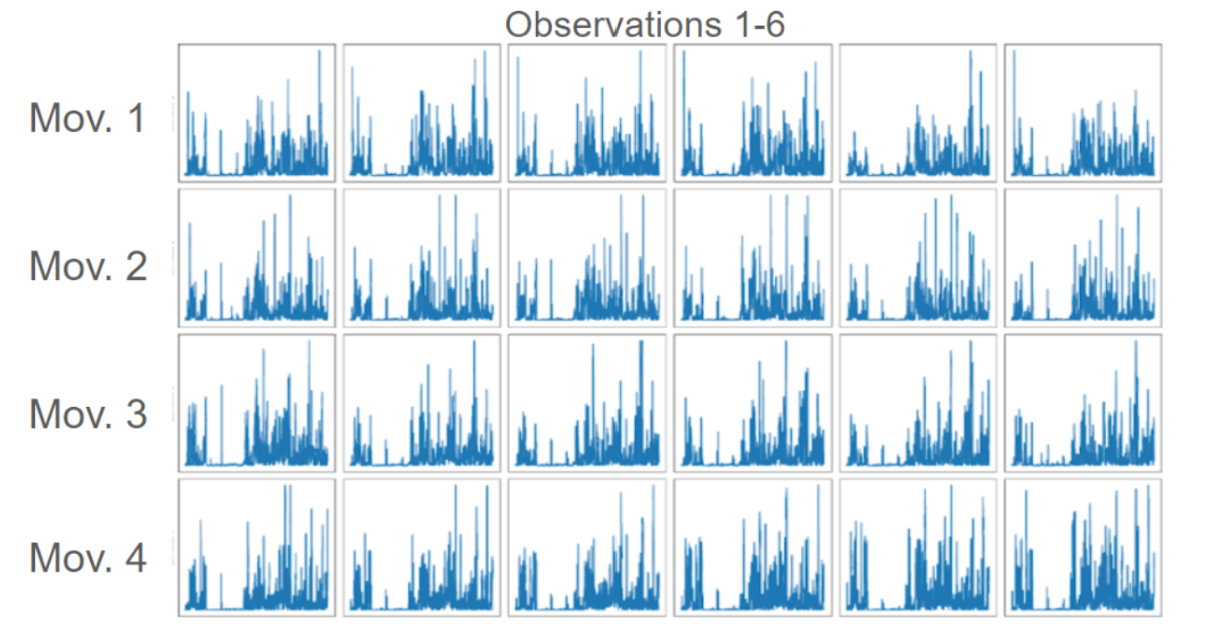
Figure 1 below shows a visual representation of the raw EMG signals from the Ninapro database we used.

Variables and Measurements

To evaluate the accuracy of different DL models, we varied the model architecture and the number of signal classes for classification, and measured the accuracy, SD, Precision, Recall, and F1-Score for each model.

Independent Variables

i. Model Architecture

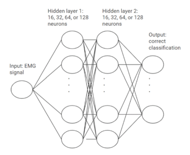
FFNN: The models transformed the input data through 2 hidden layers, each with varying numbers of neurons (16, 32, 64, 128), which processed the information to classify the signal into one of 12 gestures. The basic architecture is shown in Figure 2. We varied the number of neurons for each layer and tested all combinations.

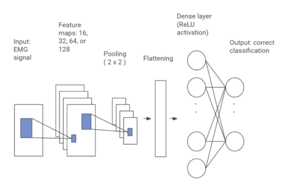
CNN: Models transformed the input data through 1 hidden layer with varying numbers of feature maps (16, 32, 64, 128) and kernel sizes (3×3, 5×5, and 7×7). Then, a 2×2 max pooling and flattening simplified the data to prepare it for input to the dense layer or fully connected layer. The basic architecture is shown in Figure 3. We modified the number of feature maps and kernel sizes and tested all combinations.

ii. Number of Signal Gestures

Each model architecture was tested for classifying different numbers of gestures from 1 to 12, 5 times per number of classes. Specifically, we tested classifications for 4 (Gesture 3, 7, 10, 12), 8 classes (Gesture 1, 3, 5, 7, 8, 10, 11, 12), and all 12 gestures. Though we initially planned to classify two gestures at a time, starting with 4 yielded unexpectedly high accuracy, prompting us to experiment with more classes.

Dependent Variables (Performance Measurements)

Classification Accuracy: We ran 5 independent iterations per model architecture to account for variability in training stability and random network weightings, and recorded the mean percent accuracy (± SD).

Predictive Diagnostics: For further analysis on class-specific classification reliability, Precision, Recall, and F1-Scores were measured. Precision records how resistant the model is to false-positive classifications for a specific class. Recall tracks the rate of false negatives or “missed” classifications per class. F1-Scores measure the harmonic mean of Precision and Recall values, serving as an overall evaluation of classification stability²⁶.

Procedure

The entire model performance evaluation was done using the Python code engineered in Google Colab, executed chronologically through the following steps:

Data Loading

The raw signal files (MATLAB format or .mat) from the Ninapro database were downloaded, unzipped, and imported into the local Google Drive with the following file naming convention: S# was used for each subject, A# was used for the acquisition number or attempt, and E# was used for the specific sets of exercises within the same acquisition. For example, S1_A1_E1 would imply that the file contains signals from Subject 1 performing movements from Exercise 1 (Gestures 0-12) during Acquisition 1.

Then, only the A1_E1 files for each subject were loaded, and the Python tool scipy.io.loadmat was used to parse the .mat files into readable Python dictionaries. From these files, the code extracted EMG signals and the categorical integer labels indicating which gesture each signal corresponds to, by accessing the ‘emg’ and ‘stimulus’ columns, respectively.

Using NumPy, the data from all 27 subjects were concatenated into a unified continuous EMG signal.

Finally, the code checked whether the total length of the continuous EMG signal matched the length of the stimulus column, ensuring that each signal reading segment synchronized with the gesture label.

Data Preprocessing: For data preprocessing, the frequency boundaries were defined as lowcut = 20.0 Hz and highcut = 450.0 Hz, and the sensor recording speed was set to fs = 1000.0 Hz.

Then, the EMG dataset was filtered using a Butterworth filter for noise reduction and a Bandpass filter for each EMG channel to normalize the signals²⁷.

Butterworth filter: By flattening the signals at a sampling rate of 0.5 fs (frequency cut to 500 Hz), this filter simplified the EMG signals for easier segmentation of essential from non-essential signals²⁸. Then, the upper and lower frequency boundaries were divided by 500 Hz to normalize the raw cutoff Hz values. These normalized frequencies were processed by the Butterworth function to generate coefficients (b and a) that act as a “fence” to block unwanted noise.

Bandpass filter: After the Butterworth filter, the Bandpass filter was used to physically block low-frequency (below 20 Hz) and high-frequency (above 450 Hz) signals from the raw continuous EMG signal, excluding unnecessary information from the signals²⁹.

Once the data were filtered using these functions, the mean signal value for each of the 10 channels was calculated and subtracted from the data, resetting the sensor baseline to zero and preventing shift of signals due to sensor or recording variability.

Finally, the continuous signal is cut into 200-ms intervals. 

Figure 4 shows a visual representation of the completely filtered EMG signal output at the end.

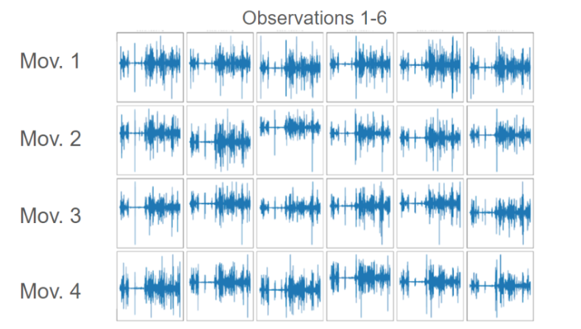
Time-Domain Feature Extraction: Next, feature extraction was done as follows: 5 features x 10 channels = 50 total features were extracted per 200-ms window.

As for the features, five important types for classifying EMG signals³⁰ were selected:

Mean absolute value (MAV): This determines the average height or amplitude of the EMG signals³¹, which helps determine the variability of the muscle stimulus and estimate the motion range²².

Root mean square (RMS): This determines the total power of the signals, which helps detect the spikes in the signals that signify the stimulus or movement of muscles³².

Variance (VAR): This determines how much the signal varies from the average value³³.

Wavelength (WL): This determines the length of each wave of signals, indicating how complex and fast the signals are waving³⁴.

Number of Zero Crossings (ZC): This determines the number of times the EMG signals have crossed the x-axis, which helps estimate the overall shape of the signals (i.e., how crowded they are)³⁵.

We chose these five features not only because they are commonly used in EMG signal analysis, but also because they are simple, lower-computational features that are efficient compared to complex ones.

Class Selection and Relabeling: After feature extraction, Class 0, or the resting (non-movement) state, was excluded from classification. The remaining Classes 1-12 were relabeled as 0-11, since deep learning frameworks expect class labels to begin at 0. Then, specific subsets of these classes were selected for each experiment to evaluate 4-class, 8-class, and 12-class classification performance, in order to observe patterns between the number of classes and model accuracy. After each class subset was selected, LabelEncoder was applied to re-index the labels contiguously, accounting for the numeric gaps from the excluded classes.

Data Split: Then, the data were split into 3 sets: 60% for training, 20% for validation, and 20% for testing. Each split was stratified to preserve the original class proportions. Furthermore, StandardScaler was fit only on the training data and was then used to scale the validation and testing data to prevent data leakage.

Model Architecture Configuration: FFNNs used 16, 32, 64, or 128 neurons in the first and second layers, and all 16 combinations of these neuron counts across the two layers were tested (an example architecture would be 16 neurons for the first layer and 128 neurons for the second layer, e.g., 16 x 128). CNNs used 3×3, 5×5, or 7×7 kernel sizes and 16, 32, 64, or 128 feature maps, and all 12 combinations of these kernel sizes and feature map counts were tested (an example architecture would be 3×3 kernel size and 128 feature maps, e.g., 3×3, 128).

This marks one full 4-class classification experiment. Each architecture was tested 5 times.

This was repeated with 4, 8, and 12 subset classes for the 4-, 8-, and 12-class classification experiments, respectively.

Training Methodology and Input: The Adam optimizer with a starting learning rate of 0.001 was used to control the size of each weight adjustment during training, minimizing loss. The sparse_categorical_crossentropy loss function was used to measure the difference between the model’s prediction and the actual class, since the class labels are expressed as integers rather than one-hot vectors (0 or 1). Batch size was set to 32 during training via model.fit(). EarlyStopping was used to prevent overfitting by stopping training when validation loss failed to improve for x epochs in a row, referred to as patience (x = 7 for FFNN and x = 10 for CNN), and restoring the model’s best-performing weights once triggered. Table 1 below shows the specific hyperparameters used for training the models, which were kept constant throughout the experiments.

Hyperparameter	Value
Optimizer	Adam
Learning rate	0.001
Batch size	32
Max epochs	100
Early stopping monitoring	Validation loss
Early stopping patience	7 (FFNN) / 10 (CNN)
Activation function	ReLU
Loss function	Sparse categorical crossentropy
Number of runs per architecture	5

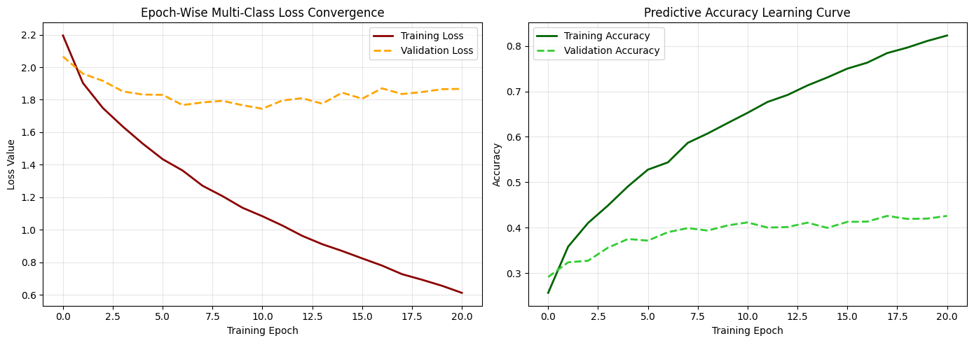
Evaluation: Test accuracy was computed for each architecture by calculating the mean and SD of the 5 runs per architecture, which is further discussed in Data Analysis. Classification_report was used to generate precision, recall, and F1-score per architecture for further analysis of the model performance. Additionally, training loss versus validation loss, and training accuracy versus validation accuracy, were plotted for each architecture to evaluate convergence. For instance, a decreasing training loss along with a rising validation loss indicates overfitting, while both losses remaining high indicate underfitting, and the flattening and converging of both losses indicate healthy training. Finally, a confusion matrix was used to generate an error map per architecture, helping visualize class-specific misclassification patterns.

Data Analysis

For each number of subset classes, the mean accuracy ± SD was calculated for FFNN and CNN to compare whether one outperformed the other. Then, an unpaired t-test was performed using all accuracies in each number of subset classes from FFNN and CNN to evaluate whether the difference in accuracy between FFNN and CNN was statistically significant – a p-value < 0.05 was considered evidence of a significant difference, with a p-value < 0.01 indicating an even stronger statistical confidence in that difference.

Ethical Considerations

Our study used a secondary, publicly available, de-identified dataset from the Ninapro database. Responsibility for obtaining informed consent or any ethical approval for the original data collection lies with the Ninapro research team, whose acquisition protocol is described in their original publications^22,23,24,25. Since this is a computational analysis on already-existing data, no new ethical concerns were introduced.

Results

After performing all classifications with variants of FFNN and CNN architectures, we found that FFNN accuracy (both mean and max) surpassed CNN accuracy in all 4-, 8-, and 12-class classifications, with p-values < 0.01 (strong significance). In addition, the classification accuracy difference between the two models increased as the number of classes to classify increased. Table 2 below summarizes and compares the accuracy of FFNN and CNN architectures.

# of classes	Best FFNN Architecture	Best FFNN Accuracy (%)	FFNN Mean (%)	Best CNN Architecture	Best CNN Accuracy (%)	CNN Mean (%)	p-value	Significant?
4	128×64	70.82	67.96	5×5, 128	67.10	63.57	0.000402	Yes
8	128×128	58.01	51.99	7×7, 128	49.40	45.62	0.000021	Yes
12	128×128	51.46	44.74	7×7, 128	41.47	37.23	0.000004	Yes

Tables 3-8 present the specific mean accuracy, STD, precision, recall, and F1-scores per architecture per 4-, 8-, and 12-class classifications, with the best-performing architecture highlighted in orange per table. As shown in Tables 3 and 4, 128×64 and 5×5, 128 were the best architectures for FFNN and CNN, respectively, in 4-class classification. From Tables 5 and 6, 128×128 and 7×7, 128 were the best architectures for FFNN and CNN, respectively, in 8-class classification; the same architectures performed best in 12-class classification, as indicated in Tables 7 and 8. Across most architectures, accuracy generally increased as the number of neurons, kernel size, or feature maps increased.

Layer 1 – # neurons	Layer 2 – # neurons	Mean Accuracy (%)	Std (%)	Macro Precision	Macro Recall	Macro F1-Score
16	16	63.73	1.5	0.62	0.62	0.61
16	32	64.73	1.31	0.64	0.64	0.64
16	64	64.66	1.47	0.66	0.66	0.66
16	128	66.13	0.91	0.66	0.66	0.66
32	16	67.99	1.31	0.67	0.67	0.67
32	32	67.49	0.82	0.68	0.68	0.68
32	64	67.99	1.91	0.7	0.7	0.69
32	128	68.75	1.58	0.71	0.7	0.7
64	16	67.13	1.32	0.69	0.69	0.68
64	32	70.14	0.9	0.7	0.7	0.7
64	64	70.04	1.45	0.69	0.68	0.69
64	128	69.82	0.83	0.69	0.69	0.69
128	16	68.6	1.23	0.67	0.67	0.67
128	32	69	1.07	0.69	0.7	0.69
128	64	70.82	2.05	0.68	0.68	0.68
128	128	70.32	1.35	0.7	0.7	0.7

Kernel Size	# Feature Maps	Mean Accuracy (%)	Std (%)	Macro Precision	Macro Recall	Macro F1-Score
3×3	16	56.85	0.82	0.57	0.56	0.57
3×3	32	61.94	0.7	0.61	0.61	0.61
3×3	64	64.87	1.29	0.67	0.67	0.66
3×3	128	65.95	1.29	0.65	0.65	0.64
5×5	16	60.5	1.83	0.58	0.59	0.58
5×5	32	62.9	1.72	0.65	0.64	0.64
5×5	64	65.13	0.66	0.65	0.65	0.65
5×5	128	67.1	1.21	0.65	0.65	0.65
7×7	16	61.22	1.89	0.58	0.58	0.58
7×7	32	64.12	1.1	0.64	0.64	0.64
7×7	64	65.63	1.14	0.64	0.64	0.64
7×7	128	66.67	1.26	0.66	0.65	0.65

Layer 1 – # neurons	Layer 2 – # neurons	Mean Accuracy (%)	Std (%)	Macro Precision	Macro Recall	Macro F1-Score
16	16	45.22	1.38	0.48	0.48	0.47
16	32	47.23	1.81	0.48	0.48	0.47
16	64	47.98	0.99	0.48	0.48	0.48
16	128	50.49	1.08	0.51	0.51	0.5
32	16	48.22	0.71	0.47	0.47	0.47
32	32	50.49	1.21	0.49	0.49	0.49
32	64	52.14	1.18	0.52	0.52	0.51
32	128	53.29	0.8	0.54	0.54	0.54
64	16	50.64	0.75	0.52	0.52	0.51
64	32	51.89	1.74	0.54	0.54	0.54
64	64	53.9	0.94	0.55	0.55	0.54
64	128	55.55	1.04	0.54	0.54	0.54
128	16	53.97	1.12	0.55	0.55	0.55
128	32	55.62	1.45	0.57	0.56	0.56
128	64	57.18	0.68	0.57	0.57	0.57
128	128	58.01	0.9	0.6	0.59	0.59

Kernel Size	# Feature Maps	Mean Accuracy (%)	Std (%)	Macro Precision	Macro Recall	Macro F1-Score
3×3	16	40.7	0.84	0.39	0.4	0.39
3×3	32	44.11	1.07	0.42	0.42	0.42
3×3	64	45.78	0.48	0.46	0.46	0.46
3×3	128	47.84	0.8	0.47	0.47	0.47
5×5	16	41.58	1.08	0.42	0.42	0.42
5×5	32	44.57	0.84	0.44	0.44	0.43
5×5	64	48	1.08	0.48	0.48	0.47
5×5	128	48.86	0.99	0.49	0.48	0.47
7×7	16	43.3	0.64	0.43	0.43	0.43
7×7	32	46.15	1.28	0.47	0.48	0.47
7×7	64	47.19	0.82	0.48	0.48	0.48
7×7	128	49.4	1.2	0.49	0.49	0.48

Layer 1 – # neurons	Layer 2 – # neurons	Mean Accuracy (%)	Std (%)	Macro Precision	Macro Recall	Macro F1-Score
16	16	37.48	0.98	0.35	0.35	0.35
16	32	39.96	0.93	0.42	0.41	0.41
16	64	41.75	1.57	0.4	0.39	0.39
16	128	44.01	1.12	0.44	0.44	0.44
32	16	40.71	1.22	0.42	0.42	0.41
32	32	42.28	0.73	0.42	0.42	0.42
32	64	43.76	1.77	0.44	0.43	0.43
32	128	46.1	1.44	0.48	0.48	0.47
64	16	42.95	1.88	0.44	0.45	0.44
64	32	43.91	1.31	0.45	0.45	0.45
64	64	47.78	0.86	0.46	0.47	0.46
64	128	50.73	0.82	0.52	0.52	0.51
128	16	45.55	1.54	0.43	0.43	0.43
128	32	48.28	0.81	0.48	0.47	0.47
128	64	49.07	0.38	0.5	0.5	0.5
128	128	51.46	1.14	0.52	0.52	0.52

Kernel Size	# Feature Maps	Mean Accuracy (%)	Std (%)	Macro Precision	Macro Recall	Macro F1-Score
3×3	16	32.85	1.16	0.32	0.32	0.31
3×3	32	35.14	0.52	0.36	0.35	0.34
3×3	64	36.79	1.11	0.36	0.37	0.36
3×3	128	39.8	0.76	0.4	0.39	0.39
5×5	16	33.23	1.07	0.33	0.32	0.32
5×5	32	36.28	0.94	0.37	0.37	0.37
5×5	64	38.66	0.83	0.39	0.39	0.39
5×5	128	40.06	0.84	0.43	0.41	0.41
7×7	16	34.82	0.45	0.34	0.35	0.34
7×7	32	38.21	0.86	0.38	0.38	0.38
7×7	64	39.49	0.77	0.4	0.4	0.39
7×7	128	41.47	0.35	0.42	0.42	0.42

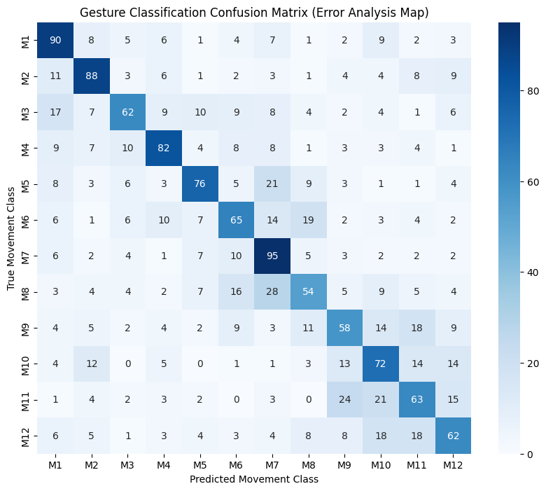
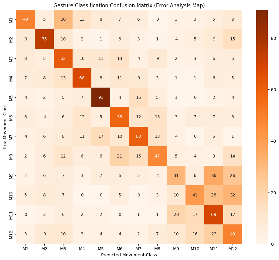
Furthermore, confusion matrices were generated for each architecture to analyze precision and recall for each class. For convenience, we have included the confusion matrices for the best-performing FFNN and CNN architectures for 12-class classification, as they contain the most information for analysis. Figures 5 and 6 show that both models often misclassified movements M9-M12 as one another, becoming a “confusion cluster” as indicated by the relatively shaded bottom right corner in the confusion matrices.

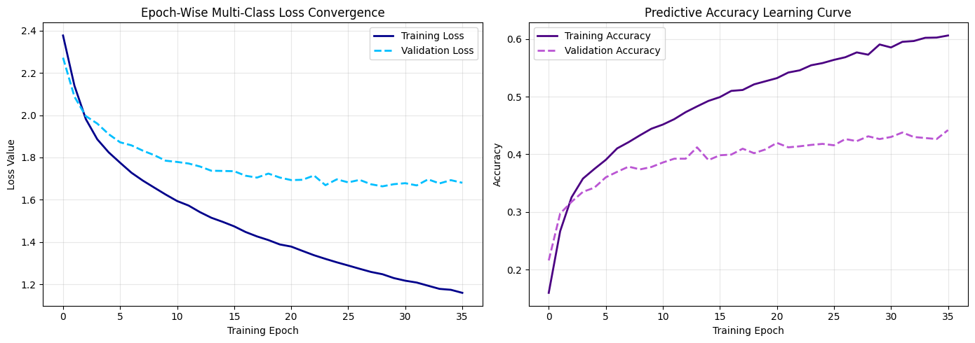
In addition to the confusion matrices, loss/accuracy curves were graphed for the best-performing FFNN and CNN architectures for 12-class classification. From Figure 7, it can be seen that both losses decreased and reached a plateau, while the accuracy of the FFNN model increased and also reached a plateau. For the CNN model, Figure 8 shows that the training loss decreased while the validation loss remained relatively unchanged, and the training accuracy increased while the validation accuracy remained relatively unchanged as well.

Discussion

Restatement of Key Findings

For 4-, 8-, and 12-class classifications, FFNN outperformed CNN in both mean and max accuracy, with the gap widening for mean accuracy as the number of classes increased: roughly 4.4% at 4-class, around 6.4% at 8-class, and over 7.5% at 12-class.

Moreover, Figures 5 and 6 revealed that both models struggled to classify movements 9-12, forming a confusion cluster in which signals were consistently misclassified as one another rather than with any other movement class. One possible explanation is that movements M9-M12 in Exercise A are thumb adduction, abduction, flexion, and extension – all thumb movement signals²³. Thumbs have their own intrinsic muscles that rely on movement, while other fingers move via the flexions and extensions of the forearm muscles³⁶. Given that the sensors used to collect these signals were placed on the subjects’ forearms, they may have struggled to capture signals from the thumb muscles, making thumb movement more difficult for both models than for other finger movements. Notably, CNN struggled with this confusion more than FFNN; for example, CNN’s precision for M9 was 0.33 compared to FFNN’s 0.46. Similarly, CNN’s precision for M12 was 0.27 compared to FFNN’s 0.47. This suggests that while FFNN performed better overall, it especially outperformed CNNs in classifying the hardest-to-distinguish thumb movements.

Furthermore, Figures 7 and 8 show that for both FFNN and CNN models, training loss steadily decreased, while validation loss initially decreased slightly before quickly plateauing. As for the learning curves for both FFNN and CNN models, training accuracy steadily increased while validation accuracy quickly plateaued. This divergence between training and validation performance indicates that both models overfitted the training data and could not perform as well during validation. Specifically, CNN suffers more overfitting since its model’s gap between training and validation loss is around 1.2, which is greater than the 0.5 gap of the FFNN model. This greater overfitting may help explain the relatively low overall accuracy of CNNs when compared to FFNNs.

Implications and Significance

While we did not specifically measure training time or parameter count, we can generalize that FFNNs have simpler architectures and thus operate quickly with fewer parameters and resources, compared to CNNs. And since all class-number classifications showed that FFNN models outperformed CNN models in EMG signal classification, it indicates that CNNs may not be practical for wearable prosthetics due to their complex architecture that leads to battery drain and overheating of devices, in addition to their relatively low accuracy in this study. On the other hand, FFNNs show great potential for prosthetic control due to their relatively stable classification performance despite their simple architecture – despite there being limitations in being able to perform well only with pre-recorded data of healthy subjects, and their performance on assessing real-time messy data remains unknown, which will be explained in detail in the Limitations section. This goes against the field’s general preference for CNNs, presenting future research in exploring FFNNs further.

Moreover, the research revealed that both models struggled with thumb movements (M9-12), possibly due to the sensor placements on the forearms, indicating that incorporating additional sensors near the thumb might be a reasonable improvement for future EMG signal data collection.

Connection to Objectives

Our hypothesis was to compare FFNN and CNN models as “simple vs complex architectures” to explore whether a simpler model could match a more complex model’s EMG signal classification accuracy. To our surprise, the FFNN model not only matched but even surpassed the accuracy of CNNs across all class counts, with the difference growing as the number of classification classes increased. This is an interesting result that challenges the field’s default preference for using architecturally complex models like CNNs for yielding high EMG classification accuracy.

Recommendations

To establish a more optimal classification model in the future, we have determined several areas for improvement or further research.

Comparisons against other architectures

Since we only compared FFNNs and CNNs, there are still other architectures worth comparing against, such as LSTM, GRUs, etc., as noted in our Introduction. Future research comparing FFNNs to such models to see whether FFNNs’ accuracies still match the more complex models would be a meaningful study in terms of measuring how much potential FFNNs have, if at all, for prosthetic control implementation.

Underperformance of CNNs

Another valuable study would be figuring out what exactly affected the decrease in CNN accuracy as the number of classification classes increased. Although we indicated that CNNs showed signs of more overfitting as well as struggles with thumb exercise classification compared to FFNNs, the exact causes remain unknown. It could be that CNNs’ spatial pattern extraction isn’t well suited for classifying filtered, pre-recorded EMG signals and may perhaps perform better with raw, image-like data, which is yet to be researched.

Use of other datasets

Since this experiment was conducted using an already retrieved dataset from Ninapro, our results cannot be generalized for all EMG signal analysis, as most real-life data will be collected and analyzed in real time. Moreover, the dataset we used was only one small dataset from Ninapro, which could not represent the high variability of real-life EMG signals since physiological signals can vary significantly depending on the subject, method of signal retrieval, and so on. Further research using multiple datasets from Ninapro or other publicly available EMG signal records must be conducted to explore a more accurate test accuracy of both architectures as well as to reevaluate the potential of FFNNs in EMG signal classification.

Feature extraction

In our experiments, we only extracted the five commonly used features – MAV, RMS, VAR, WL and ZC – from the EMG signals before inputting them into our models. Though it helped yield relatively good results, there may exist other features that can improve the test accuracy of these models even in more complex classifications. By finding such features or combinations of features from the seven important features presented by Python Package Index (PyPI)²⁷, it can help yield the most accurate classification and optimize the deep learning architectures even further, as well as overturn our results of FFNNs outperforming CNNs.

Combinations of movement classes

For this research, we randomly chose which 4 or 8 classes to use for the 4-class and 8-class classifications, which could have skewed our results since each class has distinct shapes that could sway the performance of FFNNs and CNNs – for example, certain classes may have been easier to classify with FFNNs, which may have resulted in overall higher accuracy for FFNN models. For future research, classifying only two or three classes at a time or trying different combinations of classes to classify may help yield more concrete results on FFNN and CNN performance.

Limitations

Use of Ninapro Database: As briefly mentioned in the Recommendations section, this study used the publicly available data from the Ninapro database with only signals from healthy patients, meaning that the results aren’t generalizable to classifying signals of those with neuromuscular disorders, amputations, or other conditions who are more likely to use prosthetic devices. Furthermore, the study was conducted only by classifying pre-recorded signals, and whether the performance will be maintained for real-time classification is yet to be studied.

Overfitting: Both models showed overfitting in Figures 7 and 8, with CNNs suffering more severely than FFNNs, despite the 3-way stratified train-validation-test split of the dataset with early stopping. More adjustments to both models may help mitigate overfitting and further improve accuracy for all numbers of classes.

Conclusion

In this paper, we explored different architectures of FFNNs and CNNs to determine whether the former, simpler model can match the latter, more complex model’s performance for classification of publicly available EMG signals. Our results – organized in Tables 2 through 8 – showed that FFNNs outperformed CNNs in all 4-, 8-, and 12-class classifications, with the accuracy gap growing as the number of classes increased. Our confusion maps and loss curves from Figures 5 through 8 further highlight that CNNs struggled more with thumb exercise signals and suffered more overfitting than FFNNs. This indicates FFNNs’ potential for prosthetic device optimization, serving as a potentially lower-computational-cost alternative model to CNNs. Thus, further exploration of FFNN models for EMG classification, especially for resource-constrained clinical or prosthetic applications, should be done, contrary to the field’s current preference for CNN-based model developments. Overall, the field of EMG signal classification shows great potential in the application of deep learning. Not restricted to automated physiological signal analysis, we hope research combining computer science and biomedicine continues to bloom and aid research or services in the medical field.

Acknowledgements

I would like to thank Professor Erik Sakk for his mentorship. His constructive feedback and guidance in the experimentation process have been a great help in organizing this paper.

References

1. B. Rim, N.-J. Sung, S. Min, M. Hong. Deep learning in physiological signal data: a survey. Sensors. Vol. 20, pg. 969, 2020, https://doi.org/10.3390/s20040969. [↩] [↩]
2. M.B.I. Raez, M.S. Hussain, F. Mohd-Yasin. Techniques of EMG signal analysis: detection, processing, classification and applications. Biological Procedures Online. Vol. 8, pg. 11-35, 2006, https://doi.org/10.1251/bpo115. [↩]
3. O. Faust, M.G. Bairy. Nonlinear analysis of physiological signals: a review. Journal of Mechanics in Medicine and Biology. Vol. 12, 2012, https://doi.org/10.1142/S0219519412400155. [↩]
4. O. Faust, Y. Hagiwara, T. J. Hong, O. S. Lih, U. R. Acharya. Deep learning for healthcare applications based on physiological signals: a review. Computer Methods and Programs in Biomedicine. Vol. 161, pg. 1–13, 2018, https://doi.org/10.1016/j.cmpb.2018.04.005. [↩]
5. X. Zhai, B. Jelfs, R. H. M. Chan, C. Tin. Self-recalibrating surface EMG pattern recognition for neuroprosthesis control based on convolutional neural network. Frontiers in Neuroscience. Vol. 11, 2017, https://doi.org/10.3389/fnins.2017.00379. [↩] [↩]
6. K. H. Park, S. W. Lee. Movement intention decoding based on deep learning for multiuser myoelectric interfaces. 2016 4th International Winter Conference on Brain-Computer Interface (BCI). pg. 1–2, 2016, https://doi.org/10.1109/IWW-BCI.2016.7457459. [↩]
7. N. Ganapathy, R. Swaminathan, T. M. Deserno. Deep learning on 1-D biosignals: a taxonomy-based survey. Thieme E-Journals—Yearbook of Medical Informatics. Vol. 27, pg. 98-109, 2018, https://doi.org/10.1055/s-0038-1667083. [↩]
8. W. Geng, Y. Du, W. Jin, W. Wei, Y. Hu, J. Li. Gesture recognition by instantaneous surface EMG images. Scientific Reports. Vol. 6, 2016, https://doi.org/10.1038/srep36571. [↩] [↩]
9. Y. Hu, Y. Wong, W. Wei, Y. Du, M. Kankanhalli, W. Geng. A novel attention-based hybrid CNN-RNN architecture for sEMG-based gesture recognition. PLOS ONE. Vol. 13, 2018, https://doi.org/10.1371/journal.pone.0206049. [↩] [↩]
10. W. Wei, Q. Dai, Y. Wong, Y. Hu, M. Kankanhalli, W. Geng. Surface-electromyography-based gesture recognition by multi-view deep learning. IEEE Transactions on Biomedical Engineering. Vol. 66, pg. 2964–2973, 2019, https://doi.org/10.1109/TBME.2019.2899222. [↩] [↩]
11. P. Xie, M. Xu, T. Shen, J. Chen, G. Jiang, J. Xiao, X. Chen. A channel-fused gated temporal convolutional network for EMG-based gesture recognition. Biomedical Signal Processing and Control. Vol. 95, 2024, https://doi.org/10.1016/j.bspc.2024.106408. [↩]
12. M. Atzori, M. Cognolato, H. Müller. Deep learning with convolutional neural networks applied to electromyography data: a resource for the classification of movements for prosthetic hands. Frontiers in Neurorobotics. Vol. 10, 2016, https://doi.org/10.3389/fnbot.2016.00009. [↩]
13. U. Côté-Allard, C. L. Fall, A. Drouin, A. Campeau-Lecours, C. Gosselin, K. Glette. Deep learning for electromyographic hand gesture signal classification using transfer learning. IEEE Transactions on Neural Systems and Rehabilitation Engineering. Vol. 27, pg. 760–771, 2019, https://doi.org/10.1109/TNSRE.2019.2896269. [↩]
14. W. Wang, B. Chen, P. Xia, J. Hu, Y. Peng. Sensor fusion for myoelectric control based on deep learning with recurrent convolutional neural networks. Artificial Organs. Vol. 42, pg. E272–E282, 2018, https://doi.org/10.1111/aor.13153. [↩]
15. M. Z. ur Rehman, A. Waris, S. O. Gilani, M. Jochumsen, I. K. Ziazi, M. Jamil, D. Farina, E. N. Kamavuako. Multiday EMG-based classification of hand motions with deep learning techniques. Sensors. Vol. 18, 2018, https://www.mdpi.com/1424-8220/18/8/2497. [↩]
16. N. Nguyen. Portable and Lightweight Signal Processing Approach for sEMG-Based Human–Machine Interaction in Robotic Hands. International Journal of Advanced Computer Science and Applications. Vol. 16, 2025, https://doi.org/10.14569/IJACSA.2025.0160476 [↩]
17. M. Zanghieri, S. Benatti, A. Burrello, V. Kartsch, F. Conti, L. Benini. Robust Real-Time Embedded EMG Recognition Framework Using Temporal Convolutional Networks on a Multicore IoT Processor. IEEE Transactions on Biomedical Circuits and Systems. Vol. 14, pg. 244-256, 2019, https://doi.org/10.1109/tbcas.2019.2959160. [↩]
18. W. Batayneh, E. Abdulhay, M. Alothman. Comparing the efficiency of artificial neural networks in sEMG-based simultaneous and continuous estimation of hand kinematics. Digital Communications and Networks. Vol. 8, pg. 162-173, 2022, https://doi.org/10.1016/j.dcan.2021.08.002. [↩]
19. K. Zhang, Y. Liu, M. Ferre, F. J. Badesa. EMamba: A Mamba-based framework for EMG gesture recognition via discriminative heatmap representations. Biomedical Signal Processing and Control. Vol. 121, 2026, https://doi.org/10.1016/j.bspc.2026.110296. [↩]
20. A. D. C. Chan, G. Green. Myoelectric control development toolbox. Conference of the Canadian Medical & Biological Engineering Society. 2007, https://www.researchgate.net/publication/233728145_Myoelectric_Control_Development_Toolbox. [↩]
21. M. Atzori, H. Müller. PaWFE: fast signal feature extraction using parallel time windows. Frontiers in Neurorobotics. Vol. 13, 2019, https://doi.org/10.3389/fnbot.2019.00074. [↩]
22. M. Atzori, A. Gijsberts, I. Kuzborskij, S. Elsig, A. M. Hager, O. Deriaz. Characterization of a benchmark database for myoelectric movement classification. IEEE Transactions on Neural Systems and Rehabilitation Engineering. Vol. 23, pg. 73–83, 2015, https://doi.org/10.1109/TNSRE.2014.2328495. [↩] [↩] [↩] [↩]
23. M. Atzori, A. Gijsberts, C. Castellini, B. Caputo, A. M. Hager, S. Elsig, G. Giatsidis, F. Bassetto, H. Müller. Electromyography data for non-invasive naturally-controlled robotic hand prostheses. Scientific Data. Vol. 1, 2014, https://doi.org/10.1038/sdata.2014.53. [↩] [↩] [↩] [↩]
24. M. Atzori, A. Gijsberts, S. Heynen, A. M. Hager, O. Deriaz, P. V. der Smagt, C. Castellini, B. Caputo, H. Müller. Proceedings of the IEEE Conference on Biomedical Robotics and Biomechatronics. 2012,https://publications.hevs.ch/index.php/publications/show/1172. [↩] [↩] [↩]
25. V. H. Cene, M. Tosin, J. Machado, A. Balbinot. Open database for accurate upper-limb intent detection using electromyography and reliable extreme learning machines. Sensors. Vol. 19, 2019, https://doi.org/10.3390/s19081864. [↩] [↩] [↩]
26. “FI-Score in Machine Learning.” GeeksforGeeks. https://www.geeksforgeeks.org/machine-learning/f1-score-in-machine-learning/. [↩]
27. “nina-funcs 1.0.2.” Python Package Index (PyPI). 2021, https://pypi.org/project/nina-funcs/. [↩]
28. “Butterworth Filter VI.” LabVIEW Programming Reference Manual, NI. https://www.ni.com/docs/en-US/bundle/labview-api-ref/page/vi-lib/analysis/3filter-llb/butterworth-filter-vi.html?srsltid=AfmBOoqfmP_0t6KOBl524PMpdNBmUGLtHXPg46XDlOyxG8n1kTLjI8oS. [↩]
29. “Band-pass Filters.” All About Circuits. https://www.allaboutcircuits.com/textbook/alternating-current/chpt-8/band-pass-filters/. [↩]
30. “PaWFE—Parallel-Window-Feature-Extraction.” GitHub. 2019, https://github.com/manfredoatzori/PaWFE—Parallel-Window-Feature-Extraction. [↩]
31. I. M. Khairuddin, S. N. Sidek, A. P.P. A. Majeed, M. A. M. Razman, A. A. Puzi, H. Md Yusof. The classification of movement intention through machine learning models: The identification of significant time-domain EMG features. PeerJ Computer Science. Vol. 7, pg. e379, 2021, https://doi.org/10.7717/peerj-cs.379. [↩]
32. S. Rahmatalla. Prehospital Transport and Whole-Body Vibration. 2022, https://www.sciencedirect.com/book/monograph/9780323901031/prehospital-transport-and-whole-body-vibration. [↩]
33. W. L. Thompson, G. C. White, C. Gowan. Monitoring Vertebrate Populations. 1998, https://www.sciencedirect.com/science/chapter/monograph/abs/pii/B978012688960450006X. [↩]
34. E. M.A. Hussein. Radiation Mechanics. 2007, https://www.sciencedirect.com/book/monograph/9780080450537/radiation-mechanics. [↩]
35. A. A. Torres-García,O. Mendoza-Montoya, M. Molinas, J. M. Antelis, L. A. Moctezuma, T. Hernández-Del-Toro. Biosignal Processing and Classification Using Computational Learning and Intelligence. 2022, https://www.sciencedirect.com/science/chapter/edited-volume/abs/pii/B9780128201251000142. [↩]
36. “Muscles | Hand & Upper Extremity Anatomy.” ASSH. https://www.assh.org/handcare/anatomy/muscles. [↩]