Object-Aware Image Reconstruction: Comparative Strategies for Selective Enhancement in Latent Diffusion Models

Oliver Tong

NHSJS

Object-Aware Image Reconstruction: Comparative Strategies for Selective Enhancement in Latent Diffusion Models

By

Oliver Tong

-

October 17, 2026

0

82

Read the full article as a PDF Download

Abstract

We propose a method to use Latent Diffusion Models (LDMs) for selective, object-aware image reconstruction. This method combines VAE encoding and decoding with Faster R-CNN automatic object detection and SAM segmentation. We compare four reconstruction strategies: Decoded Object Deconstruction with Fade Mask Blending (DOD-FADE) and Decoded Object Deconstruction with Segment Anything Model (DOD-SAM) operate in pixel space, while Latent Object Layering with Fade Mask Blending (LOL-FADE) and Latent Object Layering with Segment Anything Model (LOL-SAM) operate in latent space. The methods differ in both reconstruction domain (pixel versus latent space) and masking strategy (heuristic versus segmentation-guided). We evaluate them on a benchmark of 11 images covering four object categories using Fréchet Inception Distance (FID), Learned Perceptual Image Patch Similarity (LPIPS), boundary error, and a composite quality metric designed to capture edge integration, background coherence, and object preservation. FID and LPIPS favor the pixel-space methods in our benchmark, whereas boundary error favors the latent-space methods. LOL-SAM has the lowest boundary error (17.53, compared with 64.45 for DOD-SAM) and the highest composite score on 9 of the 11 images. Its mean score is 0.6546, followed by LOL-FADE (0.6006), DOD-SAM (0.5330), and DOD-FADE (0.5212). The different rankings show that the choice of metric affects how the reconstruction methods are judged, particularly when boundary integration and object preservation are more important than pixel-level similarity. We also tested mask-alpha values outside the conventional [0, 1] range. These produced localized stylization and tonal compression effects, suggesting that the framework may also be useful for controlled stylization.

Keywords: Latent Diffusion Models, Object-Aware Image Reconstruction, Image Compositing, Segment Anything Model (Sam), Variational Autoencoder, Latent-Space Blending, Perceptual Quality Metrics, Artistic Stylization

Introduction

Problem Motivation and Background

Latent Diffusion Models (LDMs), such as Stable Diffusion¹, are effective for global image synthesis, but controlling individual image regions while preserving the surrounding content remains difficult. Changing a single object while keeping its appearance, boundaries, and surrounding scene intact is particularly challenging with standard image-generation methods. We therefore focus on object-aware reconstruction, which allows selected objects to be isolated while retaining control over the rest of the image.

Formal Problem Definition

The object-aware image reconstruction problem is defined as follows: Given an input image I and a detected object region R, we isolate the foreground object and selectively process the background to reconstruct a composite image I’ with three goals:

Foreground Preservation: The object retains its original details with minimal distortion.
Background Coherence: The reconstructed background remains visually coherent and free of noticeable artifacts.
Boundary Integration: The transition between the foreground and the reconstructed background is smooth, with minimal visible compositing artifacts.

We try to maximize per-image composite quality Q_img(I’) = w_E . E + w_B . B + w₀ . O, where E, B, and O are edge transition quality, background smoothness, and object preservation, respectively. These terms are weighted by w_E = 0.45, w_B= 0.35, w₀ = 0.20 to reflect their relative visual importance.

Research Questions and Hypotheses

We study three research questions:

RQ1 (Pixel vs. Latent Domain): Do latent space methods (LOL methods) improve boundary integration and background coherence compared to pixel-space methods (DOD methods), and at what cost does this come?
H1: Latent-space methods will provide better boundary integration and background coherence than pixel-space methods, potentially at the cost of local detail preservation.
RQ2 (Heuristic vs. Segmentation-Guided Masking): Do SAM-guided segmentation masks outperform heuristic fade masks (FADE) in reducing boundary artifacts and improving boundary integration?
H2: SAM-guided masks will produce better boundary integration and fewer visible artifacts than heuristic fade masks.
RQ3 (Combined Effects): Does combining latent-space reconstruction with SAM-guided masking (LOL-SAM) improve overall composite quality compared with the other reconstruction strategies?
H3: The combination of latent-space reconstruction and SAM-guided masking will produce the highest overall composite quality.

Methodology Overview

Our framework combines VAE encoding and decoding with the Segment Anything Model (SAM)² to enable object-aware image reconstruction. We compare four reconstruction strategies that differ in reconstruction space and masking method:

DOD-FADE (Decoded Object Deconstruction with Fade Mask): Pixel-space reconstruction using smooth edge blending to reduce boundary artifacts.
DOD-SAM (Decoded Object Deconstruction with SAM): Pixel-space reconstruction using SAM-produced segmentation masks for object isolation.
LOL-FADE (Latent Object Layering with Fade Mask): Latent-space blending using heuristic transition masks.
LOL-SAM (Latent Object Layering with SAM): Latent-space integration using interpolated SAM-guided segmentation masks.

Contributions

Our main contributions are:

Comparative Framework: We formulate the object-aware reconstruction problem and compare four reconstruction strategies using perceptual, boundary, and composite quality metrics.
Empirical Evaluation: We evaluate four reconstruction strategies on an 11-image benchmark and find that LOL-SAM achieves the highest composite score (0.6546), followed by LOL-FADE (0.6006), DOD-SAM (0.5330), and DOD-FADE (0.5212).
Stylization Analysis: We show that extending mask alpha values beyond [0, 1] can produce localized stylization and tonal compression. We study these effects by varying the mask scale and comparing the results with standard image-processing filters.

Diffusion models and latent-space generation. Denoising diffusion probabilistic models (DDPMs)³ and their accelerated variant DDIMs⁴ established diffusion-based iterative generation as an alternative to GANs, with competitive image quality⁵. Rombach et al.¹ introduced LDMs, which perform diffusion in a compressed VAE latent space rather than directly in pixel space, reducing computational cost while retaining image quality. Systems such as Stable Diffusion, DALL-E 2⁶, and Imagen⁷ use latent-space representations, which also form the basis of the reconstruction methods studied here. Text conditioning methods such as CLIP⁸ and GLIDE⁹ provide semantic control over generated content but do not directly provide precise spatial control.

Localized editing and mask-based control. Several diffusion-based methods provide more direct spatial control over image changes. For instance, Prompt-to-Prompt¹⁰ modifies cross-attention maps to preserve or alter image content, while DiffEdit¹¹ derives edit masks from differences between semantic prompts. Both approaches can be less precise when edits involve complex spatial boundaries. Blended Diffusion¹² incorporates spatial masking directly into the diffusion process but depends on hand-crafted masks. Null-Text Inversion¹³ enables high-fidelity editing through inversion, but requires substantial computational effort. ControlNet¹⁴ and GLIGEN¹⁵ incorporate spatial information through auxiliary inputs such as structural maps or localized object descriptions.

Related approaches have also extended spatial editing beyond static images. Text2LIVE¹⁶ applies localized text-guided editing to video, while classical style transfer uses perceptual losses¹⁷ and instance normalization¹⁸ to control image appearance. Unlike our approach, these methods generally do not use automatically detected objects and their segmentation masks as the basis for reconstruction.

Object detection and segmentation. Our pipeline relies on Faster R-CNN¹⁹ for object detection and the Segment Anything Model (SAM)² for segmentation. SAM was trained on over 1 billion masks and provides promptable segmentation from inputs such as bounding boxes, allowing object masks to be generated without task-specific fine-tuning. In our pipeline, SAM removes the need for manually drawn segmentation masks and generates the masks used for object-aware reconstruction. This differs from earlier segmentation architectures such as FCN²⁰, Mask R-CNN²¹, and DeepLab²², which were developed for specific segmentation tasks.

Distinction from prior work. Existing methods address different aspects of spatial editing, masking, and conditioning, but these approaches are not directly compared within a common object-aware reconstruction framework. Our study compares four reconstruction strategies that combine pixel- or latent-space reconstruction with either heuristic or SAM-guided masking. We further evaluate the reconstructed images using a per-image composite quality metric. LOL-SAM combines SAM-guided masking with latent-space reconstruction.

Methods

We implement four strategies for localized image manipulation: DOD-FADE, DOD-SAM, LOL-FADE, and LOL-SAM. We evaluate these strategies for image reconstruction and additionally examine LOL-SAM for controlled stylization using SAM-guided object masking and latent-space manipulation.

Preliminary Definitions and Architecture

VAE Architecture and Latent Space

We use the VAE component from Stable Diffusion v1.4 (weights exported via the diffusers library v0.4.2; see Rombach et al.¹ and the project code release²³). The VAE consists of an encoder E:R^H×W×3→R^h×w×4 and decoder D:R^h×w×4 → R^H×W×3, where (H,W) denote the original image dimensions and (h,w) = (H/8,W/8) are the spatial dimensions of the latent tensor. The encoder downsamples by a factor of 8, reducing an image of size 512 × 512 × 3 to a latent tensor of size 64 × 64 × 4. The compressed representation contains coarse color and structural information while discarding some high-frequency detail. Following the standard VAE formulation described by Kingma and Welling²⁴, the encoded latent representation is written as:

(1) $\begin{equation*}\mathrm{z = E(I) = encode(I, \sigma)} \end{equation*}$

where σ is the VAE’s learned standard deviation of the latent distribution. The decoder reconstructs the image as:

(2) $\begin{equation*}\mathrm{I^\prime = D(z) = decode(z)}\end{equation*}$

Object Detection and Masking

We use Faster R-CNN for object detection with a confidence threshold 𝜏 = 0.8. For each detected object j with bounding box B_j = (x_min, y_min, x_max, y_max), we extract the corresponding region of interest (ROI). For SAM-based methods, the detected bounding box is used as a prompt to generate a segmentation mask M_SAM,j ∈ [0,1]^H×W (see Kirillov et al.²). Because mask quality depends on object class, bounding box quality, and prompt configuration, we empirically validate the resulting masks rather than assuming pixel-perfect segmentation.

Model Licenses

The pretrained models used in this work are distributed under their respective licenses. The Stable Diffusion v1.4 VAE weights are distributed under the CreativeML Open RAIL-M license. The Segment Anything Model (SAM)² is distributed under the Apache 2.0 license. For object detection, we use the Faster R-CNN implementation with a ResNet-50-FPN backbone provided by Torchvision. The Torchvision implementation is released under the BSD 3-Clause license, and the pretrained weights were trained on the COCO dataset²⁵. The COCO dataset is licensed under Creative Commons Attribution 4.0. The benchmark images are sourced from publicly available datasets and are used in accordance with the terms of their respective licenses. Full attribution and license information are provided in the project repository²³.

Reconstruction Strategies

We implement four reconstruction strategies by combining two reconstruction domains (pixel space and latent space) with two masking approaches (heuristic FADE and SAM-guided segmentation). The resulting methods are DOD-FADE, DOD-SAM, LOL-FADE, and LOL-SAM.

DOD with FADE (Decoded Object Deconstruction with fade mask bending)

The DOD-FADE operates in pixel space and consists of three stages:

Stage 1: Object Detection

Each input image is converted to RGB. Faster R-CNN extracts the object bounding boxes:

(3) $\begin{equation*}\mathrm{\{B_1, B_2,...,B_n\}\ =\ FastRCNN(I, \tau = 0.8)}\end{equation*}$

Stage 2: Background Synthesis

The input image is first downscaled to 25% of its original dimensions and then passed through the VAE:

(4) $\begin{equation*}\mathrm{z_{bg} = E(I_{downscale(0.25)})}\end{equation*}$

(5) $\begin{equation*}\mathrm{I_{bg} = D(z_{bg})}\end{equation*}$

The downscaling reduces computational cost, while VAE encoding and decoding removes some fine-scale image details.

Stage 3: Alpha Blending and Composition

For each detected object j, we generate a FADE mask based on the distance of each pixel from the ROI boundary. For a crop of width w and height h, the distance at pixel (x,y) is

(6) $\begin{equation*}\mathrm{d_{edge(x,y)} = min(x, (w-1) - x,y, (h-1)-y)}\end{equation*}$

We set the fade radius to r_fade = 0.08 . min(w,h), corresponding to 8% of the smaller ROI dimension. The fade mask is defined as

(7) $\begin{equation*}\mathrm{M_{FADE, j}(x,y) = \left[clip\left(\frac{d_{edge}(x,y)}{r_{fade}},0,1)\right]\right^p}\end{equation*}$

We set p = 1.5 based on empirical evaluation. In our tests, values below 1 produced overly soft transition, while values above 2 produced visible discontinuities. The mask is zero at the ROI boundary and reaches 1 when d_edge ≥ r_fade, creating a transition band near the ROI boundary.

For object j, the composite is computed as:

(8) $\begin{equation*}\mathrm{I_{comp,j} = M_{FADE,j} \odot I_j + (1-M_{FADE,j})\odot I_{bg}}\end{equation*}$

where I_j is the object ROI from the original image and I_bg is the synthesized background. The final composite is

(9) $\begin{equation*}\mathrm{I_{final} = \sum_{j=1}^n M_{FADE,j} \odot I_j + (1-\max\limit_{j}M_{FADE,j})\odot I_{bg}}\end{equation*}$

The maximum mask value is used in the background term to avoid repeatedly applying the background contribution in overlapping regions.

DOD with SAM (Decoded Object Deconstruction with SAM)

DOD-SAM replaces the heuristic FADE mask with a segmentation produced by SAM². Each Faster R-CNN bounding box B_j, together with the corresponding object center point c_j, is passed as a prompt p_j to SAM (multimask_output=false). The returned mask is cropped to the ROI for compositing. When SAM is unavailable or fails, we use the FADE mask instead. We use the ViT-H backbone in the experiments for higher segmentation quality. Lighter variants, such as ViT-L and ViT-B reduce latency and VRAM usage at the cost of boundary accuracy. Additional implementation details and optional mask refinement steps are provided in the project repository²³.

For object j, we generate the SAM mask as:

(10) $\begin{equation*}\mathrm{M_{SAM,j}^{raw} = SAM_{var}(I,p_j)}\end{equation*}$

where the prompt p_j = (B_j, c_j) consists of the bounding box and center point, with multimask_output=false. The raw mask is first thresholded and then refined for blending:

(11) $\begin{equation*}\mathrm{M_{smooth,j} = Norm\left(sig \left(\alpha \cdot (G_\sigma (Cl(Dil(\mathbb{I}_{M_{SAM,j}^{raw} > t} , k))) - \tau)\right)\right}\end{equation*}$

The sigmoid step is optional and is applied when a graded alpha mask is desired. Masks are resized between image and latent resolutions using bilinear interpolation. Blending follows Equation 8, using M_smooth,j as the alpha channel.

LOL with FADE (Latent Object Layering with Fade Mask Blending)

Unlike pixel-space methods, LOL operates directly in the VAE latent space. The main tensor shapes and VAE mappings are:

Input image: I ∈ ℝ^H×W×3, where H and W are image height and width.
VAE encoder: E: ℝ^H×W×3→ℝ^C×h×w, where C=4 is the latent channel dimension for SD v1.4 and (h,w) = (H/8, W/8).
VAE decoder: D:ℝ^C×h×w→ℝ^H×W×3.
Latent tensor: z ∈ ℝ^C×h×w for a single image. For batched inputs, z ∈ ℝ^N×C×h×w using the NCHW convention.

Stage 1: Latent background preparation

We first downscale the input image by a factor s_down=0.25 in our implementation:

(12) $\begin{align*}\mathrm{I_{down} &= Downscale(I, s_{down}),\\\mathrm{z}_{bg} &= E(I_{down}) \in \mathbb{R}^{C \times h_{down}\times w_{down}}) }\end{align*}$

where h_down = (s_downH)/8=s_downh and w_down=(s_downW)/8=s_downw. For H=W=512 and s_down=0.25, the full latent grid is 64×64, while the downscaled latent grid is 16×16.

The background latent is then resized to the full latent resolution:

(13) $\begin{equation*}\mathrm{z_{bg,int}= Resize(z_{bg}, (h,w)) \in \mathbb{R}^{C\times h \times w}}\end{equation*}$

We use bilinear interpolation on the spatial dimensions of the latent tensor. Resizing the latent directly avoids an additional VAE encoding step that would otherwise be required after upsampling the image in pixel space.

Stage 2: Latent subject encoding and masking.

For each detected bounding box B_j, our implementation crops the ROI in pixel space, resizes the crop to the encoder input resolution, and encodes it with E to produce a per-subject latent:

(14) $\begin{align*}\mathrm{I_j &= Crop(I, B_j)\\z_j &= E(Resize(I_j,(H,W)))\in \mathbb{R}^{C\times h \times w}}\end{align*}$

This produces the subject latent z_j directly on the full latent grid (h,w), so no additional latent-space resizing is needed in our implementation. If an ROI is encoded at a lower resolution, its latent is resized to (h,w) using Resize_latent.

The FADE mask computed in pixel space (see DOD with FADE) is downsampled to latent resolution using bilinear interpolation:

(15) $\begin{equation*}\mathrm{M_{FADE,j}^{lat} = Resize(M_{FADE,j}, (h,w))}\end{equation*}$

The mask is broadcast across the latent channels to obtain the masked subject latent:

(16) $\begin{equation*}\mathrm{z_{j,masked} = M_{FADE,j}^{lat}\odot z_j}\end{equation*}$

Stage 3: Latent integration and reconstruction

We merge the background and subject latents on the common grid C×h×w using the FADE masks as blending weights. Starting from z⁽⁰⁾_merged = z_bg,int , each subject j is integrated using its corresponding mask:

(17) $\begin{equation*}\mathrm{z_{merged}^{(j)} = z_{merged}^{(j-1)} \odot (1-M_{FADE,j}^{lat})+z_j \odot M_{FADE,j}^{lat}}\end{equation*}$

After all n subjects have been integrated, the merged latent is decoded to pixel space:

(18) $\begin{equation*}\mathmr{I_{final} = D(z_{merged}^{(n)})\in \mathbb{R}^{H\times W\times 3}}\end{equation*}$

LOL with SAM (Latent Object Layering with SAM mask blending)

LOL-SAM combines SAM segmentation masks with latent-space blending. It uses the same tensor conventions as LOL-FADE, with C=4, (h,w) = (H/8, W/8), and NCHW layout for batched tensors.

For object j, SAM produces a pixel-space mask from the prompt p_j:

(19) $\begin{equation*}\mathrm{M_{SAM,j}^{pixel} = SAM(I,p_j)\in [0,1]^{H\times W}}\end{equation*}$

where p_j = (B_j, c_j) contains the Faster R-CNN bounding box B_j and object center point c_j. The SAM mask is then resized to the latent grid using bilinear interpolation:

(20) $\begin{equation*}\mathrm{M_{SAM,j}^{lat} = Resize(M_{SAM,j}^{pixel}, (h,w))}\end{equation*}$

The resized mask is normalized to the [0, 1] range:

(21) $\begin{equation*}\mathrm{M_{SAM,j}^{norm} = \frac{M_{SAM,j}^{lat} - min(M_{SAM,j}^{lat}) }{max(M_{SAM,j}^{lat}) - min(M_{SAM,j}^{lat})}}\end{equation*}$

The background and subject latents are then blended on the full latent grid:

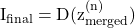
(22) $\begin{equation*}\mathrm{z_{merged}^{(j)} = z_{merged}^{(j-1)}\odot (1-M_{SAM,j}^{norm})+z_j \odot M_{SAM,j}^{norm}}\end{equation*}$

where z⁽⁰⁾_merged=z_bg,int, and the mask is broadcast across the C latent channels. After all subjects have been integrated, the merged latent is decoded:

(23) $\begin{equation*}\mathrm{I_{final} = D(z_{merged}^{(n)})}\end{equation*}$

Hyperparameters and Design Justifications

Table 1 summarizes all hyperparameters used across the various methods.

Parameter	Method(s)	Value	Justification
Object detection threshold (τ)	All	0.8	Balances detection recall vs. precision
Image downscaling factor	All (Stage 1)	0.25	Reduces VAE computation; 4×4 pooling
Fade radius (r_fade )	DOD-FADE, LOL-FADE	8% of min(w,h)	Empirically tuned for smooth transitions
Power exponent (p)	DOD-FADE, LOL-FADE	1.5	Matches perceptual smoothness; p<1 too soft
SAM dilation kernel (k)	DOD-SAM, LOL-SAM	5	Smooths mask boundaries; k=3 insufficient
Gaussian blur (σ)	DOD-SAM, LOL-SAM	3.0 pixels	Anti-aliasing for smooth transitions
VAE encoder stride	All	8	Standard SD v1.4; 512→64 resolution

Table 1 | Hyperparameters and design justifications for all four methods.

Algorithmic Summary and Pseudo-code

Algorithm 1 provides pseudo-code for LOL-SAM method, illustrating the complete pipeline.

Algorithm 1: Latent Object Layering with SAM Masking (LOL-SAM)

1:     procedure LOL-SAM(I,E,D,Detector,SAM)
2:     I_down ← Downscale(I, 0.25)
3:     z_bg ← E(I_down)
4:     z_bg,interp ← Bilinear(z_bg, size=(64,64))
5:     {B₁,…,B_n} ← Detector(I,τ=0.8)
6:     z_merged ← z_bg,interp
7:         for each B_j in {B₁,…,B_n} do
8:         I_j ← ExtractROI(I,B_j)
9:         z_j ← E(I_j)
10:         M_SAM,j ← SAM(I,B_j)
11:         M_latent ← Bilinear(M_SAM,j,(64,64))
12:         M_norm ← Normalize(M_latent,[0,1])
13:         z_merged ← z_merged · (1 – M_norm) + z_j · M_norm
14:     end for
15:     I_final ← D(z_merged)
16:     return I_final
17: end procedure

Styled Image Synthesis via LOL-SAM

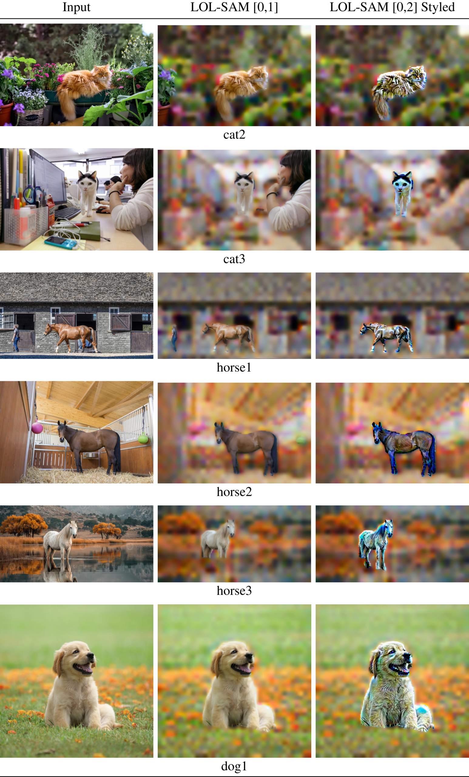
We evaluate LOL-SAM for stylized image synthesis from photographic inputs. The method combines object masking with latent-space manipulation to modify the selected object while retaining the surrounding background.

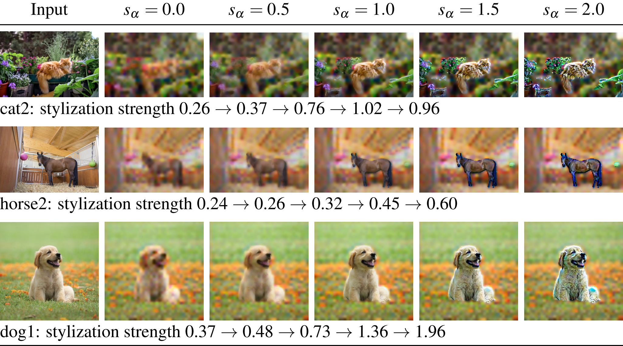
To examine how mask scaling affects the output, we conduct four controlled experiments. The quantitative results are shown in Tables 6 and 7, while visual comparisons are shown in Figures 2 and 3:

Mask-scale sweep: For each image, we changed the mask rescaling factor s_α using the values 0.0, 0.5, 1.0, 1.5, 2.0 and generated the corresponding outputs. We measured the stylization strength by calculating the relative increase in high-frequency energy in the subject region. We also recorded statistics of the latent values before decoding, including the mean, standard deviation, skewness, and the percentage of values outside the reference range.
Latent-value analysis: For each s_α, we recorded the distribution of latent values z_merged(c,u,ν) right before decoding. We calculated the percentage of values that were outside the reference latent range. As shown in Table 6, the variance of the latent values and the number of out-of-range values generally increased as s_α increased. These results support the hypothesis that latent saturation and clipping in the decoder may contribute to the stylized output.
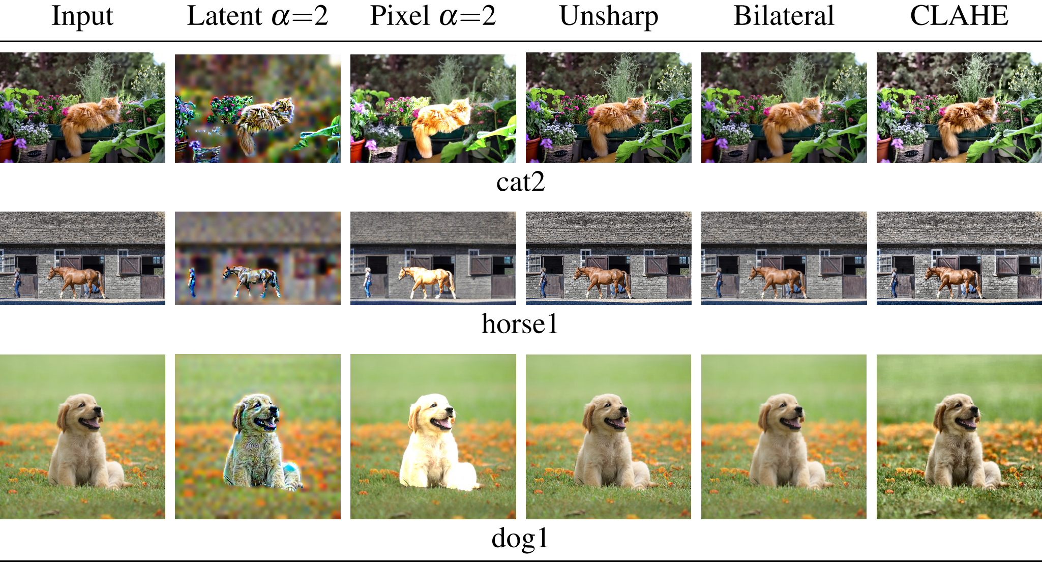
Pixel-space α > 1 control: To test whether similar stylization can be produced in pixel space, we scaled the RGB values in the subject region by s_α, kept the values within the valid pixel range, and used the same background compositing process. This increased the local contrast and saturation, but it also caused haloing and color-shift artifacts. These artifacts were different from those produced by latent rescaling, as shown in Table 6 and Figure 3.
Filter and baseline comparisons: We compared the stylized outputs to standard image-processing baselines, including unsharp masking, bilateral filtering, and CLAHE. These filters reproduce some aspects of the stylization, such as increased contrast and edge emphasis, but none of the individual baselines reproduce the full combination of texture, localized contrast amplification, and tonal compression observed with latent alpha extrapolation (Table 7).

Taken together, these experiments show that mask-alpha extrapolation changes the latent activation distribution, increasing latent activation magnitudes and producing values outside the range observed in standard reconstructions. These changes interact with the nonlinear VAE decoder and contribute to the resulting stylized appearance. The scripts used to reproduce these analyses are provided in the project repository²³.

Results

Benchmark and Evaluation Protocol

We evaluate all methods on a benchmark of 11 images covering four object classes: cars (3 images), cats (3 images), dogs (2 images), and horses (3 images). The complete image set and file names are available in the project repository²³. For reproducibility, we fix the seeds for all random components of the pipeline.

All four methods (DOD-FADE, DOD-SAM, LOL-FADE, LOL-SAM) use the same detection and prompt settings. SAM is called with multimask_output=false in the provided scripts. Exact command-line arguments and configuration details are provided in the project repository²³.

Metrics

We evaluate the results using FID, LPIPS, IoU, boundary error, and an aggregate score:

FID (ResNet-50 features): We compute the Fréchet distance from 2048-dimensional feature vectors extracted from the average-pooling layer of a pretrained ResNet-50, rather than the Inception-v3 network used in the standard FID formulation²⁶. We use ResNet-50 to maintain consistency with the detection backbone. These values are therefore not directly comparable with standard FID scores reported elsewhere. With only 11 images, the 2048-dimensional covariance estimates are not full-rank, and the resulting FID values have high sampling variance. We therefore interpret the reported values as directional rather than precise.
LPIPS: Learned Perceptual Image Patch Similarity computed using the VGG backbone over the foreground region. Lower values indicate greater perceptual similarity.
IoU: Intersection-over-Union between the method mask and an independent GrabCut reference segmentation. This measures agreement with the reference segmentation rather than accuracy against a known ground truth, since GrabCut itself is a semi-automatic method and may produce object boundaries that differ from those generated by SAM.
Boundary error (E): The RMSE (Root Mean Square Error) of differences in image gradients between the reconstructed and reference images within a band centered on the object boundary. Lower values indicate smaller gradient differences and smoother seam integration.
Aggregate composite score (Q_agg): We use a weighted aggregate score for summary reporting: $\mathrm{Q_{agg} = 0.5 \cdot (1-\tilde{E})+0.3⋅(1-\widetilde{FID}} )+ 0.2\cdot (1-\widetilde{LPIPS}})$ , where the tilde denotes min-max normalization to [0,1] across the evaluated set. Q_agg uses weights of 0.5, 0.3, 0.2 to boundary error, FID, and LPIPS, respectively. The per-image Q_”img” uses weights of 0.45, 0.35, 0.20 for edge quality, background smoothness, and object preservation. The two scores are not directly comparable.

Informal Human Comparison

We also conducted a blind visual comparison to see if our metric rankings matched human preferences. A small group of viewers examined unlabeled reconstruction pairs (Method A vs. Method B) and chose their preferred image. While limited in scale, the viewers’ preferences generally aligned with the Q_img rankings. A larger controlled study would be needed to confirm these results more rigorously (see Future Work).

Visual Presentation

For each test image, we provide a standardized three-panel presentation: original image (left), mask (SAM or FADE) (center), reconstruction (right). Below each panel, we include a compact numeric strip reporting: Q_img, IoU (when a reference mask is available), foreground LPIPS, and boundary error E. Full per-image raw outputs, metric logs, and plotting scripts are available in the project repository²³.

Quantitative Summary

Table 2 reports the mean values for each method. The results show different performance trade-offs between pixel-space (DOD) and latent-space (LOL) operations and between heuristic FADE and SAM-based masking. DOD methods obtain lower FID and foreground LPIPS, while LOL methods obtain lower boundary error. Among the four methods, DOD-SAM has the highest Q_agg score.

Method	FID	LPIPS (FG)	IoU	Boundary E	Q_agg
DOD-FADE	69.46	0.2425	0.3016	69.79	0.5000
DOD-SAM	71.79	0.2488	0.2457	64.45	0.5451
LOL-FADE	332.40	0.5776	0.3016	27.12	0.4459
LOL-SAM	354.86	0.6030	0.2457	17.53	0.5000

Table 2 | Mean quantitative results for the four reconstruction methods.

Analysis of Results

The four methods show different performance in terms of boundary quality and foreground fidelity:

RQ1 – Pixel vs. Latent Trade-offs (H1):

The pixel-space methods (DOD-FADE: Q_agg=0.5000, DOD-SAM: Q_agg = 0.5451) and latent-space methods (LOL-FADE: Q_agg =0.4459 , LOL-SAM: Q_agg = 05000) obtain relatively similar aggregate scores. The differences become more apparent when the individual metrics are considered. The DOD methods have lower FID values (≈71) and lower foreground LPIPS values (≈0.25), suggesting better preservation of the foreground. The LOL methods, on the other hand, have higher FID values (≈344) and higher LPIPS values (≈0.59), which indicates greater foreground distortion. The boundary-error results show the opposite trend. LOL-FADE and LOL-SAM have errors of 27.12 and 17.53, respectively, compared with approximately 67 for the DOD methods. The latent-space methods therefore produce smoother transitions around the object boundary, especially LOL-SAM. Overall, the results support H1: the latent-space methods improve boundary smoothness, but this improvement comes with some loss in foreground preservation.

RQ2 – Heuristic vs. Segmentation-Guided Masking (H2):

SAM-guided masks achieve lower IoU with GrabCut reference segmentations (IoU_SAM =0.2457) than the FADE heuristic masks (IoU_FADE =0.3016). Because GrabCut is a semi-automatic segmentation method rather than ground-truth annotation, the lower IoU primarily indicates disagreement between the two segmentation methods and does not necessarily imply inferior mask quality. The SAM-based methods also achieve lower boundary error in the latent space setting (LOL-SAM: E=17.53 vs. LOL-FADE: E=27.12). This represents a 35% reduction in boundary error and suggests that SAM-guided masking produces smoother boundary transitions after latent-space reconstruction. However, this reduction is smaller than the difference in boundary error observed between the pixel-space and latent-space methods overall. Taken together, the results provide partial support for H2. SAM-guided masking improves boundary quality within the latent-space settings, although the results do not show a corresponding improvement in foreground fidelity.

RQ3 – Synergistic Effects (H3):

Hypothesis H3 predicted that LOL-SAM would produce the highest composite quality as a result of the combined effects of latent-space blending and SAM masking. The overall results provide only partial support for this hypothesis. LOL-SAM has the lowest boundary error (E=17.53), but its foreground fidelity is substantially lower (LPIPS =0.6030), resulting in an aggregate quality score of Q_agg= 0.5000. This is comparable to DOD-FADE and does not establish a clear overall advantage for LOL-SAM. The per-image results in Table 3 are more favorable. LOL-SAM obtains the highest Q_img score on 9 of 11 images, indicating a stronger performance at the individual-image level than in the aggregate results. The higher FID and LPIPS values contribute to the lower aggregate score despite LOL-SAM having the lowest boundary error. Overall, the pixel-versus-latent representation has a stronger effect on aggregate quality, while SAM masking appears to improve performance within the latent-space methods on individual images.

Per-Image Evaluation: Composite Quality as the Appropriate Artistic Criterion

Per-Image Assessment Methodology

To evaluate the compositing quality of individual images, we tested all four methods using a custom three-part scoring system alongside standard metrics like FID and LPIPS. While standard metrics capture global image quality, our scoring system focuses on specific visual features that drive human perception: edge transition quality, background smoothness, and object preservation.

Edge Transition Quality (E): This metric is calculated in a narrow boundary region around the extracted object and evaluates how smoothly the gradients change across the object boundary. Lower values indicate smoother transitions between the foreground and the reconstructed background.
Background Smoothness (B): This metric is calculated over the reconstructed background region and measures how well extra high-frequency detail and remaining artifacts are reduced. It assigns higher scores to smoother reconstructed backgrounds rather than strictly preserving original sharp details. However, B may partly reflect the natural smoothing effect of the VAE in the LOL methods, so it may not be a completely independent measure of quality. Nonetheless, the weight sensitivity analysis shows that LOL-SAM remains competitive even when B is excluded. This is also true in the edge-only evaluation, where B has zero weight.
Object Preservation (O): Calculated using structural similarity, this metric compares the extracted foreground object to its corresponding region in the original image to measure how well the source details and appearance are preserved.

The overall per-image performance score was calculated as a weighted combination:

$\begin{equation*}\mathrm{Q_{img} = 0.45⋅E + 0.35\cdot B + 0.20\cdot O}\end{equation*}$

Edge transition quality was given the highest weight because boundary artifacts can be especially noticeable in image composites. For each test image, the method with the highest Q_img score was considered the best-performing method.

Per-Image Results

Table 3 shows the per-image composite quality scores for all 11 test images and four methods. The results reveal differences between the methods across individual images that are less clear in the aggregated metrics.

Image	DOD-FADE	DOD-SAM	LOL-FADE	LOL-SAM	Winner
car1.png	0.5371	0.5518	0.6622	0.6733	LOL-SAM
car2.png	0.4853	0.4788	0.6233	0.6225	LOL-FADE
car3.png	0.5563	0.5565	0.6743	0.6760	LOL-SAM
cat1.png	0.4670	0.4707	0.6391	0.6544	LOL-SAM
cat2.png	0.4802	0.5069	0.5029	0.6178	LOL-SAM
cat3.png	0.4844	0.4853	0.5663	0.6786	LOL-SAM
dog1.png	0.7134	0.7079	0.7962	0.7943	LOL-FADE
dog2.png	0.5428	0.5412	0.6359	0.6390	LOL-SAM
horse1.png	0.4270	0.4476	0.3430	0.4706	LOL-SAM
horse2.png	0.5236	0.5485	0.6319	0.7150	LOL-SAM
horse3.png	0.5160	0.5678	0.5313	0.6589	LOL-SAM

Table 3 | Per-image composite quality for each method across the test images.

Per-Image Analysis

LOL-SAM achieved the highest composite quality score on 9 of 11 test images (81.8%), while LOL-FADE outperformed the others on the remaining two. Neither DOD-FADE nor DOD-SAM secure the top score on any image. For LOL-SAM, the per-image scores range from 0.4706 to 0.7943, with a mean of 0.6546. The mean scores for LOL-FADE, DOD-SAM, and DOD-FADE are 0.6006, 0.5330, and 0.5212, respectively. Overall, these results demonstrate that LOL-SAM performs consistently across the test set.

Among the pixel-space methods, DOD-SAM has a higher mean score than DOD-FADE (0.5330 vs 0.5212) and scores higher on most of the test images. The difference between the two methods ranges from 0.0002 for car3 to 0.0518 for horse3. These images have more complex object boundaries, which suggests that the SAM-based mask may work better than the heuristic fade mask in these cases.

In an informal visual comparison, viewers generally preferred LOL-SAM over the other methods, consistent with the per-image Q_img rankings in Table 3. This suggests that Q_img correlates well with subjective human perception. However, a larger participant study is needed to establish statistical significance.

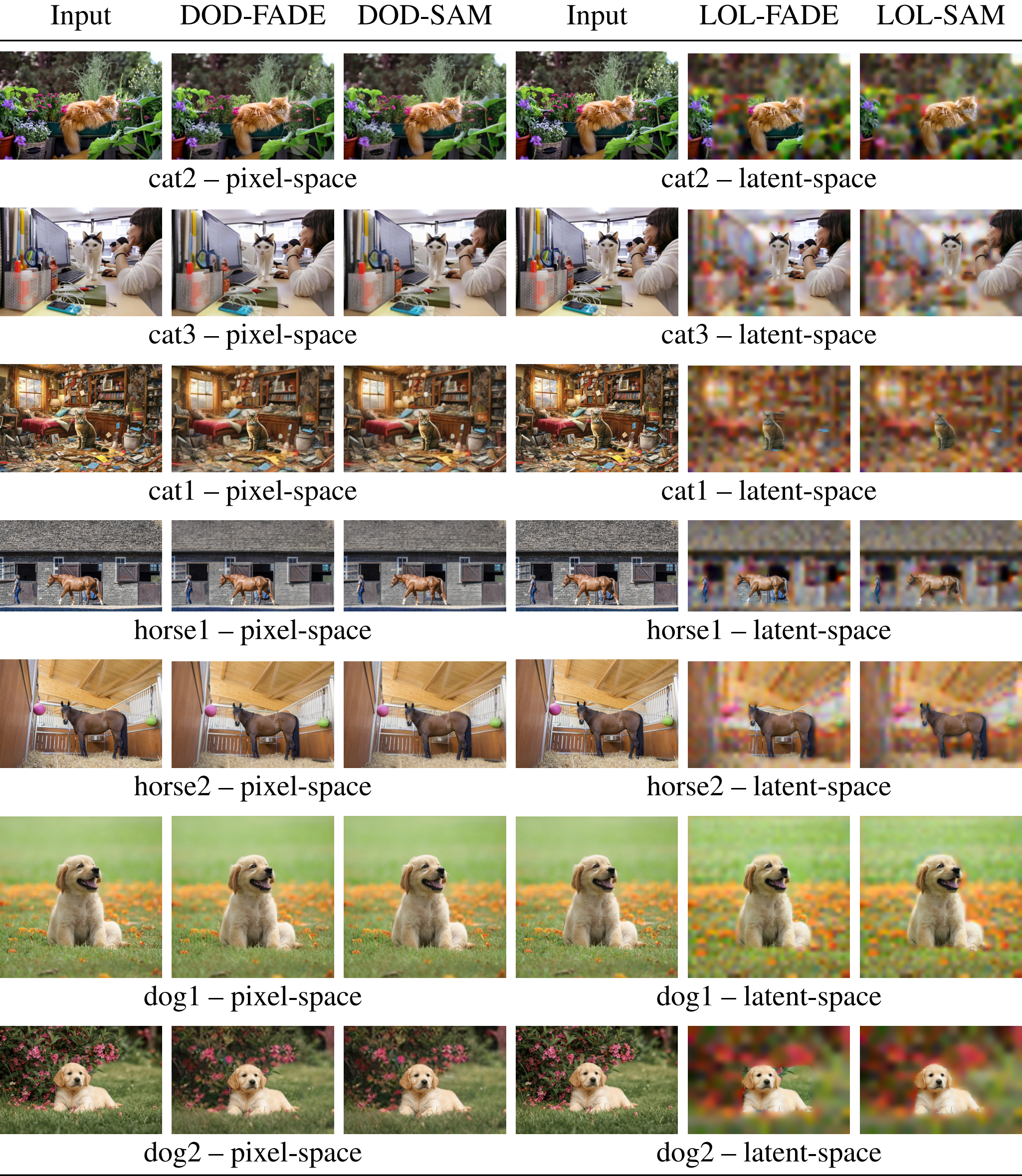
The qualitative results in Figure 4 reflect these differences. Overall, LOL-SAM produces more coherent composites with smoother boundary transitions. Conversely, in complex scenes like cat2 and horse1, the DOD methods exhibit noticeable boundary artifacts, such as haloing and color shifts. LOL-SAM’s latent-space blending, however, maintains smoother boundaries and achieves higher Q_img scores.

Composite Quality for Artistic Evaluation

These results show that traditional metrics, such as FID and LPIPS, do not always show clear differences between the methods when it comes to artistic quality. In comparison, the per-image quality score provides a more direct way to compare the methods in this evaluation. It combines three visual factors: edge smoothness (45%), background coherence (35%), and object preservation (20%). These factors are not directly measured by FID or LPIPS.

For artistic image reconstruction and object-aware editing, LOL-SAM performed better than the other methods tested. LOL-SAM had the highest per-image score on 9 of 11 images, which was also consistent with the preferences seen in the informal visual comparisons. It also had the lowest boundary error (E=17.53). Its results were consistent across the different object categories tested. Although LOL-SAM had higher FID and LPIPS values (approximately 355 and 0.60, respectively), it had a lower boundary error and higher per-image composite scores. This suggests that the latent-space approach may involve a trade-off between traditional technical metrics and the visual qualities measured by the composite score. For the artistic reconstruction setting studied here, the per-image composite quality score can provide additional information alongside overall metrics such as FID and LPIPS.

Human Preference Survey

We asked a small group of viewers to compare pairs of reconstructed images without telling them which method was used to create each image. The comparison included a subset of the 11 benchmark images. Viewers generally preferred LOL-SAM, which was consistent with the Q_img rankings in Table 3. However, only a few participants took part in the study, and the order of the images was not controlled. The sample was also too small to determine whether the relationship between Q_img and human preferences was statistically significant. These results provide some initial evidence that Q_img may be related to human visual preferences, but a larger and more controlled study would be needed to better examine this relationship.

Weight Sensitivity Analysis

We also tested whether the preference for LOL-SAM changes with the Q_img weighting scheme. We recomputed the per-image scores using three sets of weights: the original weights (0.45/0.35/0.20 for edge/smoothness/preservation), equal weights (1/3 each), and edge-only weighting (1.0/0/0). The results are presented in Tables 4 and 5.

Scheme	DOD-FADE	DOD-SAM	LOL-FADE	LOL-SAM
Original (0.45/0.35/0.20)	0.5212	0.5330	0.6006	0.6546
Equal (1/3 each)	0.5382	0.5444	0.5696	0.6111
Edge-only (1.0/0/0)	0.2755	0.3007	0.5997	0.7063

Table 4 | Weight sensitivity: mean Q_img across all 4 methods under alternative weighting schemes.

Scheme	DOD-FADE	DOD-SAM	LOL-FADE	LOL-SAM
Original	0/11	0/11	2/11	9/11
Equal	0/11	1/11	2/11	8/11
Edge-only	0/11	0/11	2/11	9/11

Table 5 | Weight sensitivity: per-image win counts (best Q_img on each image) under alternative weighting schemes.

The method ranking LOL-SAM > LOL-FADE > DOD-SAM > DOD-FADE is the same under all three weighting schemes. LOL-SAM has the highest score on 8–9 of 11 images, depending on the weighting scheme, and its mean-score advantage over LOL-FADE increases from 0.054 under the original weighting to 0.107 with edge-only weighting. Under edge-only weighting, the DOD methods have near-zero edge scores, while their scores are higher under the original weighting. This indicates that foreground preservation contributes more to their original Q_agg scores than boundary quality. Overall, the method ranking is not sensitive to the weighting schema that was tested.

Applications: Styled Image Synthesis

Stylized Outputs

Using the mask-alpha extrapolation described in the Methods section, M_stylized=2.0 ⋅ M_SAM^norm, Figure 1 shows the resulting stylized outputs. The subjects exhibit high-contrast brush-stroke textures resembling an oil-painting style, while the backgrounds retain smooth, gradual color transitions. These examples demonstrate that the LOL-SAM framework can also support object-aware artistic stylization in addition to image reconstruction.

Stylization Effects via Extended Latent Masking

Figure 1 | Stylization effects via extended latent mask scaling. Each row displays the original input image, LOL-SAM reconstruction with normal mask scaling [0,1], and extended mask scaling [0,2]. Extended scaling induces artistic brush-stroke textures and tonal compression on the subject region.

Stylization Ablation Results

We evaluated the stylization effect using controlled ablation experiments on all 11 benchmark images. Three patterns were observed: (1) the latent statistics change consistently with the mask-scale factor, (2) pixel-space scaling produces different visual artifacts, and (3) standard filters do not produce the same localized stylization effect.

Latent Activation Statistics Across Mask-Scale Factors

Table 6 shows the latent activation statistics recorded immediately before decoding, averaged across all 11 images. As the mask-scale factor s_α increases from 0.0 to 2.0, the latent standard deviation increases monotonically from 3.163 to 3.836, while the fraction of activations exceeding the reference |z|>1 range increases from 76.4% to 78.0%. The range of extreme values (minimum and maximum) also expands substantially. Thus, increasing the mask-scale factor produces greater variation in the latent activations and places more activations outside the reference range. This change may contribute to the observed stylization, potentially through the nonlinear response of the VAE decoder to these latent values.

s_α	Latent Std	\|z\|>1 (%)	\|z\|>3 (%)	Styliz. Strength	Q_img
0.0	3.163	76.4	37.1	0.295	0.692
0.5	3.154	76.4	37.2	0.333	0.679
1.0	3.276	77.1	38.5	0.458	0.641
1.5	3.511	77.6	39.8	0.653	0.588
2.0	3.836	78.0	40.8	0.736	0.558

Table 6 | Latent activation statistics vs. mask-scale factor s_α (mean across 11 images). Monotonic increase in std and out-of-range fraction confirms decoder saturation as the mechanism driving stylization.

Pixel-Space and Filter Control Comparisons

Table 7 compares latent-space mask extrapolation with pixel-space alpha scaling and standard image filters. Two main differences are observed:

Pixel-space α > 1 produces weaker stylization: Pixel-space scaling at s_α=1.5 produces a stylization strength of 0.409, decreasing slightly to 0.399 at s_α=2.0. In comparison, latent-space scaling increases from 0.653 at s_α=1.5 to 0.736 at s_α=2.0. Simple RGB scaling therefore does not produce the same stylization effect as latent-space operations.
Filters operate globally, not locally: Unsharp masking (1.477) and CLAHE (1.591) achieve high stylization strength values, but they enhance high-frequency energy across the entire image rather than selectively within the object region. Both filters also produce lower edge blending scores (0.032 and 0.026 respectively) than latent methods (0.513–0.784), as well as lower background smoothness scores (0.421 and 0.365 vs. 0.734–0.750). These results indicate that they do not reproduce the object-aware stylization observed with latent alpha extrapolation.

Method	Edge	Smooth	Obj. Pres.	Q_img	Styliz.
Latent α = 1.0	0.681	0.734	0.387	0.641	0.458
Latent α = 1.5	0.579	0.726	0.368	0.588	0.653
Latent α = 2.0	0.513	0.734	0.350	0.558	0.736
Pixel α = 1.5	0.260	0.846	0.441	0.501	0.409
Pixel α = 2.0	0.255	0.840	0.428	0.494	0.399
Unsharp mask	0.032	0.421	0.954	0.353	1.477
Bilateral filter	0.137	0.675	0.885	0.475	0.554
CLAHE	0.026	0.365	0.862	0.312	1.591

Table 7 | Comparison of latent-space mask extrapolation vs. pixel-space controls and filter baselines (mean across 11 images).

Mask-Scale Sweep: Visual Comparison

Figure 2 shows a mask-scale sweep for two images from different object categories. As s_α increases, the subject region shows progressively stronger brush-stroke texture and tonal compression, while the background remains smooth. The stylization effect remains localized to the subject region and increases as the mask-scale factor increases.

Figure 2 | Mask-scale sweep across s_α ∈ {0.0,0.5,1.0,1.5,2.0}.. Progressive increase in s_α produces progressively stronger stylization (brush-stroke texture, tonal compression) localized to the subject region. Per-image stylization strength values (foreground Laplacian energy ratio vs. original) are reported below each row.

Pixel-Space vs. Latent-Space Control: Visual Comparison

Figure 3 shows the visual outputs of latent-space mask extrapolation (s_α = 2.0), pixel-space alpha scaling (s_α = 2.0), and the three filter baselines. Latent-space extrapolation creates localized brush-stroke stylization on the subject while keeping the background smooth. Pixel-space scaling increases the overall brightness and produces haloing around object boundaries, but does not produce the localized brush-stroke texture seen with the latent method. In contrast, the filter baselines apply their effects globally, altering both the object and background rather than isolating the subject.

Figure 3 | Comparison of latent-space mask extrapolation (s_α = 2.0) with pixel-space alpha scaling and standard image filters.

Qualitative Comparison: Pixel-Space vs. Latent-Space Methods

Figure 4 shows side-by-side comparisons of the four methods using selected benchmark images. The pixel-space methods (DOD-FADE and DOD-SAM) preserve more details in the foreground, but they also exhibit visible boundary artifacts, such as sharp edges and color shifts. The latent-space methods (LOL-FADE and LOL-SAM) produce smoother transitions around the object, but some foreground texture is lost. Within each group, the visual difference between FADE and SAM masks is relatively small, which is consistent with their similar Q_img scores in Table 3. In the pixel-space methods, both masks cover most of the ROI, with the main differences occurring near the object boundaries. The project repository²³ contains the per-image raw outputs, metric logs, and plotting scripts used in the analysis.

Discussion

Key Findings and What We Learned

The results show a trade-off between preserving the foreground object and improving boundary quality in object-aware image reconstruction. The pixel-space methods (DOD) preserve more foreground detail (LPIPS ≈0.25) but produce sharper boundaries and higher gradient discontinuity (E≈67). The latent-space methods (LOL) produce smoother boundary transitions (E≈22), but with greater foreground distortion (LPIPS ≈0.59). In the aggregate score Q_agg ,these differences result in relatively similar overall scores: DOD-SAM leads slightly at 0.5451, DOD-FADE and LOL-SAM tie at 0.5000, and LOL-FADE scores 0.4459. Thus, the lower boundary error of the LOL methods partly offsets their higher FID and LPIPS values.

Within each domain, SAM-guided masks generally outperform the heuristic FADE masks. In latent space, LOL-SAM reduces the boundary error from 27.12 to 17.53 relative to LOL-FADE, with a Q_agg difference of 0.054. In pixel space, DOD-SAM also outperforms DOD-FADE, with a Q_agg difference of 0.045. The largest per-image differences occur on horse3, cat2 and horse2, which have relatively complex object boundaries. These results indicate that the masking strategy affects performance, although the choice between pixel- and latent-space processing has a larger effect.

The per-image scores provide a different ranking from the aggregate scores. LOL-SAM has the highest Q_img on 9 of 11 test images (81.8%), with an average score of 0.6546. The corresponding averages are 0.6006 for LOL-FADE, 0.5330 for DOD-SAM, and 0.5212 for DOD-FADE. LOL-SAM has the highest score on all three cat images, all three horse images, and two of the three car images. Neither DOD method has the highest score on any image. The difference between the aggregate and per-image rankings indicates that averaging across images can mask differences in performance, particularly when boundary quality has greater weight in the evaluation.

The informal human comparisons also favored LOL-SAM, consistent with the Q_img rankings in Table 3. The metric assigns 45% weight to edge transition, 35% to background coherence, and 20% to foreground preservation. However, the small sample size and uncontrolled presentation order preclude establishing a statistically significant relationship between Q_img and human preference.

Limitations

Dataset scale: The benchmark contains only 11 images across four object classes limiting how well the results can be generalized to larger and more diverse datasets with varied lighting and complex compositions.
Segmentation dependency: The pipeline lacks automated quality checks for detection or masking. Failures of Faster R-CNN on occluded or atypical objects, as well as SAM mask degradation (leakage or under-segmentation), can propagate to the compositing results.
Latent-space resolution: The VAE’s 8× spatial compression (512 x 512 → 64 x 64) limits fine-detail preservation, while unconstrained latent distributions during blending may produce decoder saturation artifacts.
Metric robustness: Although the weight-sensitivity analysis (Tables 4–5) shows stable method rankings, the composite quality weights and individual metrics have yet to be validated against large-scale human preference data.
Computational cost: Synchronous per-ROI SAM inference scales with the number of objects, and wall-clock latency and memory consumption across methods are not reported.
Mask heuristics: The FADE mask uses fixed parameters (r_fade = 8%, p = 1.5) and does not adapt to object shape or aspect ratio.
Scope: This work focuses on artistic compositing and does not evaluate photorealism preservation, color-accurate blending, or physics-based boundary lighting. The method has not been evaluated on other compositing tasks.

Implications for Artistic Application

For artistic image reconstruction, LOL-SAM is well suited to applications where visual coherence and smooth boundary integration are important. Although LOL-SAM has higher FID and LPIPS values, it achieves lower boundary error and higher per-image scores. For the reconstruction setting evaluated here, this trade-off may be acceptable when boundary quality and overall visual integration are prioritized. The results also show that FID and LPIPS alone do not fully reflect the qualities emphasized in image compositing, supporting the use of evaluation measures that account for boundary quality and visual integration.

Future Work

Learned blending and masking: Train models to learn adaptive per-pixel blend weights in latent space and replace the heuristic FADE masks with learned interpolation networks optimized for boundary quality.
Hybrid latent-pixel architectures: Perform the initial blending in latent space to improve global coherence, then refine boundaries with pixel-space operations at an intermediate resolution before decoding.
Broader evaluation: Expand the benchmark to more than 100 images covering a wider range of object categories and conduct more experiments to see how changes in weights affect the results.
Perceptual validation: Conduct a larger human preference study with both general and expert participants, controlled presentation order, agreement measures such as Krippendorff’s α, and preference margins. This would provide a better comparison between Q_img and human judgments.
Task-specific metrics: Develop compositing metrics for photorealism, color consistency, and physical plausibility to extend the evaluation beyond artistic applications.

Figure 4 | Qualitative comparison of all object categories. Left three columns: pixel-space methods (Input/DOD-FADE/DOD-SAM); right three: latent-space methods (Input/LOL-FADE/LOL-SAM). The latent-space methods produce smoother boundary blending but can cause more distortion in the foreground object. Full results for all 11 benchmark images are available in the project repository²³.

Acknowledgements

I would like to sincerely thank Professor Greg Shakhnarovich for his mentorship and guidance throughout the past year. His detailed explanations and patient support with research methods, coding, and comparing generated images were very helpful to this project. I would also like to thank my high school computer science and mathematics teachers for giving me the knowledge and encouragement to pursue independent research. Finally, I am grateful to the anonymous reviewers for their helpful feedback, which help improve this paper. I appreciate everyone who supported me and helped me grow as a student and researcher.

References

R. Rombach, A. Blattmann, D. Lorenz, P. Esser, B. Ommer. High-resolution image synthesis with latent diffusion models. Proceedings of the IEEE/CVF Conference on Computer Vision and Pattern Recognition, 10684–10695 (2022). [↩] [↩] [↩]
A. Kirillov, E. Mintun, N. Ravi, H. Mao, C. Rolland, L. Gustafson, T. Xiao, S. Whitehead, A. C. Berg, W.-Y. Lo, P. Dollár, R. Girshick. Segment Anything. Proceedings of the IEEE/CVF International Conference on Computer Vision, 4015–4026 (2023). [↩] [↩] [↩] [↩] [↩]
J. Ho, A. Jain, P. Abbeel. Denoising diffusion probabilistic models. Advances in Neural Information Processing Systems 33, 6840–6851 (2020). [↩]
J. Song, C. Meng, S. Ermon. Denoising diffusion implicit models. International Conference on Learning Representations (2021). [↩]
P. Dhariwal, A. Nichol. Diffusion models beat GANs on image synthesis. Advances in Neural Information Processing Systems 34, 8780–8794 (2021). [↩]
A. Ramesh, P. Dhariwal, A. Nichol, C. Chu, M. Chen. Hierarchical text-conditional image generation with CLIP latents. arXiv (2022). [↩]
C. Saharia, W. Chan, S. Saxena, L. Li, J. Whang, E. Denton, S. K. S. Ghasemipour, R. Gontijo Lopes, B. Karagol Ayan, T. Salimans, J. Ho, D. J. Fleet, M. Norouzi. Photorealistic text-to-image diffusion models with deep language understanding. Advances in Neural Information Processing Systems 35 (2022). [↩]
A. Radford, J. W. Kim, C. Hallacy, A. Ramesh, G. Goh, S. Agarwal, G. Sastry, A. Askell, P. Mishkin, J. Clark, G. Krueger, I. Sutskever. Learning transferable visual models from natural language supervision. Proceedings of the 38th International Conference on Machine Learning 139, 8748–8763 (2021). [↩]
A. Nichol, P. Dhariwal, A. Ramesh, P. Shyam, P. Mishkin, B. McGrew, I. Sutskever, M. Chen. GLIDE: Towards photorealistic image generation and editing with text-guided diffusion models. arXiv (2022). [↩]
A. Hertz, R. Mokady, J. Tenenbaum, K. Aberman, Y. Pritch, D. Cohen-Or. Prompt-to-Prompt image editing with cross-attention control. Proceedings of the IEEE/CVF International Conference on Computer Vision, 14136–14146 (2023). [↩]
G. Couairon, J. Verbeek, H. Schwenk, M. Cord. DiffEdit: Diffusion-based semantic image editing with mask guidance. International Conference on Learning Representations (2023). [↩]
O. Avrahami, D. Lischinski, O. Fried. Blended diffusion for text-driven editing of natural images. Proceedings of the IEEE/CVF Conference on Computer Vision and Pattern Recognition, 18208–18218 (2022). [↩]
R. Mokady, A. Hertz, K. Aberman, Y. Pritch, D. Cohen-Or. Null-text inversion for editing real images using guided diffusion models. Proceedings of the IEEE/CVF Conference on Computer Vision and Pattern Recognition, 6038–6047 (2023). [↩]
L. Zhang, A. Rao, M. Agrawala. Adding conditional control to text-to-image diffusion models. Proceedings of the IEEE/CVF International Conference on Computer Vision, 3836–3847 (2023). [↩]
Y. Li, H. Liu, Q. Wu, F. Mu, J. Yang, J. Gao, C. Li, Y. J. Lee. GLIGEN: Open-set grounded text-to-image generation. Proceedings of the IEEE/CVF Conference on Computer Vision and Pattern Recognition, 22511–22521 (2023). [↩]
O. Bar-Tal, D. Ofri-Amar, R. Fridman, Y. Kasten, T. Dekel. Text2LIVE: Text-driven layered image and video editing. European Conference on Computer Vision 13688, 707–723 (2022). [↩]
J. Johnson, A. Alahi, L. Fei-Fei. Perceptual losses for real-time style transfer and super-resolution. European Conference on Computer Vision 9906, 694–711 (2016). [↩]
D. Ulyanov, A. Vedaldi, V. Lempitsky. Instance normalization: The missing ingredient for fast stylization. arXiv (2017). [↩]
S. Ren, K. He, R. Girshick, J. Sun. Faster R-CNN: Towards real-time object detection with region proposal networks. Advances in Neural Information Processing Systems 28 (2015). [↩]
J. Long, E. Shelhamer, T. Darrell. Fully convolutional networks for semantic segmentation. Proceedings of the IEEE Conference on Computer Vision and Pattern Recognition, 3431–3440 (2015). [↩]
K. He, G. Gkioxari, P. Dollár, R. Girshick. Mask R-CNN. Proceedings of the IEEE International Conference on Computer Vision, 2961–2969 (2017). [↩]
L.-C. Chen, G. Papandreou, I. Kokkinos, K. Murphy, A. L. Yuille. Semantic image segmentation with deep convolutional nets and fully connected CRFs. International Conference on Learning Representations (2015). [↩]
O. Tong, G. Shakhnarovich. Object-aware image reconstruction: Code and implementation. Technical Report (2026). GitHub: https://github.com/penguin12b5/latent_space_image_manager. [↩] [↩] [↩] [↩] [↩] [↩] [↩] [↩] [↩]
D. P. Kingma, M. Welling. Auto-encoding variational Bayes. arXiv (2014). [↩]
T.-Y. Lin, M. Maire, S. Belongie, L. Bourdev, R. Girshick, J. Hays, P. Perona, D. Ramanan, C. L. Zitnick, P. Dollár. Microsoft COCO: Common objects in context. European Conference on Computer Vision 8693, 740–755 (2014). [↩]
M. Heusel, H. Ramsauer, T. Unterthiner, B. Nessler, S. Hochreiter. GANs trained by a two time-scale update rule converge to a local Nash equilibrium. Advances in Neural Information Processing Systems 30 (2017). [↩]