When Perfect Is Wrong: Exposing the AUC ≈ 1.0 Illusion in Chronic Kidney Disease Machine Learning Benchmarks

Abstract

Chronic kidney disease (CKD) is a serious progressive condition, but many machine-learning studies continue to use the University of California, Irvine (UCI) CKD dataset (n=400), and yield area-under-the-curve (AUC) values near 1.0. We investigated whether the results on UCI reflect strong algorithms or a ceiling effect limiting model comparison. We studied three datasets representing different tasks: the UCI CKD, the National Health and Nutrition Examination Survey (NHANES) 2021-2023, and the Tawam Hospital UAE cohort. We evaluated 5 models using stratified training-test splits, repeated learning curves, single-feature screening, staged feature removal, training-test performance comparisons, and cross-dataset evaluation. For preprocessing, we used training data only for missing-value imputation and scaling, with each learning curve point generated from 20 repeated subsamples. UCI-trained models generated AUC values near 1.0 with small training samples. NHANES performance declined after feature ablation: first with the removal of estimated glomerular filtration rate (eGFR) and albumin-to-creatinine ratio (ACR), then again after removing creatinine and blood urea nitrogen (BUN). The performance decline was attributed to the removal of the measurements defining CKD status and markers of kidney function. Tawam produced lower AUC values compared to UCI, with performance improving with training size. We then performed a cross-dataset evaluation of UCI-trained models on NHANES and Tawam using three shared features. We found that UCI-trained models yielded lower and more varied AUC values when applied to NHANES and Tawam. These results suggest that UCI remains useful as a teaching and code validation dataset, but remains limited for model comparison and clinical usage.

Keywords: chronic kidney disease, machine learning, AUC, benchmark validity, learning curves, clinical informatics, shortcut learning, cross-dataset validation

Introduction

Background and Context

Nearly 700 million people globally have chronic kidney disease¹. Because early-stage CKD is often asymptomatic, early diagnosis is challenging. This leads many patients to receive diagnosis only after developing significant declines in kidney function². At this advanced stage, treatment options may include dialysis or transplantation, both of which create challenges for patients and healthcare systems². Due to this clinical gap, extensive work on automated CKD recognition has occurred, primarily through routine laboratory and demographic data^3,4,5,6,7. In the published machine-learning literature, however, one benchmark dominates: the UCI CKD dataset⁸. Previous research using UCI frequently reported near-perfect performance across several models^9,4,10. This raises questions regarding whether these results reflect strong model performance or weak benchmarks unable to compare between them.

Benchmark Validity

Useful benchmarks should distinguish competing methods. When different models produce similar results, benchmarks struggle to determine which method is best. Additionally, it must represent the clinical task for which the model is intended. Reporting guidelines emphasize transparent outcome definitions, validation, calibration, and considerations of model transportability¹¹. Shortcut learning illustrates these concerns. For example, Zech et al. found that a pneumonia model relied partly on hospital- and scanner-specific features, leading to a performance decline when evaluated at other hospitals¹². Other related shortcut and transportability issues have been reported elsewhere^13,14,15.

Problems regarding model comparison matter because the UCI, NHANES, and Tawam datasets have fundamentally different tasks. UCI primarily represents Indian hospital records and patients with labeled CKD. Rather than detect early-stage CKD, it tests whether the models can recognize already labeled CKD. NHANES classifies CKD at one point in time. Some variables used to determine CKD status can also be given to the model as predictors. Tawam includes high-cardiovascular-risk patients in Abu Dhabi who began with relatively preserved kidney function and received follow-ups to track CKD progression¹⁶. The datasets differ in their patients, outcomes, and CKD rates, which means that their scores cannot be directly compared. This paper therefore treats them as separate case studies.

Study Objectives

This study evaluates whether the strong performance often reported on UCI is a property of strong algorithms or of an unusually easy benchmark. The analysis uses cross-dataset evaluation, three NHANES feature sets, stratified repeated learning curves, UCI categorical preprocessing, UCI ablation, Tawam overfitting checks, Brier and threshold summaries, and a KDIGO stage mapping.

Methods

Datasets

Dataset	N	Origin	CKD label	Key features
UCI CKD	400	India hospital EHR	CKD/not-CKD class	Hemoglobin, specific gravity, creatinine, packed cell volume, albumin
NHANES 2021–2023	11,933	U.S. national health survey	eGFR <60 or ACR ≥ 30	Creatinine, BUN, albumin, BMI, eGFR, ACR, diabetes, blood pressure
Tawam Hospital UAE	491	Abu Dhabi EHR	9-year CKD incidence	Creatinine, eGFR, HbA1c, cholesterol, triglycerides, blood pressure, BMI

Dataset	CKD stages represented	Stages excluded	Population setting
UCI CKD	Not directly determined	Not directly determined	Hospital records
NHANES 2021–2023	G1–G5 by eGFR/ACR criteria	None by definition	U.S. community-dwelling sample
Tawam Hospital UAE	Baseline G1–G2; progression toward G3a-G5	G3–G5 at baseline excluded	Hospital outpatient cohort

Dataset	N	Pos.	Pos. rate	Pred.	Miss.	Train N	Train pos.	Test N	Test pos.	Dup. IDs
UCI CKD	400	250	0.625	24	1,012	300	0.627	100	0.620	N/A
NHANES 2021–2023	11,933	8,341	0.699	11	38,655	10,143	0.699	1,790	0.699	0
Tawam UAE	491	56	0.114	10	21	368	0.114	123	0.114	0

We chose the existing NHANES 2021-2023 cohort instead of rebuilding it from the original NHANES files. The 2021-2023 cohort already had columns with eGFR, albumin-creatinine ratio, CKD stage, and CKD status. Since the 2021-2023 cohort already contained eGFR values, we decided not to recreate them using creatinine; this is why the modeling script does not specify the equation used to calculate eGFR. The only participants that we retained were those with a recorded CKD label. We did not remove participants from the analysis for missing predictor values, and missing values were filled in only using information from training data. Before imputation, the resulting file contained 11,933 participants, 8,341 CKD-positive labels, 11 predictors, and 38,655 missing predictor cells. Since the purpose of the study is to examine model behavior instead of creating a nationally representative CKD estimate, we did not use NHANES survey weights or sampling-design variables. Additionally, CDC/NCHS notes that the sampling design changed specifically for the 2021-2023 cohort, so the unweighted results should not be interpreted as nationally representative¹⁹.

NHANES and UCI also contain different predictors. For example, UCI contains hemoglobin and urine specific gravity, whereas NHANES includes BMI and diabetes status. Differences in results may reflect different prediction tasks and available information. Therefore, the two dataset’s results should not serve as evidence that one patient population is easier to classify

Preprocessing

Before modeling, we divided each dataset into training and test groups, both containing around the same proportions of negative and positive outcomes. Imputation of missing data came from training data only. If there were missing numerical values, we replaced them with the median. Missing categorical values were replaced with the most common category. Small datasets are particularly susceptible to validation performance inflation when test group information influences model preparation²⁰. As a precaution, we standardized numerical predictors using only training data, then applied the same parameters to the test data. UCI variables without natural rankings were one-hot-encoded. Any variables with meaningful clinical order, such as urine specific gravity and urine dipstick measurements, were encoded to preserve their order. For Tawam, we retained selected baseline predictors, excluding participant identifiers and follow-up time. We also checked the StudyID column for any duplicate identifiers that could appear in both training and test sets and found none.

Ethical Considerations

This study analyzed de-identified public or previously existing datasets and did not recruit, contact, or intervene with patients. The UCI CKD is publicly available through the UCI Machine Learning Repository that supports reuse, permitting attribution⁸. NHANES was released by the CDC/NCHS under its public-use data procedures¹⁷. The Tawam data cohort accompanies a published study that reported local ethics approval¹⁶. Therefore, the present manuscript did not require the author to obtain new institutional review board approval or obtain additional informed consent.

Models and Experiments

Model	Family	Key hyperparameters	Role
Logistic Regression	Linear	C=1.0, max_iter=1000	Interpretable baseline
Random Forest	Bagging ensemble	200 trees, depth 8, minimum leaf 5	Nonlinear baseline
Histogram Gradient Boosting	Boosting ensemble	300 iterations, learning rate 0.05, depth 5, minimum leaf 20	Primary learning-curve model
Neural Network (MLP)	Deep learning	128–64–32 hidden units, early stopping, 500 iterations	Flexible nonlinear model
Soft-voting Ensemble	HGB + RF + MLP	Soft voting over three base learners	Aggregate benchmark

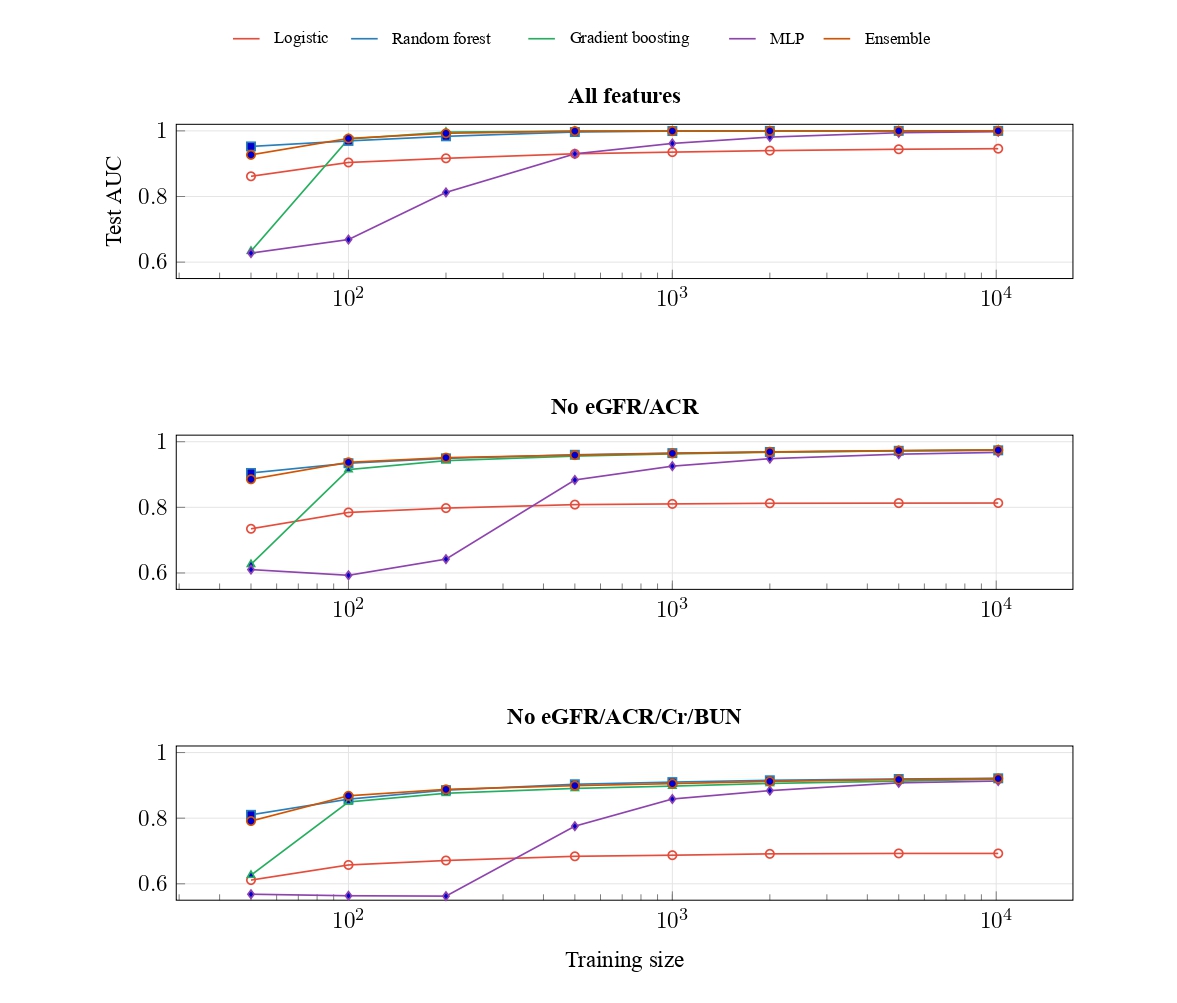
Our analysis also contained seven complementary experiments. First, we trained all five models using the available training data, then used them to generate predictions on the test data, and compared their performance. We then used learning curves to measure performance changes as the training size increased. We evaluated NHANES using three predictor sets: all predictors; all predictors except eGFR and ACR; and all predictors except eGFR, ACR, creatinine, and BUN. Comparing the predictor sets quantified changes in model performance when removing kidney-related predictors. For UCI, we screened the predictors individually, then retrained the models after removing the three strongest predictors. On Tawam, we compared training and test performance to assess the possibility of overfitting. Finally, we evaluated UCI-trained models without retraining on NHANES and Tawam using three shared variables: age, systolic blood pressure, and serum creatinine. We used seed 42 for primary training and test splits for data partition reproduction. We also ran repeated subsampling experiments with different predetermined seeds for the same purpose. We measured model discrimination through area under the receiver operating characteristic curve (AUC-ROC, abbreviated as AUC in the tables). In order to provide additional information beyond AUC, we calculated Brier scores for both NHANES and Tawam. We also calculated model specificity and sensitivity at a threshold of 0.5. However, neither Brier scores, AUC values, nor specificity and sensitivity demonstrate whether using the models’ predicted probabilities of CKD-positive outcomes would improve clinical decisions¹¹.

Power-Law Fits

NHANES learning curves are summarized by an inverse power-law equation, which describes how model performance changes with sample size^21,22:

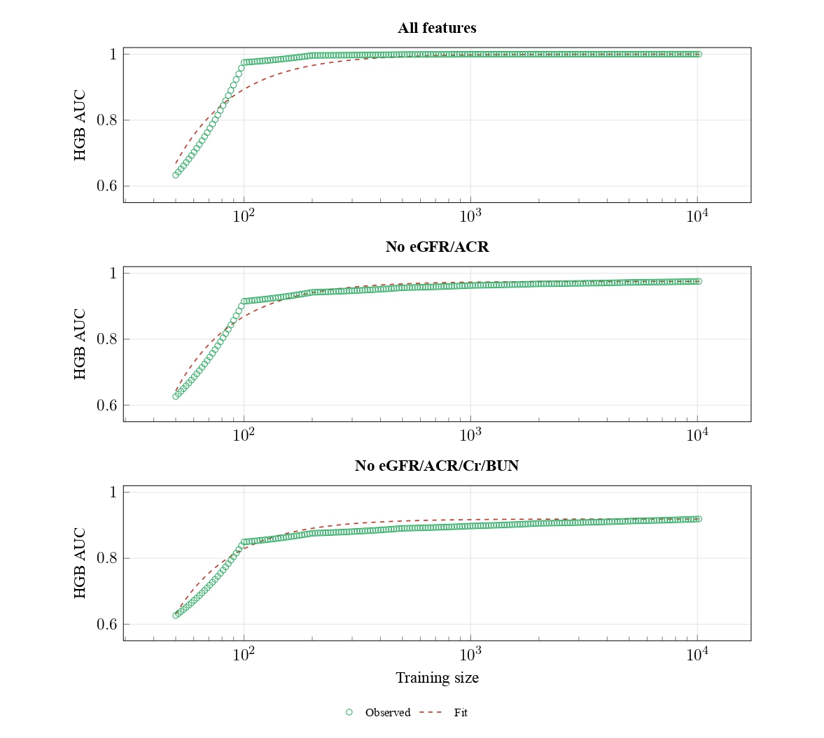
The fitted ceiling, c, could not fall below the maximum observed AUC or exceed the maximum possible AUC value of 1.0. If the model had an observed AUC of 1.0, it meant that the model had perfectly ranked all positive cases above all negative cases in the particular test sample. Since 1.0 is also the maximum possible AUC value, we therefore placed the lower limit just below 1.0 to give the program a range to estimate the ceiling.  We constrained parameter a, which controls the size of the gap below the fitted ceiling, from 0 to 200 and b, which controls how the gap changes with training size, from 0 to 5. We began the fitting process with c = min(1.0, max(AUC) + 0.01), a = 2.0, b = 0.5, with the program adjusting the parameters to minimize the squared difference between the fitted curve and observed AUC values. In order to estimate the stability of the fitted parameters, we used 500 bootstrap resamples of the learning-curve points, with Table 8 reporting the middle 95% of the resulting parameter estimates as bootstrap intervals. We also removed the two smallest training sizes, then refitted the curve to see whether the estimated ceiling depended on results from small samples. The curves summarize how performance changed for each model and NHANES predictor set. Therefore, conclusions should be limited to the tested models, predictor sets, and NHANES sample examined here. The power law curves provide an estimated ceiling; however, such a ceiling is neither a biological limit on CKD prediction nor a guarantee of future performance. Likewise, a reported value of c=1.000 or a=200 indicates that the ceiling reached its upper boundary or the scale parameter reached its boundary, respectively. In either case, the data produced an uncertain, imprecise parameter estimate rather than a precise estimate.

Results

Full-Data Comparison

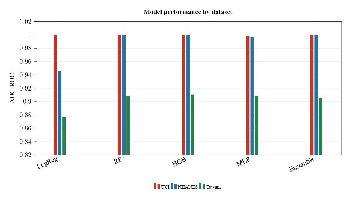
Model	UCI AUC	NHANES AUC	Tawam AUC	NHANES Brier	Tawam Brier
LogReg	1.0000	0.9457	0.8768	0.0835	0.0612
RF	0.9996	1.0000	0.9083	0.0043	0.0658
HGB	1.0000	1.0000	0.9102	0.0001	0.0576
MLP	0.9983	0.9971	0.9083	0.0153	0.1397
Ensemble	1.0000	1.0000	0.9050	0.0033	0.0663

Model	Dataset	Sensitivity	Specificity
LogReg	NHANES	0.963	0.742
LogReg	Tawam	0.357	1.000
RF	NHANES	1.000	1.000
RF	Tawam	0.143	1.000
HGB	NHANES	1.000	1.000
HGB	Tawam	0.429	0.982
MLP	NHANES	0.989	0.961
MLP	Tawam	0.786	0.917
Ensemble	NHANES	1.000	1.000
Ensemble	Tawam	0.286	1.000

Learning Curves

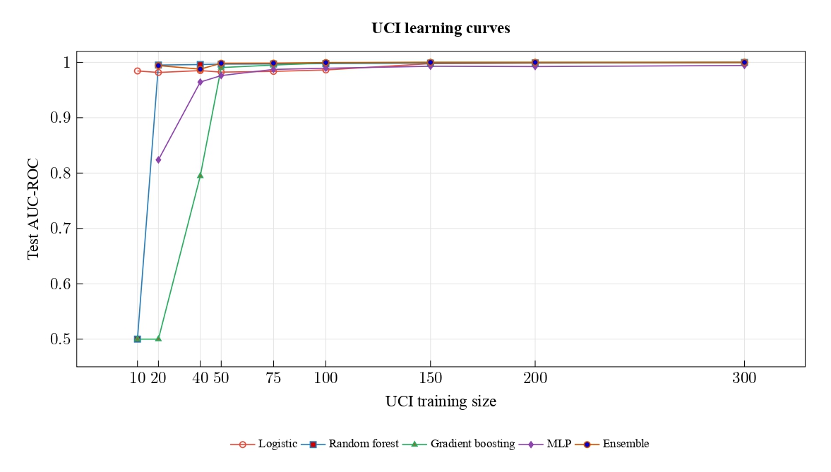
UCI learning curves plateau rapidly. Across repeated samples, gradient boosting achieved an average test AUC of roughly 0.79 at n=40 to about 0.99 at n=50. Its AUC reaches the ceiling by the full training size.

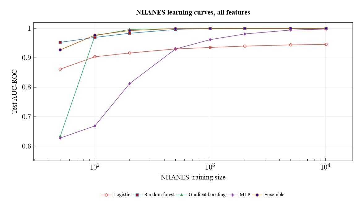
NHANES Feature-Set Sensitivity

Model	All features	No eGFR/ACR	No eGFR/ACR/Cr/BUN
LogReg	0.9457	0.8131	0.6926
RF	1.0000	0.9737	0.9218
HGB	1.0000	0.9751	0.9205
MLP	0.9971	0.9690	0.9155
Ensemble	1.0000	0.9749	0.9216

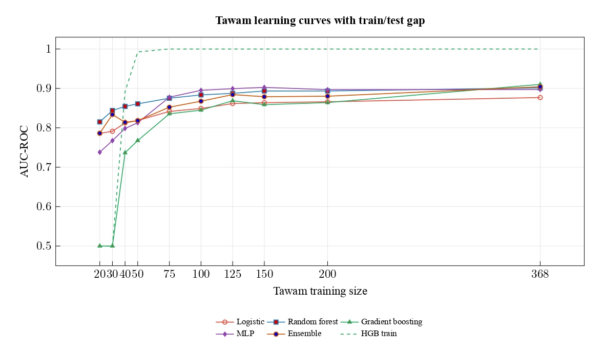
Tawam Learning Curves and Overfitting

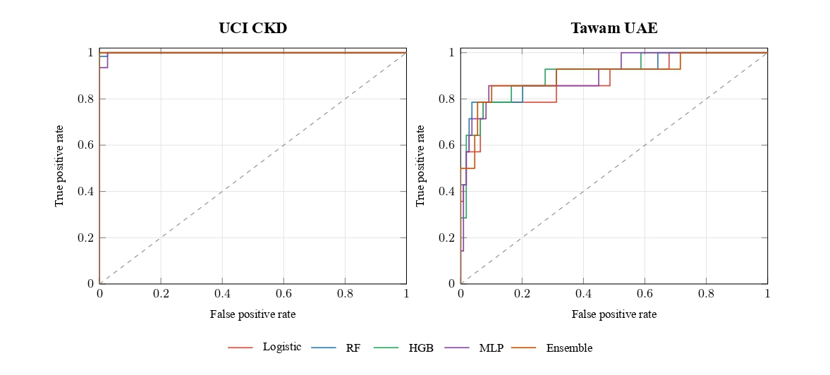
We trained the models on Tawam using baseline measurements to predict which patients developed CKD during follow-up. This means Tawam models more closely predict future outcomes, which differs from UCI, where models mainly identify pre-existing CKD, and NHANES, where CKD is defined based on eGFR and ACR. Models on Tawam produced test AUC values between 0.88 and 0.91 and indicated a 0.03 to 0.10 decrease between training and test AUC values. However, this difference may reflect overfitting but should be interpreted cautiously because only 14 out of the 123 patients in the test group developed CKD, meaning small chance differences in the test group could affect model performance.

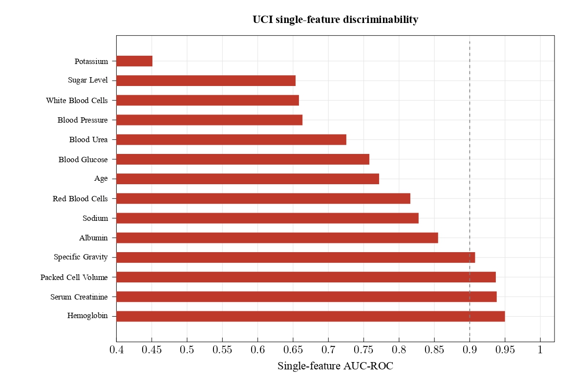
Single-Feature Screening and Ablation

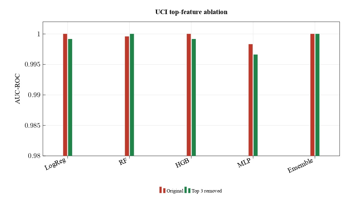
Numerical and ordered UCI predictors were tested individually using logistic regression, with the four strongest measurements being hemoglobin, serum creatinine, packed cell volume, and specific gravity. Each measurement separated the CKD and non-CKD cases well, producing test AUC values between 0.91 and 0.95, medically plausible results consistent with their relationships to CKD. This becomes clearer when we consider what each measurement represents. Serum creatinine helps estimate kidney filtration, urine specific gravity reflects urine concentration, and lower hemoglobin and packed cell volume are both associated with established CKD^2,18. Even though these results may all be plausible, many UCI patients already have relatively advanced disease, which may allow even one laboratory measurement to distinguish between CKD and non-CKD groups unusually well.

Cross-Dataset Transfer

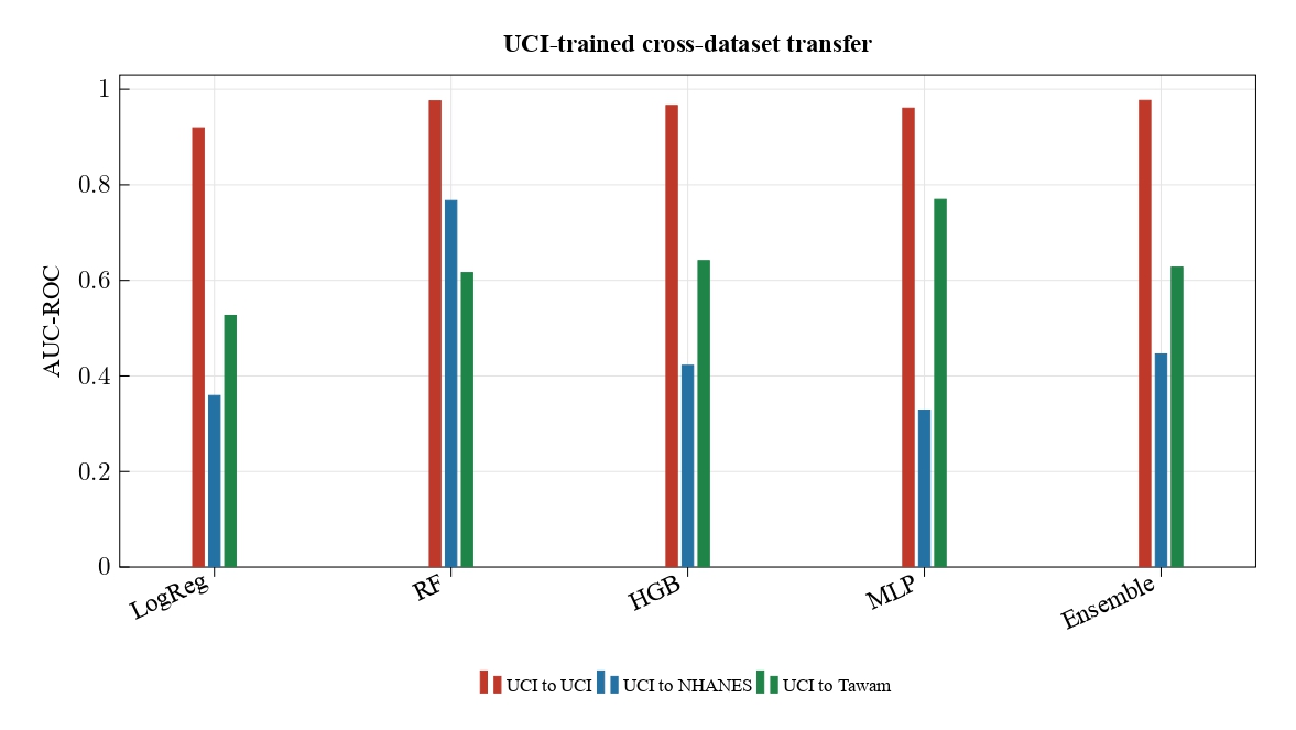
We trained models on UCI using the three shared predictors: age, systolic blood pressure, and serum creatinine. This helped us determine whether the patterns learned from UCI would remain useful in other datasets. When we applied UCI-trained models to NHANES and Tawam without additional training, the AUC values were lower and had more variation across models compared to three-predictor UCI test results. The results suggested that relationships learned from UCI did not transfer consistently across datasets. This finding is similar to other medical-AI studies, which show that models that perform well within their original datasets may perform worse when applied to different patient groups and clinical settings^12,14.

Power-Law Summaries

Model	c ceiling	a	b	R2	Drop–2 c
All features
LogReg	0.946 (0.946–0.953)	1.736 (0.349–3.156)	0.780 (0.427–0.929)	0.990	0.950
RF	1.000 (1.000–1.000)	1.446 (0.889–199.994)	0.864 (0.746–1.774)	0.980	1.000
HGB	1.000 (1.000–1.000)	200.000 (14.296–200.000)	1.637 (1.560–1.965)	0.923	1.000
MLP	1.000 (1.000–1.000)	4.790 (2.996–49.663)	0.629 (0.513–1.053)	0.948	1.000
Ensemble	1.000 (1.000–1.000)	49.917 (45.269–199.971)	1.668 (1.646–1.969)	1.000	1.000
No eGFR/ACR
LogReg	0.813 (0.813–0.814)	12.850 (1.612–22.715)	1.305 (0.869–1.449)	0.996	0.813
RF	0.974 (0.974–0.978)	1.195 (0.402–1.461)	0.731 (0.502–0.782)	0.998	0.977
HGB	0.975 (0.975–0.989)	200.000 (0.383–200.000)	1.636 (0.428–1.642)	0.972	0.981
MLP	1.000 (0.972–1.000)	2.658 (1.571–200.000)	0.448 (0.318–1.211)	0.859	0.973
Ensemble	0.975 (0.975–0.986)	3.498 (0.172–9.804)	0.946 (0.303–1.203)	0.978	0.985
No eGFR/ACR/Cr/BUN
LogReg	0.693 (0.693–0.696)	4.643 (0.772–9.046)	1.038 (0.655–1.204)	0.995	0.694
RF	0.922 (0.921–0.925)	2.417 (0.910–2.573)	0.786 (0.589–0.803)	0.999	0.925
HGB	0.919 (0.919–0.953)	200.000 (0.228–200.000)	1.672 (0.201–1.680)	0.973	0.947
MLP	1.000 (0.918–1.000)	1.782 (1.284–129.410)	0.325 (0.246–1.113)	0.869	0.921
Ensemble	0.921 (0.921–0.938)	5.530 (0.217–17.151)	0.968 (0.276–1.251)	0.975	0.937

Discussion

The UCI Ceiling

We believe that UCI has limited value for measuring CKD ML progress for three reasons. First, all five models produced AUC values concentrated toward 1.0, making differences in performance difficult to distinguish. Second, several models separated CKD and non-CKD groups well, even at small training sample sizes. The models’ performance suggests that the differences were not difficult to learn. Third, complete predictor sets were not needed to achieve high performance, as individual measurements like hemoglobin and serum creatinine already distinguished CKD from non-CKD records when tested alone. Previous research is consistent with this view. Strong scores may not apply beyond the specific patients and tasks studied, and using test data in model preparation may artificially inflate performance to make the model appear better than it is^11,20.

Right Problem, Wrong Population

UCI has limited usefulness as a model-comparison benchmark because all five models achieve similar AUC values. However, UCI still has other use cases. It represents a specific scenario where measurements reflecting CKD are already present, and tests whether the model can distinguish between hospital CKD and non-CKD records. Early screening is more difficult since it tests models’ ability to identify CKD among patients before they show symptoms or pronounced signs of disease. However, the small size of UCI allows for quick training, and it contains missing values and different variables that remain useful for practicing data cleaning and preparation. High model performance on UCI should be treated skeptically; it neither describes the model’s ability to screen new patients nor provides clinical guidance. We could only consider the models clinically useful if the models were tested on independent data that represent both the intended patient population and the intended clinical tasks^12,11

NHANES Circularity

NHANES illustrates a different reason for unusually high AUC values. Participants were classified as having CKD based on their eGFR and ACR values, with those same two measurements also given to the models¹⁸. Since these two measurements are both predictors and the basis for determining CKD status, the models received direct access to the measurements behind the outcome. This also reduced reliance on separate clinical information to identify participants with CKD. When we performed feature removal, the models showed a performance decline when eGFR and ACR were removed. Performance declined even further when we also removed creatinine and BUN. The high results can be explained by two situations. UCI has near-perfect performance because CKD and non-CKD groups already have pronounced differences, while NHANES depends largely on measurements of kidney function and damage.

Ablation Interpretation

The UCI ablation results show that its near-perfect results are not dependent only on the three strongest individual predictors. The three strongest predictors – hemoglobin, serum creatinine, and packed cell volume – performed well when tested alone, but removing all three of these predictors together had little effect on model performance when the models were retrained. The lack of a substantial performance decline suggests that several related UCI measurements provide information about established CKD. This resembles shortcut learning, where models can rely on several related clues that work well within one dataset but fail to remain useful in other settings^13,14. However, even after we removed the three strongest measurements, we cannot show whether any remaining measurement directly reveals CKD or what specific measurements allow model performance to remain high.

Implications

A near-perfect AUC on one small CKD dataset is insufficient to determine whether a certain model outperforms others or performs well in other patient populations. For this reason, CKD models benefit from multiple training/test splits, as evaluating only one provides limited information. Appropriate model checks depend on the intended clinical purpose. These could include testing on independent populations, examining learning curves, screening individual predictors, removing feature sets, examining calibration plots, and measuring performance at clinically relevant decision thresholds^11,14,15,20. The Tawam results demonstrate the importance of these additional evaluations most clearly. Although random forest and the ensemble achieved AUC values around 0.90, their sensitivities at the 0.5 threshold were only 0.143 and 0.286. In the test group, this means that they identified only 2 and 4 of the 14 patients who developed CKD, respectively. This meant that the models could still rank patients well despite missing most CKD cases when using a 0.5 threshold to classify their predictions. Before clinical application, future researchers should select and evaluate the appropriate threshold based on both the intended clinical use and the consequences of false-negative and false-positive results.

Limitations

We used publicly available datasets that were originally created for other purposes. This means that our analysis inherits limitations in the datasets’ patient groups and clinical measurements. For Tawam, the dataset only came from one hospital and only 56 patients developed CKD. The differences in its training/test performance could be interpreted as either overfitting or chance variations in the sample. Since the dataset only came from one center, the performance results could reflect possible instability and should not be considered evidence that similar performance would occur at other centers^16,20. For NHANES, we examined the dataset as a machine learning benchmark instead of its original purpose as a national survey. Because we did not use survey weights and sampling-design variables in our analysis, our analysis does not provide a nationally representative estimate of CKD prevalence in the US population¹⁹. The cross-dataset evaluation was also limited to three variables, limiting how comprehensively the experiment could evaluate UCI-trained model performance on NHANES and Tawam. Along with these dataset-related limitations, the power-law analysis also requires caution. We calculated our estimates from the observed NHANES learning curves, but different models, predictors, or patient samples in other studies could produce different ceiling estimates. Although the power-law equation projects the learning curves beyond the training sizes we used in our analysis, its ceiling does not establish a cap on possible CKD prediction performance. This is especially true when a parameter reaches its maximum allowed value; this means that the fitting procedure reached its boundary, and the result should not be treated as a precise estimate.

Some considerations central to clinical ML were also beyond the scope of our analysis. We did not examine demographic fairness or compare the accuracy of predicted CKD probabilities across patient subgroups, both of which are important considerations in clinical ML²³. Our model comparison was also not exhaustive. We included five models, but we excluded newer tabular foundation models such as TabPFN²⁴. The conclusions in this analysis should also be limited to the datasets and methods studied and should not be assumed to apply to every patient or clinical setting.

Concluding Remarks

UCI should not be discarded, but the results supported more limited applicability. The dataset’s small size remains useful for quickly training models, and it contains missing values and variables suitable for missing-value imputation, conversion of categories into numerical form, and teaching training and test splits. However, UCI could not meaningfully distinguish the five models tested in our analysis and should not be taken as proof of progress in CKD machine learning or of clinical usefulness.

Tasks that included less information or asked for future predictions produced lower AUC values. Their results were more variable than on UCI, had clearer differences between models, and showed more gradual improvements as we increased training data. UCI performance, by comparison, was near perfect, even after removing the three strongest individual predictors. When we used the three shared variables between all three datasets, and applied UCI-trained models to NHANES and Tawam, the resulting AUC values declined and varied more. However, this comparison was not comprehensive, and should be taken cautiously, as there were only three shared variables between the datasets. In order to investigate clinical usefulness, we suggest that future research evaluate models on independent datasets that align with the intended patient populations and clinical tasks.

Data and Code Availability

The analysis code and regenerated output files underlying the tables and figures are available in the GitHub repository (https://github.com/jxia2027-cloud/NHSJS.git). The analysis script is provided as datasetsPythonScripts/nhsjs.py. Regenerated outputs are provided as outputs/results.json and as CSV files in outputs/latex_data/. These files contain only de-identified derived data tables and model-output summaries. The source datasets are publicly available from the UCI Machine Learning Repository, CDC/NCHS NHANES, and the published Tawam cohort cited in this manuscript.

Acknowledgments

The author thanks the UCI Machine Learning Repository, CDC/NCHS for NHANES 2021–2023, Tawam Hospital for the published CKD cohort, and American Heritage School for supporting independent research.

References

1. B. Bikbov, C. A. Purcell, A. S. Levey, et al. Global, regional, and national burden of chronic kidney disease, 1990–2017: a systematic analysis for the Global Burden of Disease Study 2017. Lancet. Vol. 395, No. 10225, pg. 709–733, 2020, DOI: https://doi.org/10.1016/S0140-6736(20)30045-3. [↩]
2. A. S. Levey and J. Coresh. Chronic kidney disease. Lancet. Vol. 379, No. 9811, pg. 165–180, 2012, DOI: https://doi.org/10.1016/S0140-6736(11)60178-5. [↩] [↩] [↩]
3. M. A. Islam, M. Z. H. Majumder, and M. A. Hussein. Chronic kidney disease prediction based on machine learning algorithms. Journal of Pathology Informatics. Vol. 14, article 100189, 2023, DOI: https://doi.org/10.1016/j.jpi.2023.100189. [↩]
4. P. Chittora, S. Chaurasia, P. Chakrabarti, et al. Prediction of chronic kidney disease: a machine learning perspective. IEEE Access. Vol. 9, pg. 17312–17334, 2021, DOI: https://doi.org/10.1109/ACCESS.2021.3053763. [↩] [↩]
5. R. K. Halder, M. N. Uddin, M. A. Uddin, et al. ML-CKDP: machine learning-based chronic kidney disease prediction with smart web application. Journal of Pathology Informatics. Vol. 15, article 100371, 2024, DOI: https://doi.org/10.1016/j.jpi.2024.100371. [↩]
6. E. Dritsas and M. Trigka. Machine learning techniques for chronic kidney disease risk prediction. Big Data and Cognitive Computing. Vol. 6, No. 3, article 98, 2022, DOI: https://doi.org/10.3390/bdcc6030098. [↩]
7. H. Chen, Y. Huang, and L. Chen. Ensemble machine learning for predicting renal function decline in chronic kidney disease: development and external validation. Frontiers in Medicine. Vol. 12, article 1598065, 2025, DOI: https://doi.org/10.3389/fmed.2025.1598065. [↩]
8. L. J. Rubini, P. Soundarapandian, and P. Eswaran. Chronic kidney disease. UCI Machine Learning Repository, 2015, DOI: https://doi.org/10.24432/C5G020. [↩] [↩] [↩]
9. A. Salekin and J. Stankovic. Detection of chronic kidney disease and selecting important predictive attributes. 2016 IEEE International Conference on Healthcare Informatics (ICHI). pg. 262–270, 2016, DOI: https://doi.org/10.1109/ICHI.2016.36. [↩]
10. S. M. Ganie, P. K. Dutta Pramanik, S. Mallik, and Z. Zhao. Chronic kidney disease prediction using boosting techniques based on clinical parameters. PLOS ONE. Vol. 18, No. 12, article e0295234, 2023, DOI: https://doi.org/10.1371/journal.pone.0295234. [↩]
11. G. S. Collins, K. G. M. Moons, P. Dhiman, et al. TRIPOD+AI statement: updated guidance for reporting clinical prediction models that use regression or machine learning methods. BMJ. Vol. 385, article e078378, 2024, DOI: https://doi.org/10.1136/bmj-2023-078378. [↩] [↩] [↩] [↩] [↩]
12. J. R. Zech, M. A. Badgeley, M. Liu, et al. Variable generalization performance of a deep learning model to detect pneumonia in chest radiographs: a cross-sectional study. PLOS Medicine. Vol. 15, No. 11, article e1002683, 2018, DOI: https://doi.org/10.1371/journal.pmed.1002683. [↩] [↩] [↩]
13. R. Geirhos, J. H. Jacobsen, C. Michaelis, et al. Shortcut learning in deep neural networks. Nature Machine Intelligence. Vol. 2, pg. 665–673, 2020, DOI: https://doi.org/10.1038/s42256-020-00257-z. [↩] [↩]
14. C. Ong Ly, B. Unnikrishnan, T. Tadic, et al. Shortcut learning in medical AI hinders generalization: method for estimating AI model generalization without external data. npj Digital Medicine. Vol. 7, article 124, 2024, DOI: https://doi.org/10.1038/s41746-024-01118-4. [↩] [↩] [↩] [↩]
15. B. G. Hill, F. L. Koback, and P. L. Schilling. The risk of shortcutting in deep learning algorithms for medical imaging research. Scientific Reports. Vol. 14, article 29224, 2024, DOI: https://doi.org/10.1038/s41598-024-79838-6. [↩] [↩]
16. S. Al-Shamsi, D. Regmi, and R. D. Govender. Chronic kidney disease in patients at high risk of cardiovascular disease in the United Arab Emirates: a population-based study. PLOS ONE. Vol. 13, No. 6, article e0199920, 2018, DOI: https://doi.org/10.1371/journal.pone.0199920. [↩] [↩] [↩] [↩]
17. Centers for Disease Control and Prevention, National Center for Health Statistics. NHANES August 2021–August 2023 questionnaires, datasets, and related documentation. 2024, URL: https://wwwn.cdc.gov/nchs/nhanes/continuousnhanes/default.aspx?Cycle=2021-2023. [↩] [↩]
18. KDIGO CKD Work Group. KDIGO 2024 clinical practice guideline for the evaluation and management of chronic kidney disease. Kidney International. Vol. 105, No. 4S, pg. S117–S314, 2024, DOI: https://doi.org/10.1016/j.kint.2023.10.018. [↩] [↩] [↩] [↩]
19. Centers for Disease Control and Prevention, National Center for Health Statistics. Brief overview of sample design, nonresponse bias assessment, and analytic guidelines for NHANES August 2021–August 2023. 2024, URL: https://wwwn.cdc.gov/nchs/NHANES/continuousnhanes/overviewbrief.aspx?cycle=2021-2023. [↩] [↩]
20. A. Vabalas, E. Gowen, E. Poliakoff, and A. J. Casson. Machine learning algorithm validation with a limited sample size. PLOS ONE. Vol. 14, No. 11, article e0224365, 2019, DOI: https://doi.org/10.1371/journal.pone.0224365. [↩] [↩] [↩] [↩]
21. A. Dayimu, N. Simidjievski, N. Demiris, and J. Abraham. Sample size determination for prediction models via learning-type curves. Statistics in Medicine. Vol. 43, No. 16, pg. 3062–3072, 2024, DOI: https://doi.org/10.1002/sim.10121. [↩]
22. C. Meek, B. Thiesson, and D. Heckerman. The learning-curve sampling method applied to model-based clustering. Journal of Machine Learning Research. Vol. 2, pg. 397–418, 2002. [↩]
23. J. Yang, A. A. S. Soltan, D. W. Eyre, and D. A. Clifton. Algorithmic fairness and bias mitigation for clinical machine learning with deep reinforcement learning. Nature Machine Intelligence. Vol. 5, No. 8, pg. 884–894, 2023, DOI: https://doi.org/10.1038/s42256-023-00697-3. [↩]
24. N. Hollmann, S. Muller, L. Purucker, et al. Accurate predictions on small data with a tabular foundation model. Nature. Vol. 637, pg. 319–326, 2025, DOI: https://doi.org/10.1038/s41586-024-08328-6. [↩]