Sea Level Rise Prediction in Miami Beach using Continuous Time Markov Chains, Random Forest Regressions, and Seasonal ARIMA Models

Abstract

Rapid sea level rise poses immediate risks to coastal cities, like Miami Beach, with accurate forecasting technologies having the potential to inform infrastructure and adaptation. This study evaluates probabilistic state-transition models (Continuous-Time Markov Chains) and compares its effectiveness and accuracy to Random Forest (RF) Regressions and Seasonal ARIMA (SARIMA) models using identical datasets and evaluation windows. Monthly Mean sea level data of Miami beach from PSMSL Revised Local Reference (RLR) tide-gauge record was used to train the models, with data ranging from June 1931 to May 1981. Firstly, CTMC discretized data into 6 fixed state bins by rounding values to the nearest 100mm, and then estimated transition counts to project future state distributions and sea level rise. RF integrated temporal features (lagged sea-level values, month-of-year indicators) and SARIMA used a seasonal structure fitted for monthly geophysical data; both were evaluated on the same chronological train/test splits. Performance was assessed using R², RMSE, and MAE: RF performed best (R²=0.515; RMSE=55.61 mm; MAE=43.66 mm), followed by SARIMA (R²=0.468), and lastly CTMC (R²≈−0.044). The 24-month forecasts (RLR units; subtract 7000 mm to obtain raw sea level) were 7000.42 mm (CTMC), 7020.07 mm (RF), and 7128.07 mm (SARIMA). CTMC, though underperforming in modeling the nonlinear dynamics of sea level, showed great framework interpretability, motivating future research for richer state definitions and additional covariates (tides, storm surges, CO₂). 

Keywords: Miami Beach, Sea Level Rise, Continuous-Time Markov Chains, Random Forest, SARIMA, Time-Series Forecasting

Introduction

As climate change becomes a widespread crisis, global warming and the changing of environments and ecosystems become seemingly more impactful, with sea levels rapidly rising across the world. For example, over the course of the past 244 years, specifically since 1880, the global mean sea level has risen approximately 8-9 inches¹. Some of the causes attributed to this crisis include the combination of melting water from glaciers and ice sheets, as well as the expansion of warming sea water, which all stems from global warming. Furthermore, in the United States, over 30% of the population live in coastal areas¹, where sea level influences coastal flooding, erosion, storm hazard, and more. Additionally, along coastal cities, sea level rise threatens infrastructure as a whole, thereby contributing and affecting jobs. Serving as a prime example, Miami Beach is one of the major cities in the United States at severe risk of rising sea levels, with some regional projections estimating approximately 14 to 26 inches of sea level rise in Southeast Florida by 2060². This places low-lying areas of Miami-Dade County at significant risk. Therefore, it is imperative to be able to model and predict sea levels in order to make efforts to reduce its devastating impacts as well as take preemptive actions against it.

The study implemented CTMC as an interpretable, discretized baseline rather than a calibrated climate projection. It served as a finite-state homogeneous chain with constant rates converging to a stationary distribution and cannot, by construction, reproduce an externally forced upward trend, so it is included for mechanistic comparisons against the RF and SARIMA models. To address this world crisis, this study introduces a novel approach utilizing mathematical models such as the Continuous Time Markov Chain (CTMC), trained on decades of data based on sea level rise (meters) in Miami Beach. A CTMC is a stochastic continuous model that allows for the prediction of a future state (state j), based on the probabilities of the current or past states (state i) over given amounts of time. It correlates to matrices and can often be described by the transition matrix, which is defined by the term: P_ij, which represents the probability of transitioning from State i to State j. This probability is found by calculating the total transitions from State i to State j over the total transitions in the given State i. The Continuous Time Markov Chain also requires transition rates found within the Q Matrix, which could be calculated by the transition matrix found in the study. Through the division of P_ij and total time spent (in months) in State i, the study discovered the rate of transition per month of sea levels across the defined and categorized states. The fundamental transition prediction probabilities that provide the model with the capabilities to find sea level in the future are calculated by several formulas that involve the initial state distributions as well as P(t) = e^Qt, where Q is the infinitesimal matrix (Q matrix)  and t is the time in between two states. These formulas allow the CTMC to project future state probabilities and corresponding sea-level values for Miami Beach, which this study evaluates against the observed record.

Furthermore, as Continuous Time Markov Chains historically have not been utilized as frequently as various other models to predict sea level rise, it is imperative for the study to determine whether CTMC is appropriate in comparison to other models for such a task. Therefore, the study constructed two machine learning based models, specifically Random Forest and ARIMA based models, trained on the exact same dataset with consistent intervals across the training time period. Random Forests (RF) are ensemble learners that combine multiple decision trees trained on perturbed versions of data whose data points and features have been randomly selected (random feature subspace selection³). Such machine learning and deep learning approaches have recently been applied to tide gauge sea level forecasting in several coastal regions^4,5,6. Random Forest and related ensemble methods, in particular, have been used to forecast tide levels and extend sea-level records^7,8, whereas neural-network models such as NARX have been applied to tide prediction from gauge data

The primary objective of this study is to develop and validate a robust stochastic continuous time markov chain for predicting sea level rise, in meters, specifically in Miami Beach, Florida, and to determine if it serves as an appropriate prediction model in relation to Random Forest and ARIMA for forecasting sea level rise. Through the use of datasets, dating back decades, specifically from 1931, this model is capable of predicting sea level rise per month and sea level at a given moment in time, therefore representing and showcasing a significant enhancement and step to understanding and battling sea level rise under climate change. However, it is imperative to note that this study focuses on monthly mean sea level specifically at Miami Beach; therefore, results may not generalize to other coastlines or to changed windows/periods.

Methods

Continuous Time Markov Chain

A traditional discrete Markov Time Chain remains in one given state for a unit of time before transitioning to another state⁹. However, in hopes of modeling sea level rise where transitions and time spent per transition fail to remain consistent, a discrete Markov Time Chain, {X(n) : n ≥ 0}, is not a suitable stochastic model for modeling a continuous scenario⁹. Therefore, this study employs the use of a Continuous Time Markov Chain which allows a continuous amount of time in any state, therefore randomizing the number of transitions and the probabilities as well, whilst retaining the Markov Property¹⁰. However, this does introduce certain difficulties as there is no set time between each transition but rather an infinite amount of possible continuous times, leading to individual probability calculations from one state to another.

A CTMC requires categorized and distinct states (e.g. S = {s₁,s₂,…,s₆}), in order to find the probabilities between them.  Therefore, this study incorporated 6 states that were categorized by meters in sea level, including 6800mm (state 1), 6900mm (state 2), 7000mm (state 3), 7100mm (state 4), 7200mm (state 5), and 7300mm (state 6).

Upon defining the states of the study, a CTMC can be defined by a Transition Probability Matrix (P), Pij, as it is based on the probabilities of transitioning from one state to another over the total transitions in that given state. Upon finding the probabilities of transitioning from state i to state j, the study discovered the model’s Q matrix, through dividing Pij over the total time spent (in months) in the given states, thereby giving the rate (months) at which sea level transitions through states. The fundamental transition prediction probabilities are calculated by the formula, P(t) = e^Qt, where Q is the infinitesimal matrix (Q matrix) and t is the time in between two states. P(t) provides the study with the exponential matrix, but the function, serves as the final formula that represents sea level after t months. These formulas allow the CTMC to project future state probabilities and corresponding sea-level values for Miami Beach, which this study evaluates against the observed record.

Data Collection

This study utilized a comprehensive dataset consisting of 601 data points to analyze and convert to a Continuous Time Markov Chain. The data was sourced from the National Oceanography Centre (NOC) Permanent Service for Mean Sea Level (PSMSL¹¹), which is a widely reputable and credible source that has been responsible for the monitoring, analysis, collection, and publication of mean sea level data from the global network of tide gauges since the year 1933. Among the 601 data points, 41 data points were invalidated and corrupted, leaving the study with a total of 560 data points. Due to the fact that these corrupted months were removed rather than interpolated, a few consecutive observations are separated by more than one month. However, the model treats every step from one row to the next as a single one-month transition. Where such gaps occur, the true elapsed time is compressed into one step, thereby leading to certain bias in the estimated transition rates. It can be seen that if actual dated spacing was utilized between observations, this limitation would be addressed.

The database was filtered by Station Name and ID, each respectively representing the dataset (mean sea level) of an area or city within the world. This study analyzed the dataset pertaining to Miami Beach (Miami Beach Station, ID: 363).

Additionally, it is extremely important to understand that the RLR data provided in the Miami Beach Station are demonstrated to be approximately 7000mm below mean sea level, which PSMSL did in hopes of avoiding negative numbers¹¹. Therefore, the raw sea level numbers provided within the dataset are relative values that are shifted upward by 7000mm to avoid negative numbers in regard to mean sea level values within the dataset. Therefore, all expected and predicted values should be easily adjusted by subtracting 7000mm to determine the real-world interpretable results in relation to actual sea level rise.

Data Utilization/Preparation

The variable that was modeled within the CTMC was sea level rise in millimeters (mm). However, within CTMC, states must be accessible and have the ability to transition from one another, such that both states communicate⁹. Furthermore, as the CTMC Model is traditionally used to analyze distinct categorical variables (states) in order to record and calculate transitions and rates between them, this study, accordingly, categorized sea level rise (mm), in regards to being shifted by 7000mm, into 6 discrete states: 6800 mm (State 1), 6900 mm (State 2), 7000 mm (State 3), 7100 mm (State 4), 7200 mm (State 5), and 7300 mm (State 6).

The data points were then filtered into each of the states/categories by rounding to the nearest hundred (e.g. 7190 mm was placed in the 7200 mm category, 6946 mm was placed in the 6900 mm category). Upon completing the systematic and through filtering process, the distribution of data points in the states was as followed: State 1 (6800 mm) contained 6 data points, State 2 (6900 mm) contained 147, State 3 (7000 mm) contained 234, State 4 (7100 mm) contained 116, State 5 (7200 mm) contained 48, and State 6 (7300 mm) contained 9. States 1 and 6 are represented by only 6 and 9 of the 560 observations, so transition probabilities and rates involving these states are estimated from very few events and should be treated as highly uncertain.

However, it is important to highlight that the rounding of data points by the nearest hundred can contribute to a loss of accuracy and precision, leading to faulty insights. Nevertheless, it was necessary as it reduces variability and improves generalization when categorizing and analyzing in time series format for the Continuous Time Markov Chain.

As CTMC revolves around probabilities of transitioning from state i to state j, the study moved forward to analyze and count the transitions from one state to another across the 560 data points. Assuming t, represents the date of a single row, the study noted whenever a change of state occurred between t and t + 1, or simply, whenever a transition occurred between two different states (e.g. 6800 mm and 7200 mm) across rows. Therefore, for each state, the number of transitions to all other states, including self-transitions, was systematically counted (e.g. number of transitions from state 1 to states 1–6, from state 2 to states 1–6, and so on through state 6 (including). It was found that there were a total of 6 transitions from and in State 1, 147 transitions for State 2, 232 transitions for State 3, 111 transitions for State 4, 48 transitions for State 5, and 9 transitions for State 6. It is found that the number of transitions is not equivalent to the number of data points, thereby raising concerns over accuracy or miscounting, however, this result stems from the lack of transitions to the data points which were corrupted or invalidated, leading to some data not transitioning properly and hence being skipped.

	6800s (State 1)	6900s (State 2)	7000s (State 3)	7100s (State 4)	7200s (State 5)	7300s (State 6)
6800s (S1)	1	4	1	0	0	0
6900s (S2)	3	81	57	6	0	0
7000s (S3)	1	52	123	45	11	0
7100s (S4)	0	4	41	39	23	4
7200s (S5)	1	0	12	20	10	5
7300s (S6)	0	0	0	5	4	0

Transition Matrix P

The Transition Matrix P, is often defined by P_ij, which determines the probability of transitioning from State i to State j. This probability is calculated through the formula:

Equation 1: Transition Matrix P

The study constructed a six by six transition matrix by dividing the individual and respective transitions of each state and dividing by the total transitions within that state. This methodology and systematic procedure was conducted for all 36 possibilities for the six states within the six by six matrix, where each row summed to 1. For example, to calculate P₁₃, which refers to the probability of transitioning from State 1 to State 3 and is calculated by taking the number of transitions from State 1 to 3, which is 1, and dividing by the total transitions within State 1: 6. Therefore, the transitional probability would be ⅙ or 0.1666667.

Infinitesimal Generator Matrix Q

The Infinitesimal Generator Matrix (Q Matrix), is defined by Q_ij, and calculates a similar probability to the prior probabilities calculated for the transition matrix, however it refers to the rate of change and the instantaneous probability/transition rate of transitioning from State i to State j per unit of time. In regards to this study, it calculated the rate at which the variable, Sea Level Rise (mm), changed in states per month (unit of time). The formula used to calculate Q_ij is as follows:

The Q matrix and its transition rates are found by dividing P_ij, where P_ij (probability within the Transition Matrix) is the probability of transitioning from State i to State j, and T_i, where T_i, is the total time spent in months in State i. A six by six Q Matrix was constructed, calculating the rate of change of transitional probabilities for each of the six states. For instance, Q₃₂, which refers to the Q probability from State 3 to State 2, is calculated by dividing P₃₂ (0.2241379) and T₃ (232), which gives you a Q transition rate of 0.000958.

Additionally, it is imperative to note the significant difference between the Q Matrix and P Matrix where the diagonal elements of the Q matrix must be negative and rows must sum to 0. Therefore, the elements Q₁₁, Q₂₂, Q₃₃, Q₄₄, Q₅₅, Q₆₆ all must be negative. This ensures that the total rate out of a state is equal to the sum of the rates in respect to the other states, thereby reflecting the memoryless property of CTMCs and leading to the total rate of departure being accurate. In other words, for each row i, the diagonal entry satisfies Q_ii = −Σ_j≠i Q_ij, so that the entries in each row of Q sum to zero. Equation 3: Infinitesimal Generator Matrix Q per Row

Prediction Formulas

Though the transitional probabilities in relation to time have been calculated, the continuous time markov chain must predict sea level rise in the future, thereby outputting relevant numbers and units in respect to sea level and the time in months. As this study’s purpose is to predict future sea level, not just calculate state probabilities, ) must be calculated for it also represents the row vector that provides the probability of being in each state after t units of time (months). The study used the CTMC prediction formula:

Equation 4: Initial State Probabilities

Upon systematically inputting and calculating the variables variables (e.g. e^Qt and , ) was successfully was successfully found, consequently providing future sea level values in regards to the dataset. Once ) was calculated, the formula:

Equation 5: Sea Level Rise Prediction

Where ) is the state-probability row vector and Sᵀ the sea-level value assigned to each state (6800–7300 mm).

Random Forest Regression (RF) Construction

This study also constructed an in-depth Random Forest machine learning based model, employing the RF regressor to keep a non-parametric machine learning benchmark, and implementing the model in Google Colab in Python using scikit-learn (from sklearn.ensemble import RandomForestRegressor) along with NumPy and pandas for data handling (import numpy as np, import pandas as pd). Performance metrics were then computed with r2_score, mean_squared_error, and mean_absolute_error from sklearn.metrics.

Similar to CTMC, the study transformed the identical dataset and values of monthly sea level record in Miami Beach into a supervised-learning dataset, a requirement for RF. Using custom functions such as numpy slicing, the input-target pairs were constructed (X_t, y_t) with each feature vector X_t consisting of the previous 24 months of sea level along with several engineered predictors. The target feature y_t was the sea level 24 months ahead. Lastly, for each time index t, it included the 24 raw lag values (s_t-24,…,s_t-1​), the month-of-year for the specific prediction time, where in this study was t+24 (months from pandas.DatetimeIndex.month), and a 12-month rolling mean computing the Numpy over s_t-12,…,s_t-1.

This produced a design matrix of shape (509, 27) and a finalized target vector of length 509.

Furthermore, the data was then split chronologically using simple custom splits, where the first 80% of the data was used as training, and the last 20% were used for testing/backtesting, thereby yielding the Random Forest Model in this study 407 training samples, and 102 test samples. This respected time ordering, avoided leakage, and minimized overfitting.

To fully train the model and test, the study instantiated with the RandomForestRegressor class from scikit-learn with various set parameters to maximize efficiency:

The Random Forest regressor was configured with n_estimators = 300 (the number of decision trees), max_depth = None (no depth limit), min_samples_leaf = 2 (each leaf containing at least two samples), max_features = “sqrt” (a square-root feature subset at each split), random_state = 42 (a fixed seed for reproducibility), and n_jobs = −1 (parallel computation).

The Random Forest was then fit and trained using rf.fit (X_train, y_train). Lastly, the study incorporated an innovative approach to improve correlation and maximize predictive capability by utilizing GridSearchCV with TimeSeriesSplit (from sklearn.model_selection import TimeSeriesSplit, GridSearchCV), a machine learned technique that evaluates every possible combination of hyperparameters to find the most optimal setting for the model¹².

Seasonal ARIMA (SARIMA) Construction

Finally, to complement the machine-learning approach for comparison, the study constructed a classical statistical time-series model, specifically a Seasonal Autoregressive Integrated Moving Average Model (SARIMA). As mentioned, ARIMA models forecast time series by combining the autoregressive (AR), differencing (I), and moving-average (MA) components, thereby providing the ability to capture persistence, shocks, and stochastic variations within the dataset. However, because sea level exhibits an annual seasonal cycle, the study decided to extend the classical ARIMA framework with a seasonal AR and MA term at a 12-month period, resulting in a SARIMA model structure suited for monthly geophysical data¹³. The SARIMA model was constructed in Google Colab using the SARIMAX class from the statsmodel library. As done with the RF and CTMC, the complete monthly sea-level dataset, including 557 viable observations/entries from June 1931 to May 1981) was split chronologically into a training window of 407 months and a test window of 150 months using pandas.read_excel. This matched the time horizon and window split used in all other models, hence allowing for a generalizable and appropriate comparison. The structure utilized for the SARIMA model:

Additional packages and libraries such as numpy, pandas, sklearn.metrics were used for data processing, evaluation, and metric computation (R^2, RMSE, MAE).

For the fitting and model specification, through exploratory tests it was determined that a model with first differencing and single-order seasonal structure captured both the long-term trend and annual oscillations. Therefore, the SARIMA model was specified with the following parameters and values:  Candidate orders were compared by Based on the AIC and BIC values reported in Fig. 1, the selected SARIMA specification (1, 1, 1)(1, 0, 1)12 produced the best out-of-sample test performance, with an R² value of 0.468. In contrast, lower-AIC alternatives, such as the seasonally differenced (1, 1, 1)(1, 1, 1)₁₂ model, performed worse on the held-out
window, with an R² value of 0.416.

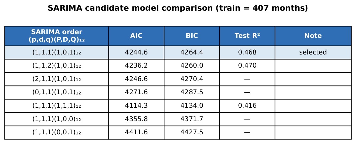
Note: the selected order gives the best out-of-sample test R² even though a seasonally differenced model has lower AIC, supporting the choice on forecast skill.

Furthermore, the SARIMA model used a non-seasonal order of (1,1,1) along AR(1), first differencing, and MA(1), with a seasonal order of (1,0,1,12) capturing annual structure, and was fit with enforce_stationarity = False and enforce_invertibility = False to avoid forced reparameterization.

Finally, one-step-ahead predictions and multi-step forecasts were then obtained through the command lines: fit.predict() and fit.get_forecast(). The sea level rise forecast 24 months ahead (2 years) was then finalized and generated by re-fitting the SARIMA model on the completed 557-month record, with the forecast being run using:

Fit_full.get_forecast(steps=24).predicted_mean

This outputted the model’s prediction for 2 years after the end of the dataset, allowing an unbiased and direct comparison with the Random Forest and CTMC forecasts.

Ethical Considerations: Not applicable as this study does not involve human or animal participants, with data stemming from publicly available tide-gauge repositories.

Results

State Categorization Results

Table 2 summarizes the distribution of the 560 valid observations across the six sea-level states and the resulting initial state probabilities.

Category (mm)	Amount in Category	Total Data Points (n)	State probabilities
6800 (State 1)	6	560	0.0107
6900 (State 2)	147	560	0.2625
7000 (State 3)	234	560	0.4179
7100 (State 4)	116	560	0.2071
7200 (State 5)	48	560	0.08571
7300 (State 6)	9	560	0.01607 State 3 held the highest proportion of observations (41.79%), while the tail states (1 and 6) each held under 2%, indicating sea level was predominantly concentrated in mid-range states throughout the study period.

Transition Matrix

Table 3 presents the six-by-six transition matrix constructed from the state counts in Table 1, with each row summing to 100%.

Probability	6800s (State 1)	6900s (State 2)	7000s (State 3)	7100s (State 4)	7200s (State 5)	7300s (State 6)
6800s (S1)	16.6667%	66.6667%	16.6667%	0.0000%	0.0000%	0.0000%
6900s (S2)	2.0408%	55.1020%	38.7755%	4.0816%	0.0000%	0.0000%
7000s (S3)	0.431034%	22.41379%	53.01724%	19.3966%	4.7414%	0.0000%
7100s (S4)	0.0000%	3.6036%	36.9369%	35.1351%	20.7207%	3.6036%
7200s (S5)	2.0833%	0.0000%	25.0000%	41.6667%	20.8333%	10.4167%
7300s (S6)	0.0000%	0.0000%	0.0000%	55.5556%	44.4444%	0.0000%

Note: The matrix is provided in table format to enhance clarity and readability

Several transitions carry a probability of 0 (e.g. State 4→1, States 1→4/5/6), confirming that distant-state jumps did not occur. The highest observed probability was State 1→2 (≦66.67%), while the lowest non-zero was State 3→1 (0.43%).

Infinitesimal Generator (Q) Matrix

The Infinitesimal Generator Q Matrix provided the study and the CTMC the rate at which state i transitioned to state j per unit of time (months). By utilizing the probabilities calculated from the transition matrix (P_ij) and dividing such by the total time spent in State i, the six by six Q Matrix was constructed, where all diagonal elements remained negative and all rows summed to 0 in order to gain accurate total rates of departure and follow the CTMC properties/requirements.

From \ To	6800s (State 1)	6900s (State 2)	7000s (State 3)	7100s (State 4)	7200s (State 5)	7300s (State 6)
State 1	-0.1389	0.1111	0.0278	0.0000	0.0000	0.0000
State 2	0.0001	-0.0031	0.0026	0.0003	0.0000	0.0000
State 3	0.0000	0.0010	-0.0020	0.0008	0.0002	0.0000
State 4	0.0000	0.0003	0.0032	-0.0056	0.0018	0.0003
State 5	0.0004	0.0000	0.0052	0.0087	-0.0165	0.0022
State 6	0.0000	0.0000	0.0000	0.0617	0.0494	-0.1111

Note: The matrix is provided in table format to enhance clarity and readability. Values < 0.00005 shown as 0.0000 due to rounding.

Equation 2: Infinitesimal Generator Matrix Q

the study successfully found the transition rate probabilities; the highest off-diagonal rate, _Q12 = 0.1111, represents State 1→State 2 (estimated from only six observations and therefore highly uncertain).

Markov Chain Transition Visualizations

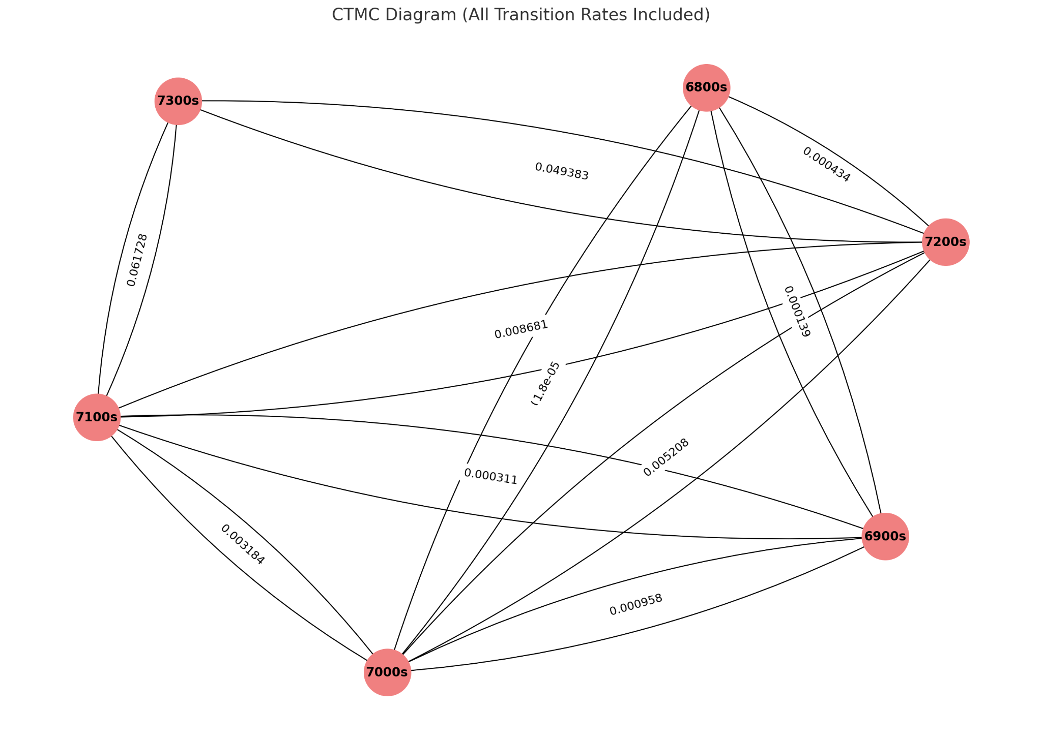
Fig 2 serves as a visual representation of the Continuous Time Markov Chain model using a transition diagram that summarizes the key transition rates between all six states effectively and accurately (e.g. 6800, 6900, and so on). Each node refers to and defines a sea level range (State), with the directed edges/lines representing the transition rates per month (unit of time) of Sea Level Rise between all respective states (Q_ij), which were derived from the calculated Infinitesimal Generator Q Matrix. Transitions predominantly connect adjacent states (e.g. Q₂₃ = 0.0026, Q₃₂ = 0.0010), consistent with incremental monthly sea-level change; the highest off-diagonal rate Q₁₂ = 0.111 is estimated from only six State 1 observations and carries high uncertainty.

Predictive Model Output/Final Results

It is important to note that the sea level values within this study are based on the Revised Local Reference (RLR) database¹¹, which defines its zero datum to be approximately 7000mm below mean sea level. This offset was used to avoid negative numbers when providing mean sea level and annual sea level. Therefore, all predicted values, such as 7010.69 mm and 7000.42 mm, are relative to the RLR baseline. This in turn would lead the interpretation of these values to be 10.69 mm above mean sea level and 0.42 mm above mean sea level, not 7010.69 mm over mean sea level or 7000.42 above mean sea level within Miami Beach. This interpretation and formatting does not affect the accuracy and or structure of the CTMC model, but is important to understand when applying and interpreting the predicted magnitudes of the sea level rise within Miami Beach.

As mentioned, the formula used to predict sea level rise in the future with respect to time for the Continuous Time Markov Chain were the following:

Equation 4: Initial State Vector Probabilities

Where is the initial state vector, eᴸᵗ the matrix exponential over t months, and )the resulting state-probability distribution.

Equation 5: Sea Level Rise Prediction

The study found the initial state/vector distribution , the probability distribution across all states at the starting time (e.g. t = 0 months), by dividing the time spent in State i (months) by the total time in total. Providing the dataset in the format of  = [S1, S2, S3, S4, S5, S6], the initial state vector:

= [0.0107, 0.2625, 0.4179, 0.2071, 0.0857, 0.0161]

To forecast the distribution of sea level states after a given time (t, in months), the matrix exponential was calculated, where Q is the infinitesimal transition matrix and t is the time in months.

Equation 6: Matrix Exponential

Due to the complexity of computing higher matrix powers as a result of such a large dataset that was utilized by this study, the series was truncated once convergence was observed, leading to the study numerically converting the exponential matrix using the standardized code from the Python’s scipy.linalg.expm() function. To demonstrate the results as an example within this paper, the study will assume t as 24 months (2 years) and provide the results of the matrix exponential when t = 24. The probabilities found:

States	6800s	6900s	7000s	7100s	7200s	7300s
6800s	0.0364	0.7354	0.2210	0.0065	0.0008	2.00E-05
6900s	0.0009	0.9318	0.0604	0.0066	0.0003	1.00E-05
7000s	0.0002	0.0220	0.9547	0.0188	0.0043	9.00E-05
7100s	9.00E-05	0.0077	0.0726	0.8816	0.0352	0.0029
7200s	0.0023	0.0069	0.1099	0.1783	0.6882	0.0144
7300s	0.0010	0.0045	0.0592	0.5268	0.3323	0.0762

Note: The matrix is provided in table format to enhance clarity and readability

Though the matrix exponential P(t) = e^Qt above was calculated through the use of the Python scipy.linalg.expm function for t = 24, thereby yielding the probability transition matrix based on the instantaneous rates found in the Q Matrix over a 2-year time period, e^Qt is defined numerically by the infinite series expansion:

Equation 7: Q Matrix

Where each term represents increasing powers of the Q Matrix scaled by time.

Upon calculating the matrix exponential states and probabilities as well as the initial state vector, ) was calculated by multiplying the 1×6 row vector by the 6×6 matrix e^Qt, which provides the format: = [p₁(t), p₂(t), p₃(t), p₄(t), p₅(t), p₆(t)]. Therefore, when predicting sea level rise when t = 24 (in 2 years):

(24)= [0.00092, 0.26392, 0.44258, 0.21598, 0.07350, 0.00309]

The study calculated the result through the use of scipy.linalg.expm function and numpy libraries.

These results demonstrate the probability of being in each state after 24 months (2 years). It can be seen that State 3 has the highest probability at 44.258%, whereas States 1 and 6, which can be considered as the extreme tails, only have probabilities of 0.092% and 0.309% respectively.

The final step in order to accurately predict sea level rise (SeaLevel(t) in the correct units (mm) with respect to time, would be to multiply the probabilities calculated ) by the Sea Level assigned to each state (S). The study calculated the dot product of

Therefore, the Continuous Time Markov Chain successfully predicted an expected sea level of approximately 10.69 (7010.69) mm after 2 years (24 months). It can be seen that this value is slightly below the most recent observations, thereby reflecting the model’s convergence toward its stationary distribution rather than a sustained upward trend. As such, with fixed transition rates the CTMC cannot represent the ongoing climate-driven rise.

However, this prediction is 24 months from the baseline distribution of that yields the expected sea level of 7010.69 mm. When the chain is propagated two years forward from its long-run distribution, the expected level is 7000.42 mm, which corresponds to a decrease of 79.58 mm relative to the last observed value (7080 mm in May 1981).

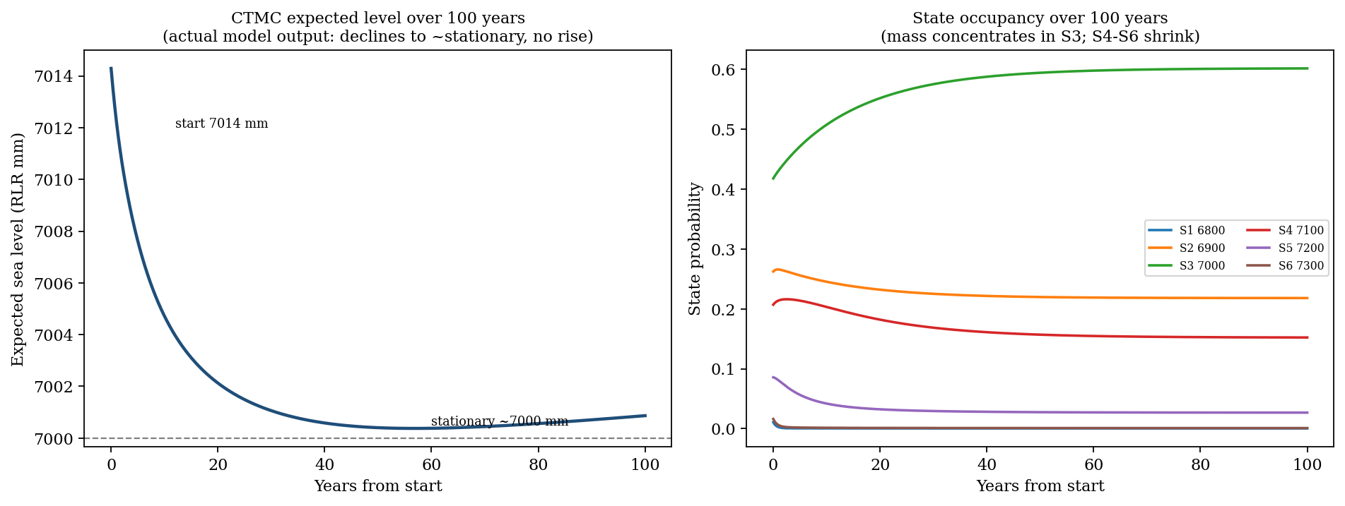
Note: This is not a calibrated sea-level projection; with a constant Q the chain converges to a stationary distribution and the expected level flattens near 7000 mm rather than rising. Predicted Sea Level values in mm are relative to the RLR data baseline (7000 mm below mean sea level)

Fig. 3 shows the CTMC’s expected sea level over the next 100 years under fixed 1931-1981 transition rates. Rather than rising, the expected level drifts downward from approximately 7014 mm and flattens near the baseline of 7000 mm as the chain converges to its stationary distribution. However, because CTMCs have a fixed rate matrix, the predictions and values converge to a stationary distribution and do not entirely reflect the magnitude of the ongoing climate-driven upward trend, therefore highlighting a structural limitation of CTMC compared to RF and SARIMA. This forward curve therefore illustrates the model’s internal structure under fixed rates, rather than a true and accurate forecast of future sea level.

Random Forest Predictive Model Final Results/Output

The Random Forest model produced relative strong predictive performance on the 24-month or 2 year forecasting of sea level rise in Miami Beach. As mentioned prior, by testing the model on the final 102 samples of the dataset and training it on the first 407 samples, the default Random Forest model achieved an R²of 0.515, substantially outperforming the naive last-value baseline which achieved an R² of -0.296. The model had an RMSE of 55.61 mm and an MAE of 43.66 mm, therefore illustrating improved short-term and long-term accuracy relative to the simpler regression strategies. The model when using grid-search hyperparameter tuning actually performed worse on the held-out test window achieving an R² of 0.406, which is lower than the default RF model. Because the series is short and the test set small, the metrics were also checked for stability: across fifteen random seeds the RF test R² was 0.520 ± 0.006 (ranging from 0.510 to 0.530), indicating that the result is not sensitive to the choice of random seed. The lower correlation of the tuned RF is likely attributed to overfitting on the training folds.

The default RF model, which produced the highest correlation(R² = 0.515) predicted a sea level of 7020.07 mm two years into the future from the final data point (May 1981), corresponding to a projected two-year decrease of 59.93 mm from the last observed value in the dataset (7080 mm).

In the model, among the engineered features, the month-of-year indicator was by far the strongest predictor (feature importance approximately 0.48), which allowed the study to confirm a dominant annual cycle. Among the lag features, the 12- and 24-month lags were most informative (approximately 0.09 and 0.05), and a time-index feature contributed approximately 0.07. These importances are summarized in Fig. 4., consistent with feature-importance analyses reported for machine learning sea level models¹⁴

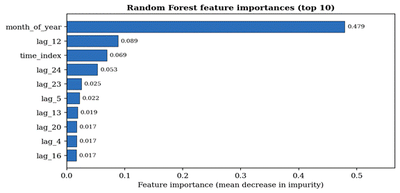
 Note: the month-of-year indicator dominates (approximately 0.48), confirming a strong annual cycle, with the 12- and 24-month lags the most informative lag features.

SARIMA Predictive Model Final Results/Output

The SARIMA model in structure format of (1,1,1)x(1,0,1)₁₂ showed moderate to decent performance relative to the Random Forest when predicting sea level rise in Miami Beach. The performance was consistent with the expectations of the study as it is for linear time-series methods that were applied to a nonlinear geophysical signal. By utilizing the same chronological split between training and testing data points within the dataset, the SARIMA model achieved an R² of 0.468, an RMSE of 60.92 mm, and a MAE of 48.18 mm.

Similar to the Random Forest, the SARIMA model was re-fit on the full 557 month dataset to generate the 2 year prediction from the last data value in the series. The SARIMA prediction produced a sea level of 7128.07 mm for the 2 year forecast that is essentially May 1983. This demonstrated a 48.07 mm increase relative to the last recorded value of 7080 mm in May 1981. Contrasting from the Random Forest, the SARIMA demonstrated a clear increase in sea level rise whereas Random Forest predicted a decline, therefore illustrating the sensitivity of linear statistical models to long-term differencing and seasonal structure.

Comparison of CTMC, RF, and SARIMA

In direct comparison between the three models and forecasting approaches for predictions of sea level rise 2 years into the future from the last data entry in the dataset, there are clear differences in accuracy, prediction, and reliability. It can be seen that Random Forest outperformed the other models and proved most effective, with an R² of 0.515, showcasing its flexibility in modeling nonlinear temporal relationships. The SARIMA model performed second best, achieving an R² of 0.468, illustrating its limitations of linear autoregressive structures when applied to complex situations such as sea level. Lastly, though serving as the main model of the study that offers more mechanistic interpretability and probabilistic framework, the CTMC model performed significantly worse than both the RF and SARIMA, with an extremely low R² of -0.044. This showed that the discrete-state structure and categorization with fixed transition rates in the matrices were insufficient to capture the real-world variability in Miami beach sea level. The 24-month model forecasts in relation to the last data value (May 1981) showed a variety of predictions:

The 24-month forecasts in relation to the last data value (May 1981) were 7000.42 mm for the CTMC (a 79.58 mm decrease from the last observed value), 7020.07 mm for the Random Forest (a 59.93 mm decrease), and 7128.07 mm for SARIMA (a 48.08 mm increase).

These results indicate that SARIMA predicted a short term increase, whereas CTMC and Random Forest predicted declines in sea level. It should be noted that the higher R² of Random Forest proves it to be more statistically reliable and accurate, and hence should be taken as the more proper prediction, whereas Markov based modeling for high-variance environmental time series proved to be very weak.

Discussion

Model Performance and Limitations

The developed Continuous Time Markov Chain proved to be relatively weak in relation to other models, but remotely successful in being able to predict sea level rise (mm) in regards to months in the future from the last data entry within the dataset. It relied on the probabilities of transitioning from one state (state i) to another (state j) found in the transition Matrix P as well as the instantaneous transition rates found in the Q matrix. Through the use of these key statistical and relevant insights/calculations, as well as the several variables derived through the dataset (560 data points), the exponential matrix probabilities and initial state distributions were discovered, allowing the study to calculate SeaLevel(t).

Comparing these findings with existing literature, related work in Markov-state environmental forecasting, such as Pranto et al. (2024¹⁵), which applied a discrete finite-state Markov chain to model yearly rainfall patterns in coastal Bangladesh, rather than a continuous-time chain and not sea level, offers a methodological parallel in Markov-state environmental forecasting instead of a direct precedent for CTMC sea-level prediction.

Though the CTMC did not prove to be truly effective in this endeavor with the study determining it to not be an appropriate model with the current data for predicting sea level rise, the Random Forest and ARIMA showcased high potential with their R^2 of 0.515 and 0.468 respectively. It is imperative to note that achieving an R² of 0.515 indicates the model explained roughly half the variance in the 24-month-ahead test set, in a domain known for high stochastic variability and inherent complexity. More specifically, sea level is influenced by multiple processes and external interactions such as tides, meteorological variability, storm surges, decadal oscillations, and several other factors that introduce nonlinear fluctuations that many traditional statistical models struggle to capture¹⁶. Therefore, achieving such an R² in this context is uncommon and illustrates that this model was able to extract meaningful information and data from such a noisy and highly variable physical system. As such, the fact that the RF is capable of explaining over 50% of variance and data purely from internal temporal pattern, highlighting the robustness and the sheer potential of the model.

Though ARIMA and Random Forest performed relatively strongly in the context of sea level, it is also important to highlight the limitations within this CTMC model that led to its weak correlation and generalizability. As present in many CTMCs, this model assumes that the future state of sea level is only dependent on the present state rather than the collective sequence of  past states. Furthermore, the Q Matrix within this model assumes that the transition rates found between all 6 states remain consistent from 1931–1981 onwards, thereby assuming that the behavior of the sea level does not change after the interval of 1931 to 1981. Moreover, the Sea Level Data was categorized into six discrete states and fixed bins (e.g. 6800, 6900, 7000, and so on), which assumes that the bins represent meaningful behavior and capture majority of variance within the data. This would also lead to results where the transitions only occur between such discrete ranges, rather than continuously between all real values of sea level. As each data point/row represented one month, the study relied on the concept/assumption that there was a constant time spent per observation (one month), which would assume equal spacing and timing between the observations as well as ignore or account for irregularities and severe conditions, hence creating possibility for error and certain inaccuracies. Lastly, it is imperative to note that this continuous time markov chain is a closed system, meaning that it does not account for new states and assumes that transitions always remain within the six defined bins/states.

Real-World Impacts

The CTMC, Random Forest, and ARIMA findings directly have an impact on coastal cities such as Miami Beach. Though the models differ in their short-term predictions, as two project a slight near-term decline whereas SARIMA projects a rise, all point to rising sea levels over the much longer term, hence illustrating the risk of flooding¹⁷. Furthermore, a mere rise of 2 feet in sea level would lead to 10% of Miami Beach being flooded, whereas a rise of 5-6 feet would displace approximately 800,000 people¹⁸. Before moving further, it is imperative to highlight that these foot-scale impact thresholds (on the order of 0.6 to 1.8 m) are provided as longer-horizon context and should not be interpreted as direct consequences of the present forecasts: the two-year model outputs span only tens of millimeters (from about -80 mm for the CTMC to +48 mm for SARIMA relative to the last observation). Furthermore, the study did not convert these short-horizon values into specific inundation extents or displacement figures.

Longer-horizon projections estimate that millions of people in the continental United States face displacement risk from sea-level rise by 2100^19,20; cities like Miami Beach are already developing flood adaptation infrastructure in response to these projections^21,22.

Methodological Contributions and Future Work

As to the value, this study compares three forecasting approaches for sea level in Miami Beach and characterizes where each performs well and where it fails. Through the integration of unique Continuous Time Markov Chains, ARIMA, and Random Forest to model and predict sea level rise with respect to time, coastal cities that are at risk of significant flooding are given the opportunity to understand their situation and adapt flooding strategies based on the data provided from all three models. By utilizing a comprehensive and insightful historical tide gauge dataset of 560 data points, dating from approximately the years 1931 to 1981, this study was able to categorize 6 inclusive states that represented and captured the majority of variability in the case of CTMC within the dataset itself, and was able to chronologically split the dataset into training and testing samples in the case of RF and SARIMA, thereby aiding in prediction accuracy.

The construction of the transition matrix, that provided the probability of transitioning between states, as well as the development of the Q matrix, demonstrating the instantaneous transition rates per unit of time (months) between states, allowed for the study’s detailed analysis that characterised the transition rates between states, with the highest off-diagonal rate (0.111111) representing State 1 to State 2 (Q₁₂). Whilst overlooking irregularities as well as assuming the rough consistency of sea level behavior, the model can be propagated 100 years/1200 months forward, even though, when placed under fixed rates, this projection converges to a stationary distribution and should be read as a structural illustration rather than a calibrated forecast for coastal cities such as Miami Beach. Propagated two years (24 months) forward from its long-run distribution, the model produced an expected sea level of 7000.42 mm, which is below the final observed value and reflects the same convergence behavior.

Ultimately, the development and introduction of this continuous time markov chain serves as an interpretable comparison baseline, which on this dataset underperformed both a mean baseline and the RF and SARIMA models²³ . It must be noted that the calculated R² values for all three models are not computed on identical evaluation windows and are indicative, hence not serving as strictly comparable. For instance, the RF score uses a 102-month held-out test set and the SARIMA score a 150-month held-out set, whereas the CTMC value is an in-sample fit statistic. Furthermore, the CTMC was not evaluated by a held-out walk-forward forecast, and its expected-value series, obtained by propagating the empirical initial distribution through the matrix exponential, was scored against the observed record. As such, the observed negative R² does not reflect an out-of-sample forecast skill with it actually reflecting in-sample misfit. The directly comparable quantity across all three models within this study was the two-year forecast at the common May 1981 origin.

Through its refinement and combined application with the other models, Miami Beach can adapt flood strategies and build upon infrastructure that proves to be weak in certain areas that are highlighted by the models’ predictions.

Data and Code Availability

The cleaned dataset and all analysis code for the Continuous Time Markov Chain, Random Forest, and SARIMA models are publicly available at https://github.com/arihant-jaggi/miami-beach-sea-level-forecasting, allowing the tables and forecasts in this study to be independently reproduced.

References

1. R. Lindsey. Climate change: global sea level. NOAA Climate.gov, National Oceanic and Atmospheric Administration. https://www.climate.gov/news-features/understanding-climate/climate-change-global-sea-level, 2023. [↩] [↩]
2. Southeast Florida Regional Climate Change Compact Sea Level Rise Work Group. A Unified Sea Level Rise Projection for Southeast Florida. Southeast Florida Regional Climate Change Compact, 2020. [↩]
3. L. Breiman. Random forests. Machine Learning. Vol. 45, pg. 5–32, 2001, DOI:10.1023/A:1010933404324. [↩]
4. M. S. Zitouni, L. Elneel, N. Assad Albakri, M. Q. Alkhatib, H. Al-Ahmad. Forecasting sea level rise using enhanced deep learning models. Frontiers in Environmental Science. Vol. 13, pg. 1552834, 2025, DOI:10.3389/fenvs.2025.1552834. [↩]
5. I. Ntenta et al. Exploring LSTM neural networks for sea level forecasting based on two-decadal tidal and meteorological data. Journal of Applied Geodesy, 2025, DOI:10.1515/jag-2025-0068. [↩]
6. B. Balıkçı et al. Sea level prediction using machine learning. Water. Vol. 13, No. 24, pg. 3566, 2021, DOI:10.3390/w13243566. [↩]
7. F. Granata, F. Di Nunno. Artificial Intelligence models for prediction of the tide level in Venice. Stochastic Environmental Research and Risk Assessment. Vol. 35, pg. 2537–2548, 2021, DOI:10.1007/s00477-021-02018-9. [↩]
8. K. Dubois, M. A. D. Larsen, M. Drews, E. Nilsson, A. Rutgersson. Extending sea level time series for the analysis of extremes with statistical methods and neighbouring station data. Ocean Science. Vol. 20, pg. 21–30, 2024, DOI:10.5194/os-20-21-2024. [↩]
9. J. R. Norris. Markov Chains. Cambridge Series in Statistical and Probabilistic Mathematics. Cambridge University Press, 1997. [↩] [↩] [↩]
10. A. Shwartz, A. Weiss. Markov processes: applications in engineering. Probability and Mathematical Statistics, 2015. https://pmc.ncbi.nlm.nih.gov/articles/PMC4626363/. [↩]
11. Permanent Service for Mean Sea Level (PSMSL). Obtaining tide gauge data. https://psmsl.org/data/obtaining/, 2026. [↩] [↩] [↩]
12. C. Bergmeir, R. J. Hyndman, B. Koo. A note on the validity of cross-validation for evaluating autoregressive time series prediction. Computational Statistics & Data Analysis. Vol. 120, pg. 70–83, 2018, DOI:10.1016/j.csda.2017.11.003. [↩]
13. R. J. Hyndman, Y. Khandakar. Automatic time series forecasting: the forecast package for R. Journal of Statistical Software. Vol. 27, pg. 1–22, 2008, DOI:10.18637/jss.v027.i03. [↩]
14. S. Rajabi-Kiasari, N. Delpeche-Ellmann, A. Ellmann, T. Soomere. Forecasting sea level maxima using machine learning with explainability and extreme value analysis. International Journal of Applied Earth Observation and Geoinformation. Vol. 146, pg. 105064, 2026, DOI:10.1016/j.jag.2025.105064. [↩]
15. A. M. Pranto, U. I. Aziz, L. C. Das, S. Ghosh, A. Islam. Forecasting precipitation using a Markov chain model in the coastal region in Bangladesh. Nature Environment and Pollution Technology. Vol. 23, pg. 2201–2209, 2024, DOI:10.46488/NEPT.2024.v23i04.024. [↩]
16. H. F. Stockdon, R. A. Holman, P. A. Howd, A. H. Sallenger Jr. Empirical parameterization of setup, swash, and runup. Coastal Engineering. Vol. 53, pg. 573–588, 2006, DOI:10.1016/j.coastaleng.2005.12.005. [↩]
17. S. Wdowinski, R. Bray, B. P. Kirtman, Z. Wu. Increasing flooding hazard in coastal communities due to rising sea level: case study of Miami Beach, Florida. Ocean & Coastal Management. Vol. 126, pg. 1–8, 2016, DOI:10.1016/j.ocecoaman.2016.03.002. [↩]
18. N. A. Seeteram, K. Ash, B. F. Sanders, J. E. Schubert, K. J. Mach. Modes of climate mobility under sea-level rise. Environmental Research Letters. Vol. 18, No. 11, pg. 114015, 2023, DOI:10.1088/1748-9326/acfe22. [↩]
19. M. E. Hauer, J. M. Evans, D. R. Mishra. Millions projected to be at risk from sea-level rise in the continental United States. Nature Climate Change. Vol. 6, pg. 691–695, 2016, DOI:10.1038/nclimate2961. [↩]
20. W. V. Sweet, B. D. Hamlington, R. E. Kopp, et al. Global and regional sea level rise scenarios for the United States. NOAA Technical Report NOS 01, 2022. [↩]
21. City of Miami. Stormwater master plan. https://www.miami.gov/My-Government/Departments/Resilience-and-Public-Works/Stormwater-Master-Plan. Accessed 23 Feb. 2026. [↩]
22. Miami-Dade County. Sea level rise strategy. https://www.miamidade.gov/global/environment/resilience/sea-level-rise-strategy.page. Accessed 23 Feb. 2026. [↩]
23. A. Raju. Applications of Markov chains in climate change modelling: a comprehensive review of advances, challenges, and future directions. Ecological Modelling. Vol. 514, pg. 111470, 2026, DOI:10.1016/j.ecolmodel.2025.111470. [↩]