Beyond Accuracy: A Cost Aware Hybrid Loss Function Reduces Wildfire Misclassification Cost By 63.7%

Mukil Iniyan Senthil Kumar¹, Satva Patel^2
1 Minnetonka High School
² Chaska High School

Abstract

Background/Objective: Fires are burning through the United States, causing billions in total damages. Most of these damages come from rare and large fires. Convolutional Neural Networks (CNN) are used to classify wildland fires based on remote sensing data, and most treat all misclassifications similarly. In this paper, we investigate whether including the costs associated with the misclassification of wildfires will reduce the overall estimated cost vs. accuracy models.
Methods: We developed a Hybrid Loss Function and compared it to two other loss functions, which were trained on the WildFireSpreadTS dataset. The hybrid loss function included an expected cost term that was set at 10%, and a cross-entropy term that was set to 90%, and another term to penalize high probabilities of outputs. We also generated a cost matrix. A false negative has a cost of approximately $42.5 million, while a false positive costs about $85,000.
Results: Our simulations on both the Hybrid and Accuracy models showed that the Accuracy Only Model produced an estimate of $7.99 billion in simulated damages. Our Hybrid Cost Sensitive Model produced an estimate of $2.90 billion in simulated damages. We then conducted a Monte Carlo Analysis over 2,000 different cost matrices, and demonstrated that our Hybrid Cost Sensitive Model outperformed Accuracy Only Models 99.9% of the time and resulted in a median savings of 63.6%.
Conclusions: Cost-sensitive loss functions provide better results than accuracy-only models when classifying wildfire severity and provide a basis for application to any field or problem area where different errors have different costs.

Keywords: wildfire, cost-sensitive learning, convolutional neural network, satellite imagery, misclassification, hybrid loss function

Introduction

Background and Context

One of the deadliest natural disasters in the world is wildfires. Globally, the cost of fires is approximately $150 billion annually, while suppression in the United States alone amounts to an average of $3 billion yearly^1,2,3. To make matters worse, it is not the frequency of the fires that has increased but rather their size. Between 1983 and 2024, according to data from NIFC, fire frequency decreased from approximately 73,000 to 62,000 annually, while the total acreage burned nearly tripled from 2.6 to 7.1 million acres³. Catastrophic fires currently account for most damage caused by fires, and proper severity classification is thus critical⁴.

Among the most efficient machine learning algorithms for identifying fires via satellite imagery is the convolutional neural network (CNN)⁵. CNN is a type of artificial intelligence designed to detect visual patterns within pictures. Prior research has demonstrated that multimodal deep learning algorithms combining satellite data with meteorological and topographic information have exceeded 96% accuracy on binary fire occurrence prediction⁶. The research by Ban et al. (2020) has proven that extremely efficient wildfire identification possible through the utilization of deep learning on the Sentinel 1 SAR time series⁷. Moreover, CNN has found applications in burn area mapping⁸, wildfire spread modeling⁹, and wildfire danger assessment¹⁰, thus proving its efficiency. The WildfireSpreadTS dataset by Gerard et al. (2023) used throughout the research included 13,607 satellite pictures from 607 US-based wildfires¹¹.

Problem Statement and Rationale

In the literature we reviewed, wildfire CNNs learn accuracy using standard loss functions such as categorical cross entropy (CCE), which quantifies the distance between the probability distribution generated by the model and the true one¹². Focal loss function that places additional emphasis on hard-to-classify samples was proposed for imbalanced data with certain classes occurring more often than others¹³, but still doesn’t consider the practical costs associated with different errors. The biggest problem with our approach is that CCE fundamentally treats each error the same. A model that fails to detect a small fire receives the same penalty as one that misses a wildfire headed to a town. In cases where there is no penalty difference between different errors, an equal-penalty framework may result in models with very high accuracy, leading to substantial real-world consequences¹⁴. We named this effect the “accuracy trap”: a model achieves good overall accuracy by successfully classifying common low-stakes fires and failing to classify rare important ones.

Significance and Purpose

Cost-sensitive learning, the technique we use, became popular thanks to Elkan (2001) proving its superiority over accuracy-based approaches in the case of inequality of error costs¹⁵. Khan et al. (2018) proved the reproducibility of this effect in deep learning¹⁶. In the literature review we did, cost-sensitive learning has never been applied to wildfire severity classification from satellite imagery using a cost matrix. We created a hybrid loss function that incorporates economic costs into CNN training process while preserving the accuracy component to prevent degenerate predictions, where the model predicts only one or two classes.

Objectives

We hypothesize that the cost of wildfire misclassification is mainly determined by rare, large fires ignored by accuracy-focused tools, and cost-aware training will reduce total estimated cost as compared to accuracy-based approaches. Our specific objectives were:
1. design cost matrix based on real wildfire economics
2. develop a hybrid loss function
3. compare it against baselines and
4. run a Monte Carlo simulation, conduct cost analysis and do temporal holdout to demonstrate robustness.

Scope and Limitations

For this research, we consider wildfire severity classification within those four classes: Insignificant, Small, Medium, and Large. Unfortunately, because of CPU limitations, we were not able to conduct k-fold cross-validation and train bigger CNN’s. Our cost matrix values are obtained through public wildfire economic data. Also, we did not consider real-time detection.

Theoretical Framework

The proposed approach is based on the cost-sensitive learning theory¹⁵, which states that classification decisions should be optimal in terms of accuracy and actual monetary losses caused by misclassification. Elkan’s (2001) framework is extended into deep learning¹⁶ by means of introducing a static cost matrix. The hybrid loss formulation is inspired by regularization theory: accuracy term and output entropy penalty prevent “degenerate” classification results, obtained while minimizing only cost.

Methodology Overview

We train nine CNN’s on more than ten thousand satellite images while changing only the loss function. Those models are evaluated by their total cost, accuracy, Large fire recall, catastrophic false negatives, and by cost-independent metrics. Additionally, we perform statistical significance tests, including bootstrap resampling, permutation test, Fisher’s exact test, and Mann-Whitney U-test.

Methods

Research Design

It is a controlled experiment, where nine CNN models are trained on the same input data. Loss function is the only variable to make sure that cost-sensitive training is the only factor that makes models different. The independent variable is the loss function, and the primary dependent variable is the total simulated cost of misclassifications on a held-out test sample of unseen fires.

Sample

We use WildfireSpreadTS dataset (DOI: 10.5281/zenodo.8006177) available at Zenodo. It consists of 13,607 multi-spectral satellite images with 607 U.S. wildfire events¹¹. Every image is 304 × 245 pixels NumPy array obtained from Sentinel 2 satellites with visible, near infrared (NIR), and shortwave infrared (SWIR) channels. For every file, all NaN values were replaced by zero, files with wrong metadata or bad dimensions were dropped, leaving us with 13,607 images. Fires are classified into four categories depending on the number of fire pixels per image: Insignificant (0 fire pixels), Small (1-8), Medium (9-28), and Large (>28). Those boundaries are taken from NWCG fire size classes¹⁷.

Data Collection

All inputs use bands 1-22 of the WildfireSpreadTS GeoTIFFs. Band 23 is used only for calculating the number of pixels burned for labeling purposes, and is not included in any inputs to avoid target leakage. Input tensor shape after preprocessing: (304, 245, 22).

Variables and Measurements

We made a 4×4 cost matrix based on wildfire economic data from NIFC, USFS Wildfire Risk to Communities, Munich Re NatCatSERVICE, and Congressional Research Service reports^1,2,3,18. Incorrectly predicting a Large fire as Insignificant results in a financial loss of $42,500,000 (delayed evacuation and firefighting). While incorrectly predicting an Insignificant fire as a Large fire results in just $85,000 cost (unnecessary resource mobilization) (see Table 3). Cost matrix stays the same during evaluation, and all monetary figures quoted in this paper refer to simulations based on this cost matrix and satellite-based labels, and not verified damages. Models are evaluated by total estimated financial cost, overall accuracy, Large fires recall, and catastrophically incorrect predictions of Large fires as Insignificant, with Cohen’s kappa, macro F1, per-class precision/recall/F1, Brier score, and expected calibration error^19,20.

True \ Predicted	Insignificant	Small	Medium	Large
Insignificant	$0	$12,500	$45,000	$85,000
Small	$1,250,000	$0	$32,500	$72,500
Medium	$8,500,000	$4,200,000	$0	$40,000
Large	$42,500,000	$21,000,000	$9,500,000	$0

In the table above, a true Large fire that is predicted as an Insignificant fire will result in the maximum allowable $42,500,000 penalty while a true Insignificant fire that is predicted as a Large fire will incur $85,000 (unnecessary dispatch of resources). Under prediction penalties are generally one to three orders of magnitude larger than overprediction penalties.

Procedure

Our samples are distributed into a 70/15/15 split (GroupShuffleSplit on fire_id, random state = 42). We have 9,641 training images (424 fires), 1,868 validation images (91 fires), and 2,098 test images (92 fires). The training set is augmented through random oversampling (horizontal and vertical image flipping, rotation up to 20°, and zoom up to 20%). We considered SMOTE, but discarded it due to its inability to interpolate between images of high-dimensional satellite data without producing physically meaningless spectral distributions²¹. Validation and test sets have never been augmented and remain in their natural class balance.

All CNN models use the same four-block structure. Each block consists of Conv2D (32, 64, 128, and 256 filters respectively with 3 × 3 kernel), batch normalization, ReLU activation function, and 2 × 2 max pooling layer. Max pooling layer reduces spatial dimensionality by selecting the maximum values in the window, reducing computations and helping in avoiding overfitting. Classifier head includes global average pooling (reducing feature map to the spatial mean of its values), a dense layer with 128 units with ReLU activation and 50% dropout, and a softmax layer with 4 units. All models are trained with Adam optimizer, learning rate = 0.001, batch size 16 (limited by CPU memory), and early stopping with patience 10 on 50 maximum epochs. Random state is set to 42.

Everything was coded in Python 3 with TensorFlow/Keras and geospatial processing in rasterio and NumPy²².

We tried out nine models. The models were: (1) the standard baseline (2) the focal loss model with gamma = 2.0¹³ (3) the weighted CCE model with inverse frequency class weights (4) a model with the objective to minimize pure cost and (5) the entropy regularized hybrid loss model, where L_total = α × L_cost + (1 − α) × L_CCE − β × H(p). The cost weight α and entropy weight β were tuned on the validation set only (α ∈ {0.1 – 0.5}, β ∈ {0, 0.02, 0.05}). The best model we ended up choosing used α = 0.10 and β = 0.02²³. Each loss was run on a small and a main four-block architecture. We also evaluated a post-hoc cost-Bayes decision rule on the CCE model.

Data Analysis

We ran four statistical tests to compare the baseline and hybrid. Bootstrap resampling (1,000 iterations) gave us 95% confidence intervals for total cost. A permutation test checked if the cost difference could be due to chance²⁴. Fisher’s exact test was applied to the 2 × 2 table of large fire detection (baseline vs. hybrid). The Mann-Whitney U test, a non-parametric rank sum test that does not assume a normal distribution, was used to compare fire cost distributions. To make sure our results were not just because of the specific cost numbers we picked, we generated 2,000 cost matrices by independently perturbing each off-diagonal cell with a lognormal multiplier (σ ∈ [0.05, 0.60]) with varying matrix shape instead of global scale. This re-score fixed predictions under each matrix and does not retrain the model. We also added four tabular baselines (dummy, logistic regression, random forest, and XGBoost)^25,26 to validate that deep learning truly was better than simpler methods, and a temporal holdout of all fires in 2021 within our dataset as external comparisons.

Ethics

In this study, there were no data that involved human or animal subjects or contained any personally identifiable data because all data used in this study were publicly available. The WildfireSpreadTS dataset is made publicly available under a public license via Zenodo¹¹. All the input bands are publicly available. No IRB approval was needed for this study. AI-based coding tools (Claude Pro) were used in the study to help with code development and data analysis. All outputs from AI were checked by the authors and mentor.

Results

Baseline Models’ Performance

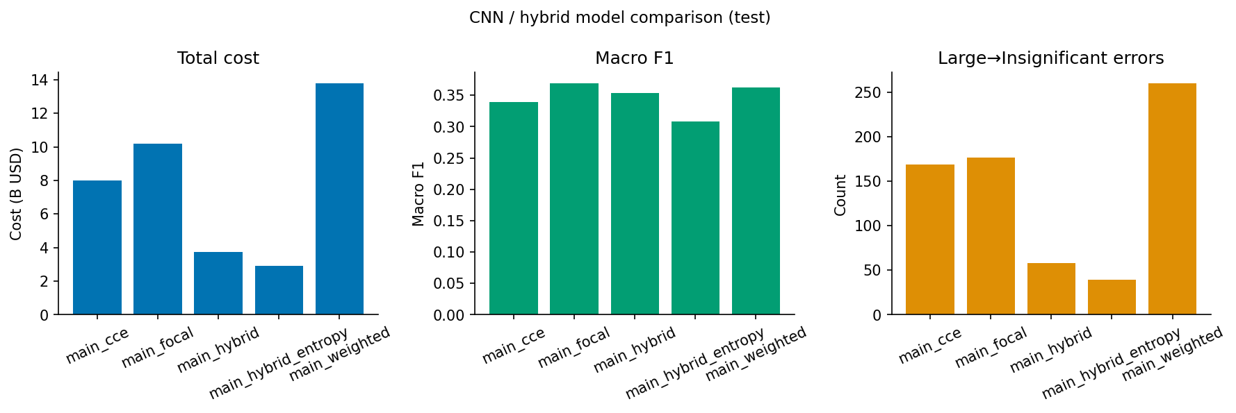
Our baseline CNN trained with CCE achieved 62.2% accuracy across all four fire severity classes after early stopping. It also recalled 81.1% of Large fires, yet 169 Large fires were predicted as Insignificant. In its current form, the CCE model collapses into the Insignificant and Large categories and predicts basically no images as Small and Medium fires. The simulated cost based on the cost matrix was $7.99 billion (Figure 1, Table 1).

Control Experiments

We tried to address the issue with existing loss functions without developing our own cost matrix. The focal loss model¹³ reached 53.8% accuracy, but the cost was higher than in the baseline configuration ($10.18 billion with 177 catastrophic errors). The cost based on weighted cross entropy¹²was even higher and equal to $13.77 billion with 260 catastrophic misses. It became apparent that the difference between the worst false negative ($42.5 million) and the worst false alarm ($85,000) was just too great to balance using frequency-based losses (Fig. 1, Table 1).

Baseline Comparisons

To make sure that the loss function, rather than CNN itself, affects the outcome, we trained four different non-deep learning baselines on spatially averaged spectral features following the fire grouped train-test split. The stratified dummy classifier reached 35.3% accuracy ($18.3 billion cost), logistic regression 59.2% ($9.4 billion), random forest 64.0% ($11.1 billion)²⁵, and XGBoost 65.3% ($11.3 billion)²⁶. Tree-based classifiers were the best baselines in terms of accuracy, but they still suffered from very high costs, which did not approach our hybrid CNN cost of $2.90 billion, thus proving that under the standard training procedure, increased accuracy does not equate to reduced cost (Table 2).

Model	Accuracy	Cohen’s κ	Macro-F1	Total Cost (USD)	Catastrophic	False Alarms
Tabular baselines (spatially-averaged spectral features)
Dummy (stratified)	0.353	n/a	n/a	$18.34B	n/a	n/a
Logistic Regression	0.592	n/a	n/a	$9.37B	n/a	n/a
Random Forest	0.640	n/a	n/a	$11.12B	n/a	n/a
XGBoost	0.653	n/a	n/a	$11.28B	n/a	n/a
CNN (four-block, four-class), by loss function
CCE (baseline)	0.622	0.352	0.339	$7.99B	169	441
Weighted CCE	0.537	0.275	0.362	$13.77B	260	375
Focal (γ = 2.0)	0.538	0.289	0.369	$10.18B	177	474
Hybrid (α = 0.10)	0.533	0.284	0.354	$3.72B	58	749
Hybrid + Entropy (α=0.10, β=0.02)	0.497	0.209	0.308	$2.90B	39	861

Catastrophic = true Large fires predicted Insignificant. False Alarms = predictions of higher severity than the truth. n/a indicates a metric not computed for that baseline.

Pure Cost Model Ablation

To understand whether a cost anchor is actually necessary, we trained on cost before building the hybrid network to see whether a cost model will perform well enough without an accuracy anchor. Our ablation, along with the cost Bayes decision rule applied to the CCE model, collapses. The cost of the Bayes decision rule brings the total cost down to $92 million, but 99% of predictions are Large fires in it. The model recognized that false alarms are so inexpensive compared to missing a Large fire that it is better to predict the highest severity classes everywhere¹⁵. With our cost matrix, the cost Bayes rule would prefer the Large class when P(Large)>0.4%. This was known as probability collapse, and it validated our need for the accuracy anchor and the entropy penalty (Figure 1, Table 1).

Hybrid Model Performance

The hybrid model (α = 0.10 cost, 0.90 CCE, β = 0.02 entropy) had a total simulated cost of $2.90 billion, which represented a 63.7% decrease compared to baseline (Figure 1, Table 1). Catastrophic misses decreased from 169 to 39 cases (77% decrease). Unlike the pure cost-based model, the hybrid maintained prediction across all four classes. The accuracy of the model became 49.7%, which is worse than baseline accuracy, but the model understood that there were different economic consequences of the misclassification: It correctly classified 85.5% of Large fires (vs. 81.1% baseline) at the expense of predicting Medium and Large fires and accepting more false alarms (861 vs. 441) for low-stakes fires where over-prediction of the fire was inexpensive. The confusion matrix (Figure 2) confirmed that the probabilities of prediction were skewed towards the classes with greater severity. The reduced accuracy is to be expected, since the cost function, rather than the error count function, was used. While standard accuracy treats the missed Large fire as equally important as the missed Insignificant fire, the model knew the difference between those two cases.

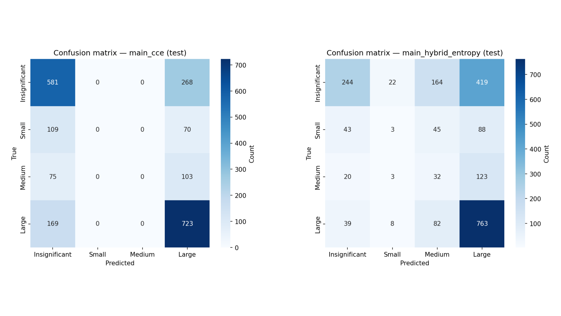
Since we are training the model to minimize cost, we use metrics that are not related to cost on the same test set to prevent circular comparison. The hybrid model got Cohen’s kappa 0.21, macro F1 0.31, Brier score 0.63, and expected calibration error (ECE) 0.039, compared to the baseline model’s CCE kappa 0.35, macro F1 0.34, Brier 0.53, and ECE 0.064. The hybrid model lost some agreement and calibration accuracy for cost and catastrophic misses reduction. Recall per class on the test set was 0.29 (Insignificant), 0.02 (Small), 0.18 (Medium), and 0.86 (Large).

We define a primary catastrophic miss as a case when a true Large fire was predicted as an Insignificant one, with secondary tiers when the true Large fire was predicted as a Small or Medium fire. Since the CCE baseline model predicts almost no Small or Medium fires, almost all 169 of its misses are in the first tier. The hybrid distributes its Large misses into three classes: Insignificant (39), Small (8), and Medium (82). Which means reducing the most costly primary tier by 77%.

Alpha and Beta Tuning

The optimization of α and β was done using grid search on the validation data only (α ∈ {0.1–0.5}, β ∈ {0, 0.02, 0.05}) using the configuration that had the minimum cost, but subject to the degeneracy filter of having at least 3 classes. The optimal α = 0.10, β = 0.02 combination was evaluated only once on the held-out test set (Table 1).

Statistical Analysis

Four statistical analysis tests were used to see if the hybrid model was actually better(Table 2). Bootstrap sampling with 1,000 iterations showed 95% CI’s of mean cost per image: baseline model $3.35M – $4.30M, hybrid model $1.12M – $1.65M. These intervals do not overlap, meaning the difference in these models is statistically significant. The permutation test with 5,000 permutations gave p<0.000001. Likewise, the Fisher exact test for large fire detection gave p = 0.013, and the Mann-Whitney U test proves lower cost per fire for the hybrid with p<0.001. All the above tests were done on this single fire grouped split, while the hyperparameters were optimized on the validation set before the test set evaluation.

Test	Statistic / Result	p-value
Permutation test (5,000 permutations)	Observed cost savings = $5.09B	< 0.000001
Fisher’s exact (Large detection 2×2)	Hybrid catches more Large fires	0.013
Mann-Whitney U (per-image cost)	Hybrid per-image cost stochastically lower	2 × 10-38
Bootstrap 95% CI, CCE baseline	Mean per-image cost $3.81M (95% CI $3.35M to $4.30M)	n/a
Bootstrap 95% CI, Hybrid	Mean per-image cost $1.38M (95% CI $1.12M to $1.65M)	n/a

All tests are based off the single fire-grouped split. Hyperparameters were selected on the validation set prior to test evaluation. A 2021 temporal holdout gives us similar results validating our results (62.5% cost reduction and catastrophic misses 954 to 148).

Monte Carlo Robustness

The hybrid won 1,998 out of 2,000 experiments (99.9%-winning rate), with median savings of 63.6% (5th percentile 50.1%, 95th percentile 70.2%) (Figure 3). Even in the case that our cost estimates are way off, the hybrid wins almost always.

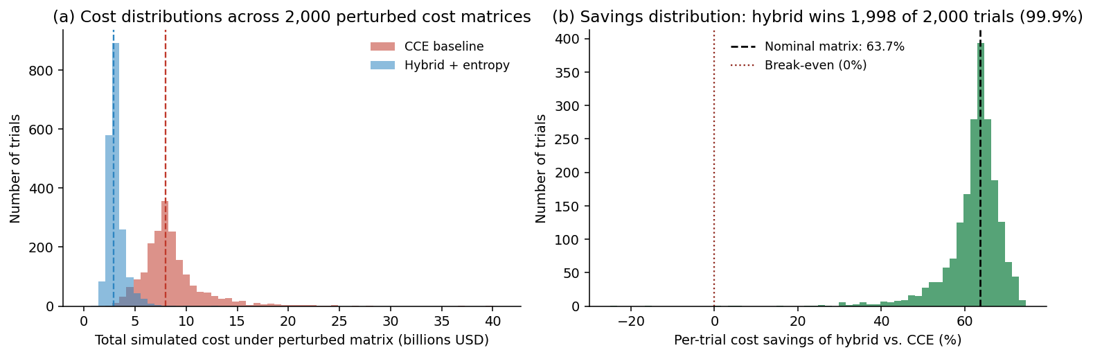
A temporal holdout (holdout of all 2021 fires) independently validated the Hybrid model, where cost fell 62.5% ($43.2B → $16.2B) and catastrophic misses fell from 954 to 148.

Discussion

Analysis of Findings

Our results confirm our initial hypothesis that accuracy optimized wildfire classifiers consistently fail to account for rare, high-cost events. This further proves that incorporating economic losses into the loss function decreases the total estimated cost. Hybrid loss decreased cost by 63.7% ($7.99B to $2.90B) and reduced the catastrophic misclassification rate from 169 to 39.

Implications and Significance

Our results show that simply optimizing for accuracy is inadequate in a setting where some errors cost more than others. The limitations of focal loss and weighted cross-entropy were shown. Focal loss worsened the situation, raising total cost to $10.18 billion because it continues optimizing for accuracy but in a less drastic manner¹³. Weighted cross entropy produced the worst results at $13.77 billion, with 260 catastrophic misclassifications. These losses are shown for the distribution of training samples instead of just the associated cost of different mistakes. Avoiding the accuracy trap requires going beyond the accuracy loss paradigm.

Pure cost loss ablation revealed a necessary trade-off: training solely on cost results in probability collapse, which is known to occur in cost-sensitive learning¹⁵, and occurs even in the high-dimensional satellite image data in our study. The use of 10% accuracy anchor and entropy loss in the hybrid loss prevented such a collapse. We differentiate two types of collapse: model collapse, which can occur during training as a result of optimization on cost loss, resulting in probability mass being shifted entirely to the most costly class (prevented by entropy loss), and decision rule degeneracy, which causes the cost Bayes rule to predict Large fires exclusively (counteracted by using argmax)²³.

Cost savings largely come from large fires. This is because the hybrid model nearly eliminates  the most costly mistake (catastrophic misclassifications) at the expense of less costly ones (increased false positives on small fires). The results of the 2021 temporal holdout experiment confirm this pattern (62.5% cost reduction).

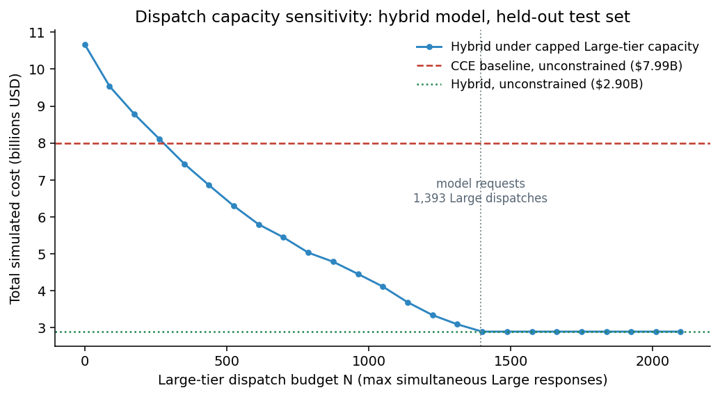
These false alarms have tangible consequences: every overcall is an unnecessary dispatch or evacuation. By raising the rate of over-severity false alarms from 441 to 861, the hybrid will make more dispatches and warnings compared to the baseline approach. An analysis of the dispatch budget puts the capacity problem into perspective (Figure 4). Here, we limit the number of simultaneous Large-tier dispatches to the budget N, and downgrade the least certain excess Large predictions to the next best class. The hybrid produces 1,393 Large dispatches out of 2,098 test images; its cost with unconstrained capacity is $2.90 billion, growing to $4.12 billion for half capacity (N = 1,049), and to $6.30 billion for quarter capacity (N = 524). In all cases where at least 350 Large tier spots are available, the hybrid is less expensive than the unconstrained CCE baseline costing $7.99 billion. At the same time, catastrophic misses of the hybrid model are still 39 for any budget higher than 87. So we conclude the trade-off is agency dependent: services that have large enough dispatch numbers would benefit from lower catastrophic misses, and others may prefer to use a cost matrix that has heavier penalties for over-response. The hybrid correctly escalates Large fires not detected by the baseline and overcalls at smaller or insignificant fire scenes. Finally, since the predictions of the model are just probabilities and not the actual dispatch decisions themselves, the costs are simulated assuming operator actions on all predictions. In reality, there should be human judgment, multi-source information fusion, and the 1–2 days latency of satellite overpasses.

Connection to Objectives

We successfully completed all of our objectives. The asymmetric cost matrix shows the inherent difference between false negatives and false alarms in wildfire detection. The hybrid model was the best model as it achieved the smallest total cost for all CNN configurations we tested. Focal loss, weighted cross entropy, and cost matrix learning failed to match the performance of the hybrid with respect to both cost and non-degeneracy. Monte Carlo simulation confirmed robustness to various assumptions about costs.

Recommendations

The accuracy trap is an issue applicable to any application domain where errors are not symmetric in their cost, including the fields of cancer screening, flood prediction, and credit default detection, among others. Models optimizing accuracy metrics will invariably suffer from performance on rare high-consequence events since these errors were simply never considered during training. Our hybrid loss only requires the specification of a cost matrix and the addition of a new weighted term to an existing loss function, making the adaptation to other tasks straightforward. Future research should seek to apply this approach in at least another domain and scale up to Vision Transformer architectures with GPU training to assess whether spatial context may further enhance the cost sensitivity of classification problems²⁷.

Limitations

A few limitations are worth noting. First, the cost matrix values were estimated using public data from average fire costs, not exact per fire figures, though the Monte Carlo analysis showed the hybrid won 99.9% of 2,000 randomly varied scenarios. Second, we only give a single fire grouped split in addition to a 2021 temporal holdout and do not test all possible combinations of fires within our dataset, or provide external validation. Due to CPU limits, full k-fold cross-validation is planned for the future. Third, severity labels carry label noise (mixed pixels, subpixel fires, cloud contamination), making the work less accurate. All dollar totals are simulations conditional on the cost matrix and do not reflect their actual damage in the real world. Fourth, severity classes based on burned pixel counts are proxies; comparing them against official NIFC severity ratings would provide stronger validation. Fifth, the Monte Carlo analysis does not retrain the model itself. It does not test the robustness of the model itself, but of the cost metric, because retraining for thousands of matrices was infeasible. Finally, our results are limited to wildfires in the United States in WildfireSpreadTS, while transfer to other locations, fuels, and fire domains is still untested.

Conclusions

Fire seasons continue to worsen, and catastrophic fire events continue to happen. It is simply not enough to train classification algorithms for accuracy alone when some errors cost much more than others. Algorithms that give higher importance to hazardous errors than overall accuracy can alter resource allocation in early fire detection: our hybrid loss function is an adaptive approach to this problem.

Appendix

All source code is publicly available at: https://github.com/Stava-Java/wildfire-cost

References

1. Munich Re. Wildfires: an accelerating risk. Munich Re NatCatSERVICE. https://www.munichre.com/en/risks/natural-disasters/wildfires.html. Accessed 15 January 2026. [↩] [↩]
2. K. Hoover. Federal wildfire management: ten-year funding trends and issues (FY2011–FY2020). Congressional Research Service, R46583, 28 October 2020. [↩] [↩]
3. National Interagency Fire Center. Total wildland fires and acres (1983–2024). NIFC Statistics. https://www.nifc.gov/fire-information/statistics. Accessed 10 January 2026. [↩] [↩] [↩]
4. USFS. Wildfire risk to communities. U.S. Forest Service, 2022. https://wildfirerisk.org/. Accessed 12 January 2026. [↩]
5. P. Jain, S. C. P. Coogan, S. G. Subramanian, M. Crowley, S. Taylor, M. D. Flannigan. A review of machine learning applications in wildfire science and management. Environmental Reviews. Vol. 28, no. 4, pg. 478–505, 2020. [↩]
6. I. Papakis, V. Linardos, M. Drakaki. A multimodal ensemble deep learning model for wildfire prediction in Greece. Remote Sensing. Vol. 17, no. 19, pg. 3310, 2025. [↩]
7. Y. Ban, P. Zhang, A. Nascetti, A. R. Bevington, M. A. Wulder. Near real time wildfire progression monitoring with Sentinel 1 SAR time series and deep learning. Scientific Reports. Vol. 10, no. 1, pg. 1322, 2020. [↩]
8. M. M. Pinto, R. Libonati, R. M. Trigo, I. F. Trigo, C. C. DaCamara. A deep learning approach for mapping and dating burned areas from Sentinel 2 data. ISPRS Journal of Photogrammetry and Remote Sensing. Vol. 160, pg. 260–274, 2020. [↩]
9. F. Huot, R. L. Hu, N. Goyal, T. Sankar, M. Ihme, Y. Chen. Next day wildfire spread: a machine learning dataset to predict wildfire spreading from remote sensing data. IEEE TGRS. Vol. 60, pg. 1–13, 2022. [↩]
10. S. Kondylatos, I. Prapas, M. Ronco, I. Papoutsis, G. Camps Valls, M. Piles, M. Á. Fernández Torres, N. Carvalhais. Wildfire danger prediction and understanding with deep learning. Geophysical Research Letters. Vol. 49, e2022GL099368, 2022. [↩]
11. S. Gerard, Y. Zhao, J. Sullivan. WildfireSpreadTS: a dataset of multi modal multi temporal satellite images for wildfire spread prediction. Zenodo, 2023. https://doi.org/10.5281/zenodo.8006177. [↩] [↩] [↩]
12. I. Goodfellow, Y. Bengio, A. Courville. Deep learning. MIT Press, 2016, pg. 170–175. [↩] [↩]
13. T. Lin, P. Goyal, R. Girshick, K. He, P. Dollár. Focal loss for dense object detection. Proceedings of the IEEE ICCV, pg. 2980–2988, 2017. [↩] [↩] [↩] [↩]
14. F. Provost, T. Fawcett, R. Kohavi. The case against accuracy estimation for comparing induction algorithms. ICML, pg. 445–453, 1998. [↩]
15. C. Elkan. The foundations of cost sensitive learning. IJCAI, pg. 973–978, 2001. [↩] [↩] [↩] [↩]
16. S. Khan, M. Hayat, M. Bennamoun, F. Sohel, R. Togneri. Cost sensitive learning of deep feature representations from imbalanced data. IEEE TNNLS. Vol. 29, no. 8, pg. 3573–3587, 2018. [↩] [↩]
17. National Wildfire Coordinating Group. NWCG fire size classes. https://www.nwcg.gov/term/glossary/size-class-of-fire. Accessed 12 January 2026. [↩]
18. D. S. Thomas, D. T. Butry, S. W. Gilbert, D. H. Webb, J. F. Fung. The costs and losses of wildfires: a literature review. NIST Special Publication 1215, 2017. [↩]
19. C. Guo, G. Pleiss, Y. Sun, K. Q. Weinberger. On calibration of modern neural networks. ICML, pg. 1321–1330, 2017. [↩]
20. M. P. Naeini, G. F. Cooper, M. Hauskrecht. Obtaining well calibrated probabilities using Bayesian binning. AAAI, pg. 2901–2907, 2015. [↩]
21. N. Chawla, K. Bowyer, L. Hall, W. Kegelmeyer. SMOTE: synthetic minority over sampling technique. JAIR. Vol. 16, pg. 321–357, 2002. [↩]
22. S. Patel, M. I. Senthil Kumar. wildfire cost. GitHub, 2026. https://github.com/Stava-Java/wildfire-cost. [↩]
23. G. Pereyra, G. Tucker, J. Chorowski, Ł. Kaiser, G. Hinton. Regularizing neural networks by penalizing confident output distributions. ICLR Workshop, arXiv:1701.06548, 2017. [↩] [↩]
24. P. I. Good. Permutation, parametric, and bootstrap tests of hypotheses. 3rd ed., Springer, 2005. [↩]
25. L. Breiman. Random forests. Machine Learning. Vol. 45, no. 1, pg. 5–32, 2001. [↩] [↩]
26. T. Chen, C. Guestrin. XGBoost: a scalable tree boosting system. Proceedings of the 22nd ACM SIGKDD, pg. 785–794, 2016. [↩] [↩]
27. A. Dosovitskiy et al. An image is worth 16×16 words: transformers for image recognition at scale. ICLR, 2021. [↩]