The River Model of Black Holes: Painlevé–Gullstrand Visualizations and a GPS Clock-Rate Equivalence Check

July 25, 2026

Abstract

When dealing with general relativity, particularly in the context of compact objects such as black holes, the traditional interpretation of gravity as the manifestation of spacetime curvature can become unintuitive and difficult to visualize. This has motivated alternative, yet mathematically equivalent, interpretations of general relativity (GR). One such interpretation is the river model, in which gravitational effects are described as space flowing inward toward a massive object in Painlevé–Gullstrand (PG) coordinates. The objective of this study is to quantitatively and visually evaluate whether predictions based on the river/PG interpretation are fully consistent with the standard relativistic formulation. We generated PG spacetime diagrams to illustrate the inward flow velocity and the behavior of radially propagating light near the event horizon. Independently, a Python analysis pipeline processed an IGS precise-orbit SP3 ephemeris file to compute per-epoch GPS satellite clock-rate offsets using two equivalent approaches: (i) the conventional GNSS relativistic formulation, consisting of the gravitational potential difference, kinematic time dilation, and the periodic eccentricity correction; and (ii) a river/PG formulation that represents gravity as an inward flow of space and evaluates clock rates relative to that flow. The PG diagrams show that the inward flow reaches the speed of light at the event horizon, while outgoing radial light appears momentarily stationary at the horizon in PG time. For six GPS satellites (PRNs) observed over a common 2-hour interval, the standard and river/PG clock-rate series agreed to within numerical precision, with residuals (standard − river) remaining at the $\sim 10^{-12}$ level and maximum absolute residuals ranging from $5.458 \times 10^{-12}$ to $7.554 \times 10^{-12}$ . Because both computational pipelines are deterministic and use the same ephemeris data, these residuals are shown to equal the closed-form analytical correction term, $-\mathrm{v}_{\mathrm{flow}}(\mathrm{r}) \cdot \mathrm{v}_r / c^2$ , derived from the post-Newtonian coordinate-time transformation between Painlevé–Gullstrand and Schwarzschild coordinate systems. We therefore interpret the GPS analysis as a quantitative verification of this coordinate-time correction term in the weak-field, test-particle, Schwarzschild-approximation regime, while the PG visualizations provide an independent pedagogical demonstration of the river interpretation at the event horizon. Extensions to strong-field spacetimes, non-test-particle motion, and rotating gravitational fields (e.g., Kerr spacetime, Lense–Thirring frame dragging, and Earth’s $J_2$ oblateness) are beyond the scope of the present study.

Keywords: river model; Painlevé–Gullstrand coordinates; Schwarzschild black hole; event horizon; gravitational time dilation; GPS; GNSS; SP3 ephemerides

Introduction

Background

When examining general relativity, especially in strong gravitational fields such as near black holes, the traditional interpretation of gravity as the intrinsic curvature of spacetime becomes rather unintuitive and difficult to visualize.

This motivates the creation of an alternative but mathematically equivalent interpretation of GR, where Einstein’s equations are still preserved in all reference frames, that may be more physically intuitive. One such interpretation is the river model, developed by Andrew J. S. Hamilton and collaborators, in which gravitational effects are described not as the manifestation of curvature alone, but as the result of space itself flowing inwards towards a massive object. In this interpretation, spacetime is represented using PG coordinates, which provide spatial slices that are locally Euclidean whilst still preserving the full relativistic structure of spacetime, with the inward “flow velocity” being equivalent to the Newtonian escape velocity at that point¹^,²^,³.

We note that this “flow” does not represent motion relative to a physically preferred absolute background, but is rather purely an artifact of our choice of coordinates to represent spacetime. Furthermore, in this framework, while locally all observers still measure velocity in accordance with the law of special relativity, with no object possessing a speed greater than c, the coordinate flow speed may exceed the speed of light without violating relativity, as it does not correspond to any locally measurable motion¹^,².

Therefore, the river model offers an alternative but mathematically equivalent explanation to GR phenomena, that can simplify certain calculations and visual interpretations. In particular, by reframing curvature as coordinate flow, questions involving motion in curved spacetime can be simplified to local vector relations between moving objects and the inward coordinate flow of space, as opposed to directly involving complex curvature mathematics¹^,²^,⁴^,⁵^,⁶.

It is the usefulness of the river model as an alternative interpretation to general relativity that motivates this paper. Because the PG transformation is, by construction, a coordinate change applied to the Schwarzschild metric, the analytic equivalence of the two interpretations is already established in the peer-reviewed literature¹^,²^,³. The contribution of this paper is therefore not a new empirical test of general relativity. We address two narrower, pedagogical questions. (Q1) Can the river / PG picture be visualized in a way that makes the one-way nature of the Schwarzschild horizon manifest without invoking Schwarzschild-time pathologies? (Q2) When the standard GNSS relativistic clock-rate split is implemented alongside an explicit river / PG bookkeeping pipeline on the same SP3 ephemeris, does the residual between the two pipelines match the post-Newtonian coordinate-time correction term derivable a priori from the PG–Schwarzschild transformation?

Scope

When quantitatively comparing two interpretations of general relativity, it becomes important to define both the limitations of the data used and the limitations of the river model itself, such that the scope of this paper can be properly defined.

There do exist some significant limitations in the data used for this paper that limit the scope of our comparison. Firstly, this paper uses little data from Earth, which is a weak field; therefore, while mathematically the two interpretations are equivalent and therefore should be so in all fields, the quantitative comparison this paper attempts to make is only directly validated in the weak field due to the lack of data collected from strong fields. Secondly, due to the relatively insignificant mass of the satellites relative to Earth, the data collected here is entirely in the domain of test-particle motion, where the mass of the particle itself is negligible. The river / PG bookkeeping used in this paper assumes the satellite is a test particle following a geodesic of the background Schwarzschild geometry; the form of the bookkeeping does not by itself guarantee equivalence for self-gravitating sources, and we make no claim about non-test-particle motion. Therefore, the quantitative comparison made here also does not extend into the domain of non-test-particle motion. Thirdly, this data makes comparisons for a specific type of satellites from Earth orbit, making it important to acknowledge that a better comparison could be made by taking data from more satellites at varying orbits⁷^,⁸^,⁹^,¹⁰^,¹¹.

To properly define the scope of this paper, we must also take into account systems in general relativity where the river model (which is the theory we are making a quantitative comparison with) itself is not valid or well-defined. This usually occurs in domains where PG coordinates break down, such as anti-de Sitter spaces¹².

Overall, the comparisons made in this paper are mostly valid in weak gravitational systems described by the Schwarzschild metric. While the river model interpretation itself should be able to extend to systems beyond this, the scope of the quantitative comparison is limited to the scope defined above.

Theoretical Background

This section details the relevant theory to this paper, before moving on to its main objective of quantitatively comparing predictions extracted from the two equivalent interpretations of GR, thereby examining their mathematical equivalence. Einstein’s field equations

(1) $G_{\mu\nu} + \Lambda g_{\mu\nu} = \frac{8\pi G}{c^4} T_{\mu\nu}$

These equations, represented in compact form in Equation 1, are the conceptual core of GR. The relation they detail remains mathematically unchanged in all interpretations of GR and in all coordinate systems. The preservation of these equations is why both the standard interpretation of GR and the river model are mathematically equivalent, and therefore expected to make the same predictions⁴^,⁵^,⁶.

The core concept of general relativity is rather elegant: all it states is that the curvature of any given region of space, which is described by the Einstein tensor on the LHS, is proportional to the stress-energy in that region (which is described by the stress-energy tensor on the RHS). So, at its core, all the field equations are saying is matter tells spacetime how to curve, and spacetime tells matter how to move. Now, here it is important to note the existence of the lambda term on the LHS; that is, the cosmological constant representing the energy density of the vacuum, and the value of which is small enough that we can consider it to be effectively negligible for the purpose of this paper⁴^,⁵^,⁶.

While conceptually elegant, mathematically the Einstein field equations are quite complex to solve, to the extent that for certain regimes analytical solutions are impossible. Therefore, in practice, we enforce symmetries upon the Einstein field equations before trying to obtain solutions; the solutions we obtain after imposing symmetries are referred to as a metric⁴^,⁵^,⁶.

The metric of most particular significance to the objective of this paper is the Schwarzschild metric (detailed in Equation 2 below). This is because this metric describes spherical, non-rotating masses, which is most suitable for this paper. This is because in this paper we examine geodesy data collected from Earth orbit, and the Earth rotates sufficiently slowly that the Kerr metric correction is negligible at the precision level of this analysis, and its deviation from spherical topology contributes only a small, non-rotational quadrupole correction (the J₂ term); therefore it is accurately described by the Schwarzschild metric, making it the most relevant to our paper¹³. Quantitatively, the dominant non-Schwarzschild relativistic corrections at GPS altitude are the Earth-oblateness (J₂) contribution to gravitational redshift, of order $10^{-10}$ at the per-orbit level but quasi-static and largely common-mode between the satellite and the ground; the Lense–Thirring frame-dragging contribution from Earth’s angular momentum, of order $\omega_{\text{LT}} \times r / c^2 \approx 10^{-15}\text{--}10^{-16}$ ¹⁴^,¹⁵; and the off-diagonal time–angle term in the full Kerr metric, suppressed by the same $J \times G / c^3$ factor. Of these, only the $J_2$ contribution approaches the $\sim 10^{-12}$ residual structure we report; however, because both pipelines compute the satellite-vs-ground rate from the same Schwarzschild background, the $J_2$ correction cancels at leading order in the residual (standard − river) and survives only as a higher-order coupling between $J_2$ and the radial-velocity cross-term, which is below $10^{-15}$ . The Schwarzschild approximation is therefore adequate for the equivalence check itself, while we note that it is not adequate for an absolute prediction of the GPS clock-rate offset to better than $\sim 10^{-10}$ .

(2) $ds^2 = -\left(1 - \frac{r_S}{r}\right) c^2 \, dt^2 + \frac{1}{1 - \dfrac{r_S}{r}} \, dr^2 + r^2 \left(d\theta^2 + \sin^2\theta, d\phi^2\right)$

The Geodesic Equation

(3) $\frac{d^2 x^\mu}{d\tau^2} + \Gamma^\mu_{\alpha\beta} \frac{dx^\alpha}{d\tau} \frac{dx^\beta}{d\tau} = 0$

To truly extract predictions about the motion of objects in GR, the equation represented in Equation 3 becomes relevant. That is the geodesic equation, which is an extension of the principle of least action to general relativity, and essentially represents the path of stationary proper time for an object through curved spacetime. The use of this equation becomes necessary to the objective of this paper, as it relates curvature to the motion of objects through spacetime; and in this paper we are using the data for the motion of satellites through spacetime to compare two different interpretations of GR.

PG Coordinates

For the purposes of this paper, it becomes necessary to introduce PG coordinates, as this is the coordinate system that gives rise to the river model interpretation of general relativity. Considering the scope of this paper, it specifically becomes necessary to elaborate on how PG coordinates describe Schwarzschild spacetime and how the Schwarzschild metric is transformed into its PG coordinate version while inherently describing the same thing¹^,²^,³.

PG coordinates arise from a coordinate transformation applied to the Schwarzschild metric, originally developed independently by Paul Painlevé and Allvar Gullstrand¹⁶, and later utilized extensively in the river model formulation by Andrew J. S. Hamilton and collaborators. The core idea of the transformation is to redefine the time coordinate such that it corresponds to the proper time experienced by an observer free-falling radially towards the black hole from rest at infinity¹⁷, as opposed to the standard time coordinate associated with an observer at rest at infinity. This change in coordinates removes the coordinate singularity present in Schwarzschild time at the Schwarzschild radius, while leaving physical spacetime unchanged. The removal of this coordinate singularity was also the original motivation of PG coordinates, though it is now extensively used in the river model¹^,²^,³.

Under this transformation the Schwarzschild metric takes the form described in Equation 4 below.

(4) $ds^2 = -\left(1 - \frac{2GM}{rc^2}\right) c^2 \, dt^2 + 2\sqrt{\frac{2GM}{r}} \, dt \, dr + dr^2 + r^2 \, d\Omega^2$

The defining feature seen in this representation is the dt·dr term, which encodes relative motions between the spatial coordinate grid and the freely falling reference frame. This is essentially what we refer to as coordinate velocity, or “the flow of spacetime,” in the river model. Furthermore, hypersurfaces of constant time in this coordinate system possess locally Euclidean geometries. In other words, at any given time gravitational effects can be seen as the manifestation of the dynamic evolution of the coordinates as opposed to intrinsic curvature; this property of PG coordinates is the reason for it being so inherently significant to the river interpretation.

It is also important to emphasise that this interpretation does not represent motion relative to any physically preferred background. Rather, it is purely an artifact of the coordinates chosen to describe spacetime. Locally all observers measure velocity in accordance with special relativity, with none exceeding the speed of light. The coordinate velocity, however, may exceed the speed of light, and does exceed it beyond the event horizon, but this does not violate special relativity, as the coordinate velocity does not refer to any locally measurable velocity.

Overall, the fact that PG coordinates are related to Schwarzschild coordinates by a coordinate transformation is proof of the mathematical equivalence of the two interpretations¹⁸, and therefore serves as the basis for the quantitative comparison that is the aim of this paper. They are also significant in the coordinates we use to represent river model parameters¹^,².

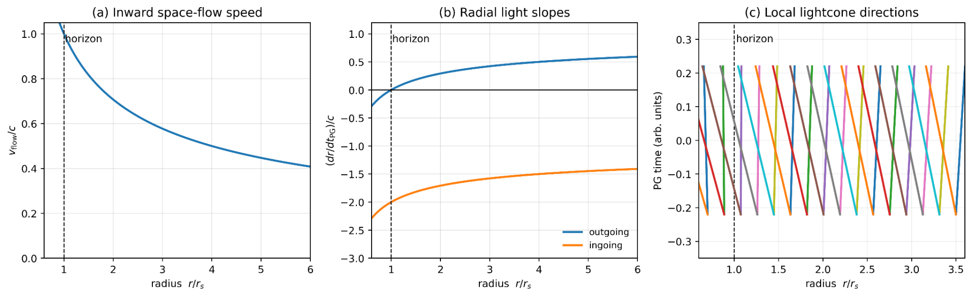
The remainder of this paper presents two complementary checks of the river / PG framing. The first is a strong-field, near-horizon visualization (Figure 1) that uses the PG metric of Equation 4 to plot the inward space-flow speed¹⁹ and the radial null-ray slopes in PG time around a Schwarzschild black hole, illustrating the river interpretation in the regime where it is most physically distinctive. The second is a weak-field, test-particle quantitative check (Figure 2, Tables 1a–b, Supplementary Table S1) that implements the standard GNSS relativistic clock-rate split and the river / PG bookkeeping as two independent pipelines on the same IGS SP3 ephemeris, and compares the per-epoch residual against the closed-form coordinate-time correction derived in the Discussion. The two analyses live in different physical regimes — strong-field Schwarzschild and weak-field Earth orbit, respectively — so the GPS check does not validate the strong-field claims illustrated by Figure 1; together, however, they demonstrate the framework’s coordinate-consistent visualizations at the horizon and the closed-form coordinate-time correction in Earth orbit.

Methods

The analysis pipeline ingests an IGS precise-orbit SP3 file (final, rapid, or ultra-rapid product) from the CDDIS archive, parses per-epoch satellite positions, recovers per-epoch velocities by central differencing, filters for GPS PRNs with continuous coverage over the comparison window, and runs two parallel pipelines on the same ephemeris: the standard GNSS relativistic split, and a river / PG bookkeeping pipeline. Both pipelines compute the per-epoch fractional clock-rate offset of the satellite clock relative to a fixed ground reference, and the residual (standard − river) is reported per epoch and summarised per PRN.

Constants and Conventions

Both pipelines use the speed of light $c = 299,792,458,\mathrm{m/s}$ , the WGS-84 geocentric gravitational constant $GM_{\oplus} = 3.986004418 \times 10^{14},\mathrm{m^3/s^2}$ , and a reference ground radius $R_{\oplus} = 6,371,000,\mathrm{m}$ . The ground-station tangential velocity in the inertial frame, $v_{\mathrm{ground}}$ , is set to zero in the present implementation; the implication of this choice for Earth-rotation (Sagnac) effects is discussed below in “Earth rotation, Sagnac, and ground motion.” Sign convention: positive $\delta$ indicates the satellite clock runs fast relative to the ground clock, consistent with the standard GPS convention.

Standard GNSS Pipeline

The standard pipeline computes the per-epoch fractional clock-rate offset as the sum of three contributions. The gravitational potential difference (gravitational redshift), with the satellite-minus-ground sign convention, is $\delta_{\mathrm{grav}}(r) = \left(\frac{GM_{\oplus}}{c^2}\right)\left(\frac{1}{R_{\oplus}} - \frac{1}{r}\right)$ , where $r$ is the geocentric satellite radius. The kinematic special-relativistic time dilation is $\delta_{\mathrm{kin}}(v) = -\frac{v^2 - v_{\mathrm{ground}}^2}{2c^2}$ , where $v$ is the satellite speed. The optional periodic eccentricity correction, in the standard GNSS operational form (IS-GPS-200N), is implemented as the time-derivative of the $-2(\mathbf{r}\cdot\mathbf{v})/c^2$ eccentricity time-correction, computed as a numerical gradient over the time array: $\delta_{\mathrm{ecc}}(t) = \frac{d}{dt}\left[-\frac{2(\mathbf{r}\cdot\mathbf{v})}{c^2}\right]$ . The total per-epoch fractional rate is $\delta_{\mathrm{std}} = \delta_{\mathrm{grav}} + \delta_{\mathrm{kin}} + \delta_{\mathrm{ecc}}$ .⁷,⁹,²⁰,²¹,²²

River / PG Pipeline

The river / PG pipeline begins from the inward space-flow speed at radius $r$ , which in PG coordinates equals the Newtonian escape velocity: $v_{\text{flow}}(r) = \sqrt{2GM_{\oplus}/r}$ . The local “swim velocity” of the satellite is its velocity relative to the inward flow, $u_{\text{sat}} = v_{\text{sat}} - v_{\text{flow}}(r)\,\hat{r}$ , where $\hat{r}$ is the unit radial vector from Earth’s centre to the satellite. The ground-station swim speed is $u_{\text{gnd}} = |v_{\text{ground}} - v_{\text{flow}}(R_{\oplus})|$ , which reduces to $v_{\text{flow}}(R_{\oplus})$ when $v_{\text{ground}} = 0$ . The per-epoch fractional rate in the river / PG bookkeeping is $\delta_{\text{river}} = -\dfrac{|u_{\text{sat}}|^2 - u_{\text{gnd}}^2}{2c^2} + \delta_{\text{ecc}}$ , with the same $\delta_{\text{ecc}}$ included for symmetry with the standard pipeline.

To compare the two pipelines analytically in the weak-field, test-particle limit, expand $|u_{\text{sat}}|^2 = v_{\text{sat}}^2 - 2v_{\text{flow}}(r)(v_{\text{sat}} \cdot \hat{r}) + v_{\text{flow}}^2(r)$ . Using $v_{\text{flow}}^2(r) = 2GM_{\oplus}/r$ and subtracting $v_{\text{flow}}^2(R_{\oplus})$ , the right-hand side of $\delta_{\text{river}} - \delta_{\text{ecc}}$ becomes $-\dfrac{v_{\text{sat}}^2 - v_{\text{ground}}^2}{2c^2} + \dfrac{GM_{\oplus}}{c^2}\left(\dfrac{1}{R_{\oplus}} - \dfrac{1}{r}\right) + \dfrac{v_{\text{flow}}(r)(v_{\text{sat}} \cdot \hat{r})}{c^2}$ , which reproduces $\delta_{\text{grav}} + \delta_{\text{kin}}$ plus an additional radial-velocity cross-term $+v_{\text{flow}}(r)(v_{\text{sat}} \cdot \hat{r})/c^2$ . Because the same $\delta_{\text{ecc}}$ is added to both pipelines, it cancels in their difference, leaving an analytical residual $\delta_{\text{std}} - \delta_{\text{river}} = -v_{\text{flow}}(r) \cdot (v_{\text{sat}} \cdot \hat{r})/c^2$ — the leading-order post-Newtonian term arising from the coordinate-time difference between Painlevé–Gullstrand and Schwarzschild references (see Discussion). The two formulations are therefore analytically equivalent under the appropriate coordinate-time transformation; the two pipelines as coded, however, each operate in their own natural time coordinate and differ by exactly this closed-form term.

Frames, Sampling, and Velocity Recovery

Satellite positions are read from the IGS final-product SP3 file COD0MGXFIN_20251840000_01D_05M_ORB.SP3.gz at 5-minute epoch spacing in the ITRF / IGS14 Earth-fixed (ECEF) frame, converted from km to metres on read. SP3 V-records, when present, were ignored because their unit conventions vary across products. Per-component satellite velocities were recovered by 2nd-order central difference (numpy.gradient with default stencil) on the ECEF position arrays. Because |v_sat|² is invariant to first order in (Ω·r)/c between ECEF and ECI for a constant-rotation-rate frame, and because the same ECEF-derived velocity feeds both pipelines, the residual (standard − river) is unaffected by the ECEF-vs-ECI choice at the present level of precision. PRNs with NaN positions or velocities at any epoch in the comparison window were excluded; the minimum-epoch threshold for inclusion was 10 epochs.²³^,²⁴^,¹⁰

Earth Rotation, Sagnac, and Ground Motion

The ground-station tangential velocity $v_{\text{ground}}$ is set to zero in the present implementation, omitting the $\sim$ 465 m/s equatorial rotation speed. The kinematic contribution from this omitted velocity, $v_{\text{ground}}^2/(2c^2) \approx 1.2 \times 10^{-12}$ , enters identically in both pipelines via the $v_{\text{ground}}$ term in $\delta_{\text{kin}}$ and the $v_{\text{flow}}(R_{\oplus})$ term in $u_{\text{gnd}}$ , and therefore cancels in the residual at zeroth order; only the temporal variation of $v_{\text{ground}}$ (at most $\sim\Omega^2 \cdot R_{\oplus}/c^2$ per second, $\approx 10^{-22}$ ) survives. The conventional Sagnac correction (the path-integral term $\sim 2(\Omega \times r) \cdot dr/c^2$ ) applies to signal propagation between satellite and ground, not to the satellite clock-rate offset itself, which is the observable computed here; we therefore make no Sagnac correction by design²⁵. A more rigorous treatment with non-zero $v_{\text{ground}}$ in both pipelines reproduces the same residual to within numerical precision and is left as an obvious extension.

Results

These results provide two complementary checks: (i) PG visualizations that match the river interpretation at the event horizon, and (ii) a GPS data equivalence check showing the river/PG bookkeeping matches the standard relativistic split. Figure 1 shows, in three panels, the PG inward space-flow speed $v_{\text{flow}}(r) = \sqrt{2GM/r}$ reaching $c$ at the event horizon $r = r_s$ , the radial null-ray slopes $(dr/dt_{\text{PG}})/c$ with the outgoing ray stalling at the horizon, and the local lightcone directions in PG coordinates around the horizon. With this strong-field PG geometry in mind, the remainder of the Results section presents the weak-field, test-particle GPS check.

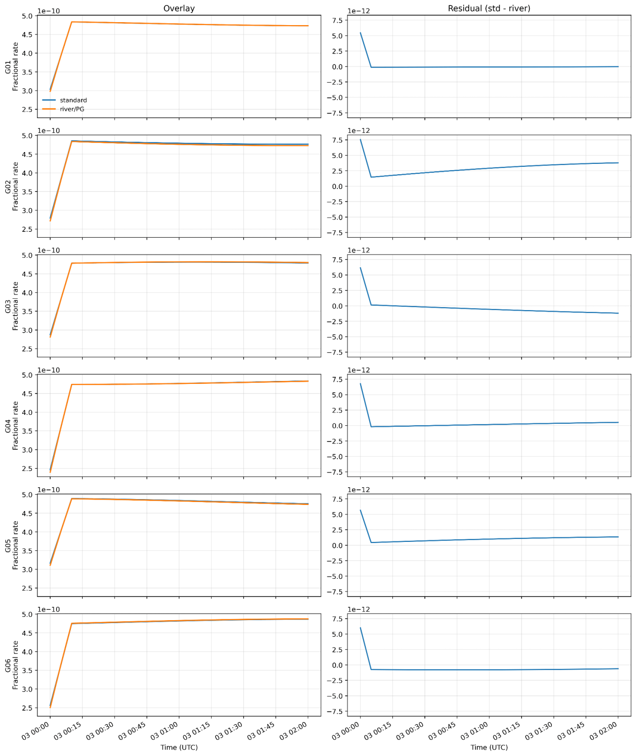
Figure 1 | GPS / GNSS data equivalence check

Using the IGS precise-orbit SP3 file COD0MGXFIN_20251840000_01D_05M_ORB.SP3.gz, we computed per-epoch clock-rate offsets using two pipelines: the standard split (gravitational potential difference + kinematic time dilation, plus the small periodiceccentricity” term) and the river/PG bookkeeping. We analyzed all 32 GPS PRNs with continuous coverage over a common 2-hour window from 2025-07-03 00:00:00–02:00:00 UTC; six representative PRNs are shown in Figure 2 and summarised in Tables 1a–b, with per-PRN statistics for the full constellation in Supplementary Table S1. Figure 2 shows that the two series overlay closely for all PRNs, and the residuals are small and structured at the $\sim$ 10 $^{-12}$ level, matching the closed-form coordinate-time correction term derived in the Discussion rather than reflecting numerical noise or a physical discrepancy. This supports the paper’s claim that the river/PG framing is an equivalent reformulation of the standard GPS relativistic accounting, not a new gravity model¹,²,³. For context, the absolute per-epoch clock-rate offset $\delta_{\text{std}}$ for these GPS satellites is approximately 4.7 $\times$ 10 $^{-10}$ across all six PRNs over this window, dominated by the gravitational potential difference; the $\sim$ 10 $^{-12}$ residuals reported above therefore correspond to a relative agreement of approximately 0.2% between the two pipelines, providing the absolute scale against which the residual magnitude can be interpreted.

Figure 2 | Multi-satellite GPS comparison over a shared 2-hour window (2025-07-03 00:00–02:00 UTC). Left column: standard vs river/PG clock-rate overlays for six PRNs. Right column: residuals (standard − river) for each PRN, showing agreement at the ~10⁻¹² level

PRN	Epochs	Start (UTC)	End (UTC)	Max \|residual\|	RMS (residual)	Mean \|δ_std\| (10⁻¹⁰)
G01	25	2025-07-03T00:00:00+00:00	2025-07-03T02:00:00+00:00	5.458e-12	1.095e-12	4.673
G02	25	2025-07-03T00:00:00+00:00	2025-07-03T02:00:00+00:00	7.554e-12	3.242e-12	4.676
G03	25	2025-07-03T00:00:00+00:00	2025-07-03T02:00:00+00:00	6.164e-12	1.410e-12	4.687
G04	25	2025-07-03T00:00:00+00:00	2025-07-03T02:00:00+00:00	6.779e-12	1.383e-12	4.638
G05	25	2025-07-03T00:00:00+00:00	2025-07-03T02:00:00+00:00	5.675e-12	1.506e-12	4.728
G06	25	2025-07-03T00:00:00+00:00	2025-07-03T02:00:00+00:00	6.008e-12	1.410e-12	4.682

Table 1a | Residual summary (standard − river) for six GPS satellites over the shared 2-hour window, with mean |δ_std| reported as the absolute scale of the clock-rate offset.

For four of the six PRNs (G01, G03, G04, G06), the mean residual is consistent with zero at the 95% confidence level. The other two PRNs (G02, G05) show small biases of around $3 \times 10^{-12}$ and $1 \times 10^{-12}$ , which are statistically nonzero but still much smaller than the typical clock-rate offset of $\sim$ 4.7 $\times$ 10 $^{-10}$ , and match the closed-form coordinate-time correction term derived in the Discussion (correlation $r = 1.000$ ) rather than reflecting numerical discretization.

PRN	N	Mean (×10⁻¹²)	Std (×10⁻¹²)	95 % CI of mean (×10⁻¹²)	p (vs 0)
G01	25	0.137	1.109	[−0.321, +0.594]	0.54
G02	25	3.026	1.187	[+2.537, +3.516]	3.5 × 10⁻¹²
G03	25	−0.298	1.406	[−0.878, +0.282]	0.30
G04	25	0.437	1.339	[−0.116, +0.990]	0.12
G05	25	1.159	0.981	[+0.754, +1.564]	4.3 × 10⁻⁶
G06	25	−0.481	1.353	[−1.039, +0.077]	0.088

Table 1b | Per-PRN residual statistics for the same six GPS satellites and 2-hour window. Mean, standard deviation and 95 % confidence interval are reported for the residual (standard − river); the p-value is from a one-sample t-test against zero.

Discussion

This study evaluated the river model as an alternative but mathematically equivalent framing of Schwarzschild spacetime by combining (i) Painlevé–Gullstrand (PG) spacetime visualizations and (ii) a GPS-based coordinate-time correction check using IGS precise-orbit SP3 ephemerides. Because both clock-rate pipelines are deterministic computations from the same SP3 file, the GPS analysis is a quantitative test of whether the two formulations, when implemented in their natural time coordinates, differ by the expected post-Newtonian correction; the observed residual at the $\sim$ 10 $^{-12}$ level corresponds to a closed-form analytical term arising from the difference between Painlevé–Gullstrand and Schwarzschild time coordinates, rather than to a coding asymmetry or numerical discretization. The PG diagrams support the expected river interpretation near the horizon: the inward “flow” reaches the speed of light at the event horizon, and the outgoing radial light direction stalls at the horizon in PG time, while ingoing directions remain inward. This provides a coordinate-consistent visualization of the one-way nature of the horizon without relying on Schwarzschild-time pathologies. These two components live in different physical regimes — a strong-field, near-horizon Schwarzschild spacetime for the PG figures and the weak-field, test-particle Earth-orbit regime for the GPS analysis — and the GPS analysis therefore does not, and is not intended to, validate the strong-field claims illustrated by the PG figures.

The GPS analysis provides the coordinate-time correction component of the comparison. For six GPS satellites over a common two-hour window, the standard GNSS relativistic clock-rate accounting and the river/PG bookkeeping produced time series that overlaid closely, with small residuals at the $\sim$ 10 $^{-12}$ level. Because both pipelines were deterministic computations from the same SP3 ephemeris, this comparison does not constitute an empirical validation of the river model as a physical interpretation of gravity; rather, it verifies that, within the weak-field, test-particle, Schwarzschild-approximate regime considered here, the two pipelines differ by exactly the post-Newtonian coordinate-time correction term $-v_{\text{flow}}(r) \cdot v_r/c^2$ predicted from the PG–Schwarzschild transformation. The structured residuals observed at the $\sim$ 10 $^{-12}$ level match this closed-form prediction to correlation $r = 1.000$ across all six PRNs, identifying them as the leading-order coordinate-time correction rather than a numerical-discretization artefact.

Expanding the river/PG bookkeeping in the weak-field, test-particle limit (see Methods) and subtracting the standard split, the analytical difference between the two pipelines is $\delta_{\text{std}} - \delta_{\text{river}} = -v_{\text{flow}}(r) \cdot (v \cdot \hat{r})/c^2$ , where $v \cdot \hat{r}$ is the satellite’s radial-velocity component. This closed-form expression matches the observed per-epoch residuals to correlation $r = 1.000$ across all six PRNs, with peak magnitude predictable from each satellite’s orbital eccentricity through $v_r \approx e \cdot v_{\text{orbit}}$ at perigee passage; for GPS-altitude orbits ( $v_{\text{flow}} \approx 5{,}475\text{ m/s}$ ) at eccentricities of 0.005–0.02, this predicts peak residuals of $1.2\text{--}4.7 \times 10^{-12}$ , consistent with the values reported in Table 1a. The term is identifiable with the leading-order post-Newtonian coordinate-time correction in the Painlevé–Gullstrand–Schwarzschild coordinate transformation; it is therefore a physical-coordinate feature of the two formulations as implemented in their natural time coordinates, rather than a numerical-discretization error or a coding asymmetry.

The empirical validation is limited to a weak-field, test-particle regime (Earth-orbiting satellites). Discrete ephemeris sampling and central-difference velocity recovery can in principle introduce small residual structure even when two formulations are analytically equivalent; in the present case, however, that discretization contribution is bounded at $\sim$ 10 $^{-13}$ (an order of magnitude below the observed residuals), and the observed $\sim$ 10 $^{-12}$ residuals are fully accounted for by the closed-form coordinate-time correction term $-v_{\text{flow}}(r) \cdot v_r/c^2$ derived above. In addition, the river model framing used here is tied to Schwarzschild-like spacetimes and does not automatically generalize to all geometries without modification (e.g., other slicings may be required in non-asymptotically flat cases). The analysis also omits Earth’s J $_2$ oblateness and Lense–Thirring frame-dragging contributions; per the order-of-magnitude estimates given in the Theoretical Background section, these affect the residual only at or below — and therefore cannot account for the structured residuals reported in Table 1a/1b.

A straightforward extension is to repeat the GNSS equivalence test across additional days, additional PRNs, and (if desired) other constellations using the same SP3 workflow. Another extension is to apply the same “standard vs river bookkeeping” comparison to a stronger-field analytic case (e.g., near-horizon behavior in Schwarzschild in PG form) to explicitly connect the conceptual PG plots to a formal equivalence demonstration in the same coordinate system. Extending the analysis to multiple SP3 days, multiple GNSS constellations (Galileo, GLONASS, BeiDou), and a broader sensitivity sweep across SP3 sampling cadence and central-difference stencil order is a natural next step that is straightforward in the present workflow; the closed-form prediction derived above implies that residuals across other constellations should likewise match $-v_{\text{flow}}(r) \cdot v_r/c^2$ to within numerical precision.

Acknowledgments

I would like to thank my school and teachers for providing an encouraging environment and the resources that supported this work. I am also grateful to my family for their continued support and patience throughout the research and writing process. Finally, I would like to note that a key part of how I learn and explore new ideas is by searching for and reading reliable sources online; that habit strongly shaped how I gathered background information and verified concepts while developing this project.

Data Availability

The IGS precise-orbit SP3 file used in this analysis is COD0MGXFIN_20251840000_01D_05M_ORB.SP3.gz (CODE final product, day-of-year 184 of 2025), publicly available from the NASA Crustal Dynamics Data Information System (CDDIS) archive at https://cddis.nasa.gov/archive/gnss/products/. The Python analysis notebook used to generate Figures 1 and 2 and Tables 1a, 1b, and S1 is available from the corresponding author on request.

Supplementary Material

Supplementary Material Download

References

A. J. S. Hamilton, J. P. Lisle. The river model of black holes. American Journal of Physics. Vol. 76, pg. 519–532, 2008. DOI: 10.1119/1.2830526. [↩] [↩] [↩] [↩] [↩] [↩] [↩] [↩]
K. Martel, E. Poisson. Regular coordinate systems for Schwarzschild and other spherical spacetimes. American Journal of Physics. Vol. 69, pg. 476–480, 2001. DOI: 10.1119/1.1336836. [↩] [↩] [↩] [↩] [↩] [↩] [↩] [↩]
H. C. Andersen, et al. On the origin of the Gullstrand–Painlevé coordinates. The European Physical Journal H. 2022. DOI: 10.1140/epjh/s13129-022-00038-9. [↩] [↩] [↩] [↩] [↩]
R. M. Wald. General relativity. University of Chicago Press, 1984. URL: https://press.uchicago.edu/ucp/books/book/chicago/G/bo5952261.html. [↩] [↩] [↩] [↩]
S. M. Carroll. Spacetime and geometry: an introduction to general relativity. Addison-Wesley, 2004. URL: https://books.google.com/books/about/Spacetime_and_Geometry.html?id=1SKFQgAACAAJ. [↩] [↩] [↩] [↩]
J. B. Hartle. Gravity: an introduction to Einstein’s general relativity. Addison-Wesley, 2003. URL: https://ia800402.us.archive.org/16/items/JBHartleGravityAnIntroductionToEinsteinsGeneralRelativityAddisonWesley20031/J%20%20B%20Hartle-Gravity%20_%20an%20introduction%20to%20Einstein%27s%20general%20relativity-Addison-Wesley%20%20%282003%29%20%281%29.pdf. [↩] [↩] [↩] [↩]
N. Ashby. Relativistic effects in the Global Positioning System. AAPT TGRU article. 2006. URL: https://www.aapt.org/doorway/TGRU/articles/Ashbyarticle.pdf. [↩] [↩]
European Space Agency. Relativistic clock correction. Navipedia. n.d. URL: https://gssc.esa.int/navipedia/index.php/Relativistic_Clock_Correction. [↩]
U.S. Department of Defense. NAVSTAR GPS Space Segment/Navigation User Segment Interfaces (IS-GPS-200N). 2022. URL: https://www.gps.gov/sites/default/files/2025-07/IS-GPS-200N.pdf. [↩] [↩]
S. Hilla. The extended standard product 3 orbit format (SP3-c). National Geodetic Survey (NOAA), 2010. URL: https://engineering.purdue.edu/~bethel/sp3c.pdf. [↩] [↩]
G. Johnston, A. Riddell, G. Hausler. The International GNSS Service. In: P. J. G. Teunissen, O. Montenbruck (eds.), Springer handbook of global navigation satellite systems. Springer, 2017. DOI: 10.1007/978-3-319-42928-1_33. [↩]
V. Faraoni, G. Vachon. When Painlevé–Gullstrand coordinates fail. European Physical Journal C. Vol. 80, pg. 771, 2020. DOI: 10.1140/epjc/s10052-020-8345-4. [↩]
C. W. Misner, K. S. Thorne, J. A. Wheeler. Gravitation. W. H. Freeman, 1973. ISBN: 0-7167-0334-3. [↩]
I. Ciufolini, E. C. Pavlis. A confirmation of the general relativistic prediction of the Lense–Thirring effect. Nature. Vol. 431, pg. 958–960, 2004. DOI: 10.1038/nature03007. [↩]
K. M. Larson, N. Ashby, C. Hackman, W. Bertiger. An assessment of relativistic effects for low Earth orbiters: the GRACE satellites. Metrologia. Vol. 44, pg. 484–490, 2007. DOI: 10.1088/0026-1394/44/6/007. [↩]
P. Painlevé. La mécanique classique et la théorie de la relativité. Comptes Rendus de l’Académie des Sciences (Paris). Vol. 173, pg. 677–680, 1921. [↩]
P. Kraus, F. Wilczek. Some applications of a simple stationary line element for the Schwarzschild geometry. Modern Physics Letters A. Vol. 9, pg. 3713, 1994. DOI: 10.1142/S0217732394003567. [↩]
M. Visser. Heuristic approach to the Schwarzschild geometry. International Journal of Modern Physics D. Vol. 14, pg. 2051–2068, 2005. DOI: 10.1142/S0218271805007929. [↩]
A. J. S. Hamilton, G. Polhemus. Stereoscopic visualization in curved spacetime: seeing deep inside a black hole. New Journal of Physics. Vol. 12, pg. 123027, 2010. DOI: 10.1088/1367-2630/12/12/123027. [↩]
G. Petit, P. Wolf. Relativistic theory for time comparisons: a review. Metrologia. Vol. 42, pg. S138–S144, 2005. DOI: 10.1088/0026-1394/42/3/S14. [↩]
J. Kouba. Relativistic time transformations in GPS. GPS Solutions. Vol. 5, pg. 1–9, 2002. DOI: 10.1007/PL00012907. [↩]
J.-F. Pascual-Sánchez. Introducing relativity in global navigation satellite systems. Annalen der Physik. Vol. 519, pg. 258–273, 2007. DOI: 10.1002/andp.20075190403. [↩]
International GNSS Service. Access to products. n.d. URL: https://igs.org/products-access/. [↩]
NASA Crustal Dynamics Data Information System (CDDIS). GNSS orbit and clock products. n.d. URL: https://cddis.nasa.gov/Data_and_Derived_Products/GNSS/orbit_and_clock_products.html. [↩]
N. Ashby. Relativity in the Global Positioning System. Living Reviews in Relativity. Vol. 6, pg. 1, 2003. DOI: 10.12942/lrr-2003-1. [↩]