Comparative Evaluation of Classical, Convolutional, and Transformer-Based Models for Crop Disease Classification

Abstract

Crop disease identification is critical for our global food security as crop diseases cost the global economy approximately $220 billion every year. While machine learning is a practical solution for classification, there has been a lack of research in comparing different architectures. This study compares four architectures for 13-class crop disease classification across four crop types using 16,323 images: logistic regression, a five-layer neural network, a custom five-block convolutional neural network (CNN), and a downscaled vision transformer (ViT). All of the models were tested with a 5-fold stratified cross-validation framework with the same data splits (80% training / 20% validation), AdamW optimization, and sample-inverse class weights. The CNN had the highest performance with a weighted F1-score of 89.68% and a macro F1-score of 89.40%. It was also the most practical for real-world use as it required a reasonable 3,702,541 parameters and had an inference speed of 47.29 ms per image. The ViT performed competitively but slightly behind the CNN architecture. It achieved a weighted F1-score of 88.92% and a macro F1-score of 88.26%. This difference in performance and the clear oscillations in our ViT’s validation loss curves suggest that self-attention layers struggle with optimization instability when trained from scratch on medium-sized datasets. Simpler models like the logistic regression and neural networks performed substantially worse with macro F1-scores of 30.31% and 59.62% respectively. Overall, CNNs provide the most dependable and practical choice for resource-limited mobile deployment.

Keywords: Crop Disease Detection, Deep Learning, Convolutional Neural Networks, Vision Transformers, Agricultural Computer Vision

Introduction

Crop disease identification is critical for ensuring our global food security with plant diseases costing the global economy approximately $220 billion annually¹. Traditional methods for diagnosing crop diseases are typically visual tests by experienced farmers or microscopic examinations that require specialized equipment. Both of these methods may be unavailable or impractical for many people living in developing regions².

Artificial intelligence is a strong and practical solution as it can be both accessible and accurate for classifying crop diseases. Convolutional Neural Networks (CNNs) have been the main architecture used due to their ability for spatial feature extraction. This allows these models to learn visual features from the images themselves. CNNs have shown high performance but are often more limited when dealing with complex datasets where there is a lot of variation within a class or similarities among different classes. Vision Transformers (ViTs) have been developed as a promising alternative to address these limitations through their use of both global and local feature extraction. This allows them to better understand more subtle differences and varying field conditions. 

Previous studies on the classification of crop diseases often focus on one architecture such as CNNs or ViTs and do not include more classical models such as logistic regression or fully connected neural networks. Evaluating these simpler models is important as they establish a baseline performance to prove if more complex models are necessary. Many of these studies also focus on a single crop dataset or the PlantVillage dataset³ that use controlled image conditions rather than true field environments. There is also little research comparing not only the performance of convolutional and transformer architectures but also the real-world applicability of these models. Additionally, in studies that do compare different models, they often use transfer learning inconsistently which can lead to unreliable comparisons.

Our study compares four machine learning architectures: logistic regression, fully connected neural networks, CNNs, and ViTs, under a consistent experimental setup. Our research also discusses the trade-offs between these different architectures in terms of accuracy, data efficiency and real-world practicality. We hypothesize that the CNN will perform better than the more traditional logistic regression and neural network models due to its specialization for image classification from its spatial feature extraction. The ViT will also likely achieve competitive but lower overall results than the CNN. This is because training these models from scratch on a mid-sized dataset of 16,323 images can greatly limit their performance compared to models that use pre-training. To help with the reproducibility of our experiment, our source code, hyperparameters, and evaluation process are accessible at: https://github.com/rohankomm-arch/crop-disease-benchmarking.

Background

While CNNs have revolutionized the automation of crop disease detection through their use of spatial inductive bias and translational invariance, their performance is still heavily dependent on their specific architectural configurations. Early multi-crop models such as the benchmark models on the PlantVillage dataset showed that standard CNNs could achieve validation accuracies up to 99.81% under uniform and strict image conditions⁴. Even more recent models have focused on improving these results under more complex scenarios. Two major examples include the EfficientNet framework⁵ that introduced compound scaling to balance network depth, width, and resolution and the ConvNeXt architecture⁶ that modernized standard convolutional layers to mimic the behaviors of transformers. CNN architectures still remain restricted by their focus on localized windows despite these improvements. Because these models process images through local kernel windows, they are far more susceptible to lower performance when differentiating similar flaws on leaves⁷.

To address these restrictions of CNNs, Dosovitskiy et al.⁸ introduced vision transformers that use multi-head self-attention mechanisms to map global connections across an entire image. ViTs are able to understand relationships between distant pixels which allows them to understand stronger connections compared to localized CNNs. However, the primary issue with ViTs is the massive amount of data they need for the self-attention layers⁹. This is because ViTs initially lack the same spatial inductive biases of CNNs. This means that they struggle to understand that neighboring pixels are more relevant to each other than farther pixels. Therefore, when ViTs are trained from scratch on mid-sized datasets, such as the 16,323 image dataset utilized in this study, they show lower data efficiency and lower performance compared to pre-trained versions. 

Due to the trade-offs between CNNs and ViTs, many more modern models have shifted towards a hybrid system between these two architectures. Modern frameworks have combined these architectures using parallel networks that merge local and global feature paths through tensor concatenation¹⁰. Some frameworks also use sequential architectures that utilize shallow convolutional stems to extract local textures before passing them to transformer layers¹¹. Additionally, to support practical in-field deployment, recent hybrid models have also incorporated layer-wise Explainable AI (XAI) diagnostics. These diagnostics use gradient-weighted class activation mapping (Grad-CAM) to match transformer attention matrices with expert-annotated disease symptoms to make sure that the model focuses on the correct plant features¹². While these complex models achieve high performances, they hide a flaw in current research in that they are rarely compared against simpler baseline models under strict, controlled training conditions. Current literature also uses a lot of inconsistent transfer learning which makes it difficult to truly compare CNNs and ViTs in their efficiency with data. In addition, for practical use on low-cost hardware, it is important to understand trade-offs such as total trainable parameter counts and inference latencies¹³. This lack of benchmark measurements shaped the experimental design of our study. An overview of architectural milestones, dataset complexity and limitations are given in Table 1.

Study	Dataset	Model	Accuracy	Gaps
Saleem et al. (2020)4	54,306 images covering 38 classes from the PlantVillage dataset. Contains 14 plant species (including Tomato, Cassava, and Maize).	18 CNN variants across 6 deep learning optimizers.	Xception backbone with the Adam optimizer got a validation accuracy of 99.81% and F1-score of 0.9978.	The Xception model required a long training time of around 3,400 seconds per epoch.
Sharma et al. (2022)14	7,432 leaf images for Rice and Potato crops.	A custom CNN Architecture tested against traditional classifiers.	Custom CNN got 99.58% accuracy on rice diseases and 97.66% accuracy on potato diseases.	Had a narrow scope of only two crops.
Ahad et al. (2023)15	Dataset covers 9 regional leaf diseases for Rice. Each disease class contains 100 images and augmentations were used to increase the dataset to 42,876 total images.	6 standard CNN models: DenseNet121, InceptionV3, MobileNetV2, ResNext101, ResNet152V, and SEResNext101.	SEResNext101 combined with Transfer Learning got an accuracy of 98.00%.	It was restricted to a single crop in rice.
Batchuluun et al. (2022)16	4,720 custom thermal images of Rice (including paddies) combined with an open database.	CNN integrated with Explainable AI (XAI) to interpret blurry thermal features.	Achieved an accuracy of 98.55% on the custom dataset and 90.04% on the Paddy dataset.	The model struggled with low quality and blurriness from the thermal images. The model was also sensitive to factors like temperature and humidity.
Sachdeva et al. (2021)17	20,639 images from PlantVillage across 15 balanced classes. Includes Potato, Tomato, and Bell Pepper crops.	A deep Residual CNN with a Bayesian learning framework.	Achieved an accuracy of 98.90%.	Had poor performance on datasets with more complex backgrounds.
Lilhore et al. (2022)18	6,256 images spanning 5 classes for Cassava.	Enhanced CNN (ECNN) that uses depth-wise separable convolutions.	The ECNN architecture got a 99.30% accuracy rate on the balanced subset.	The architecture is limited to a single crop and the dataset size is fairly restricted.
Timothy et al. (2022)19	1,050 Cashew images consisting of healthy and diseased leaf, stem, and nut images. 1750 total images including augmentations.	A standard ResNet-50 CNN tested with 5-fold cross-validation.	Achieved classification accuracy of 97.76%.	It was limited by a small, restricted dataset. It also heavily relied on high-quality, uniform images.
Karthik et al. (2024)10	Utilizes the CCMT dataset that contains 102,976 images and 22 classes for Cashew, Cassava, Maize, Tomato.	Dual-Track Architecture with a Convolutional block and a global Swin Transformer (DAMFN).	Achieved a multi-class classification accuracy of 95.68%.	The massive parameter size causes processing delays which can make it harder to run on low-cost mobile devices.
Shandilya et al. (2025)11	Maize Leaf Disease datasets from Kaggle and Mendeley.	A custom hybrid CNN-ViT framework.	Achieved validation accuracy of 99.15%.	The focus was restricted to a single crop in maize.
Paul et al. (2026)12	Mendeley Papaya Leaf Disease Dataset containing 2,500 images across 5 classes.	A hybrid CNN-Transformer framework. It also includes Grad-CAM analysis for multi-level interpretability.	Achieved 87.3% accuracy on expert-annotated disease patches.	Lack of real-world testing in true in-field conditions. Did not outperform CNN or transformer baselines.
Srinivasan et al. (2026)20	Two publicly available Kaggle datasets containing a combined total of 104,768 RGB leaf images across 18 disease classes for Corn (Maize), Potato and Tomato.	ResViT-152 which is a hybrid CNN-Vision Transformer architecture. It was compared against InceptionNetV3, ResNet152V2, ViT, and BERT models.	IntraTest accuracy: 99.12% (corn), 98.94% (tomato), 99.06% (potato); CrossTest accuracy: 96.27% (corn), 96.22% (tomato), 96.15% (potato).	The model was mainly evaluated under balanced conditions. It needs more real-world testing before practical use.
Noor et al. (2026)21	Large-scale dataset containing 32 plant disease classes. Crops are Coffee, Cotton, Cucumber, Olive, Tomato and Wheat.	YOLOv8 framework optimized by Transfer Learning.	Achieved a recall rate of 0.94 and an overall accuracy of 92.57%.	There was limited dataset diversity. The high-computational cost may also limit its use in resource-constrained regions.

Dataset

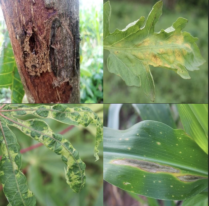
The dataset we used in our research is the Dataset for Crop Pest and Disease Detection by the University of Energy and Natural Resources in Ghana²². The dataset includes 24,881 images of four main crops: cashew, cassava, maize, and tomato. Within those classes, there are 22 subclasses with each crop having sub-datasets for various diseases and pests along with healthy versions of each crop. For our study, we used 13 sub-datasets, consisting of 9 disease and 4 healthy classes. We also discarded pest subclasses due to the fundamental differences between the visual characteristics of pest damage and disease damage. From a computer vision perspective, pest damage in crops is usually shown by bite marks, holes or surface residue from insect activity. In contrast, disease-related changes often come in different forms such as lesions, discoloration, dots, streaks or wilting. Mixing these two different issues into a single classification task can cause our models to perform worse since the training targets conflict. The final classes we chose are shown in Table 2. The total number of images in these remaining classes was 16,362 which came from 8,519 pest images being removed from the original 24,881 image total. This number was reduced even more to 16,323 because of 39 corrupted images. We filtered out these corrupted images during preprocessing to protect the stability of our training. Figure 1 also shows some sample images from the dataset.

Crop Disease	Crop Category	Number of Images
Cashew Anthracnose	Cashew	1729
Cashew Gummosis	Cashew	392
Cashew Red Rust	Cashew	1682
Cashew Healthy	Cashew	1368
Cassava Bacterial Blight	Cassava	2614
Cassava Mosaic	Cassava	1205
Cassava Healthy	Cassava	1193
Maize Leaf Blight	Maize	990
Maize Streak Virus	Maize	965
Maize Healthy	Maize	204
Tomato Septoria Leaf Spot	Tomato	2743
Tomato Verticillium Wilt	Tomato	772
Tomato Healthy	Tomato	466

We used a 5-fold stratified cross-validation setup to prevent any bias from a single train-test split and to better handle class imbalances in the dataset. The 16,323 images were split into 5 groups with the same class distribution as shown in Table 2. For each fold, one fold was used as the validation set and the other four folds were used for training. This was repeated 5 times so that every image could be used in the validation set. We also implemented z-score normalization inside each cross-validation loop. We did this to prevent data leakage, meaning that the pixel mean and standard deviation were calculated only based on the unchanged training images for each specific fold before adding any transformations. This makes sure that no pixel distributions from the validation set leak into the normalization process. The validation set was also kept completely untouched and unseen in order to provide an accurate and unbiased evaluation of the models. The dataset overall also exhibits severe class imbalance as the highest represented class, Tomato Septoria Leaf Spot, contains 2,743 images while the lowest represented, Maize Healthy, contains only 204 images. This resulted in a fairly large Imbalance Ratio of 13.45:1, which we mitigate by using sample-inverse class weighting during training.

We also chose different input sizes and data augmentations based on the different architectures of the models to allow each model to perform to the best of its capabilities. For the Logistic Regression and Neural Network models, we set the pixel resolution to 64 × 64 and did not include augmentations. This is due to how larger image resolutions would lead to larger feature vectors, causing these simpler models to easily overfit. Random rotations, shears and other augmentations could also hinder the pixel relationships that these models need to learn. For our CNN and ViT models, we used a 128 × 128 pixel resolution and data augmentation like horizontal and vertical flips, rotations and shears on the training set. These architectures require a larger image resolution as ViTs need enough pixels to create patch embeddings and CNNs need more pixels so that convolutional filters do not blur important features. Data augmentation was also necessary because both models were trained from scratch and needed increased data variety to prevent them from overfitting to the background noise in the images²³.

Methods

Training Procedure and Implementation 

We used the PyTorch framework across all the models due to its flexibility and the greater control it allows for model architectures and the training process. Our training was performed using Google Colab with GPU acceleration (NVIDIA T4) when available, as well as on a Windows machine using a CPU for the smaller models. To help with consistency, we used a random seed of 42 for all of the data splits and weight initializations. Each individual fold also isolated 20% of the data for validation and 80% for training. The specific hyperparameter configurations are outlined below in Table 3.

Model	Image Size	Epochs	Learning Rate	Batch Size
Logistic Regression	64 × 64	30	0.001	32
Neural Network	64 × 64	60	0.001	32
CNN	128 × 128	60	0.0001	32
Vision Transformer	128 × 128	60	0.0001	32

We utilized the AdamW optimizer²⁴ along with weighted cross-entropy loss for all the models to maintain fair and consistent optimization for each architecture. This loss function includes sample-inverse class weighting coefficients that are calculated from the training splits. This penalizes the models for misclassifications in the minority classes more heavily due to the dataset’s strong class imbalance. As demonstrated by Huang et al.²⁵, using class-adaptive weighting schedules in the loss function helps stabilize the model on imbalanced data which mitigates it from consistently favoring the majority classes. While the optimizer, cross-validation boundaries, and loss frameworks were consistent for all of the models, we adjusted the other hyperparameters such as learning rate, number of epochs, image resolution and model depth for each architecture individually. We tuned these parameters based on their validation performance and to account for how these models are all very structurally different. To prevent overfitting and any unnecessary processing time during the training process, we also included an early stopping mechanism with a patience of 8 epochs across all of the models. If the validation loss did not show any improvement for eight consecutive epochs, the training was ended early. The model weights were also changed back to their best-performing state. For example, the CNN and ViT typically require lower learning rates and more training epochs than the regression model due to the increased parameters and higher complexity in deeper layers. Keeping the same, identical hyperparameters for all of these different architectures would also likely hurt certain models with differing learning patterns and structural designs. Therefore, we kept the experimental control consistent for data splits, optimizer choice, loss function and evaluation metrics to maintain fair and effective training. 

Logistic Regression

We first implemented a multi-class logistic regression model to establish a performance floor for this crop disease classification task. We chose an input resolution of 64 × 64 × 3 to account for the risk of overfitting with flat, high-dimensional spaces. These inputs are flattened into a feature vector x of 12,288 dimensions. This vector is then given directly into a single fully connected linear layer that computes the raw class logits based on this equation:

where W represents the learnable parameter weights matrix, and b represents the class bias vector. These logits are then passed into the cross-entropy loss function. This computes the softmax probability distribution to update the weights using AdamW.

Neural Network

After the regression model, we implemented a deep neural network to evaluate a model with multiple layers that can understand non-linear relationships. For the neural network, we kept the image resolution at 64 × 64 × 3 pixels in order to stay consistent with the logistic regression model and reduce the risk of overfitting. These inputs are flattened into a feature vector x of 12,288 values. The data is then passed through five hidden layers to gradually shrink the feature dimensions (1024 → 768 → 512 → 256 → 128). To prevent the model from overfitting and just memorizing the training images, we added batch normalization to stabilize training and dropout layers to limit the neurons from being too dependent on each other. The architectural progression and feature transformations are shown by the following sequence:

W₁ through W₆ are the learnable weight matrices that connect the different layers while b₁ through b₆ represent the bias vectors. The size of the weight matrices also matches the shrinking structure of the network. A Rectified Linear Unit (ReLU) activation function is also used after each linear layer to help the model learn non-linear patterns. 

The final output layer turns the 128-dimensional embedding from H₅ into raw class logits across the 13 classes. These scores are then passed into the cross-entropy loss function to evaluate the probability distribution.

Convolutional Neural Network

The next model we developed was a Convolutional Neural Network, which uses local convolutional filters to recognize features like edges, lesions, and color changes. The model processes the input images at a resolution of 128 × 128 × 3 through 5 convolutional blocks, and then a dense, multi-layer classification head. Each convolutional block includes a 2D convolutional layer with a 3 × 3 kernel (and a stride and padding of 1), a 2D batch normalization layer to stabilize data distributions, a ReLU activation function to introduce non-linearity, and a 2 × 2 max pooling layer with a stride of 2. The layers, feature map dimensions, and parameter counts for the architecture are shown in Table 4.

Stage / Layer	Component Type	Kernel Size / Configuration	Output Shape (Batch, C, H, W)	Activation / Regularization
Input	Raw Image Tensor	—	(Batch, 3, 128, 128)	—
Block 1	2DConvolution	3 × 3, Stride 1, Padding 1	(Batch, 32, 128, 128)	Batch Normalization, ReLU
	Max Pooling	2 × 2, Stride 2	(Batch, 32, 64, 64)	—
Block 2	2D Convolution	3 × 3, Stride 1, Padding 1	(Batch, 64, 64, 64)	Batch Normalization, ReLU
	Max Pooling	2 × 2, Stride 2	(Batch, 64, 32, 32)	—
Block 3	2D Convolution	3 × 3, Stride 1, Padding 1	(Batch, 128, 32, 32)	Batch Normalization, ReLU
	Max Pooling	2 × 2, Stride 2	(Batch, 128, 16, 16)	—
Block 4	2D Convolution	3 × 3, Stride 1, Padding 1	(Batch, 256, 16, 16)	Batch Normalization, ReLU
	Max Pooling	2 × 2, Stride 2	(Batch, 256, 8, 8)	—
Block 5	2D Convolution	3 × 3, Stride 1, Padding 1	(Batch, 512, 8, 8)	Batch Normalization, ReLU
	Max Pooling	2 × 2, Stride 2	(Batch, 512, 4, 4)	—
Flatten	Tensor Reshaping	Flatten (dim = 1)	(Batch, 8192)	—
Dense 1	Fully Connected	8192 → 256	(Batch, 256)	ReLU, Dropout (p=0.5)
Dense 2	Fully Connected	256 → 128	(Batch, 128)	ReLU, Dropout (p=0.5)
Output Head	Fully Connected	128 → 13	(Batch, 13)	Softmax (via Loss Function)

After the final max pooling layer in Block 5, the 512 × 4 × 4 feature map is flattened into an 8,192-dimensional vector. This vector is then turned into a 256-dimensional hidden layer, which is reduced down to a 128-dimensional hidden layer. Each hidden layer is also followed by a ReLU activation and a dropout layer of p = 0.5 to prevent overfitting. The final layer turns the 128-dimensional embedding to the 13 raw class logits. These are then optimized by cross-entropy loss and the AdamW optimizer. 

For our CNN, we made multiple critical architectural design choices to optimize this network for crop disease classification. We chose smaller 3 × 3 filters instead of larger kernels, like 5 × 5 or 7 × 7 because they reduce the total parameter count while also keeping the same visual field. We also set the padding parameter to 1 to prevent the feature maps from shrinking. Our network depth of five blocks also lets the architecture learn increasingly complex features through the deeper layers. This means that the early layers learn more simple ideas like edges and textures, while the deeper layers turn these concepts into more high-level ideas like leaf shapes, spot patterns, and lesions. Finally, the 2 × 2 max pooling allows the network to understand features no matter where their pixel coordinates are on the leaf. The pooling layer also limits the computational footprint by balancing the increased depth.

Vision Transformer

We then implemented a Vision Transformer to compare global, self-attention-based architectures to localized convolutional neural networks. We gave the ViT the same image resolution as the CNN of 128 × 128 × 3. ViTs process these image inputs by dividing them into non-overlapping patches. Standard larger-scale ViTs traditionally use 16 × 16 patches on 224 × 224 inputs. However, we structured our model using a patch size of 8 × 8 on the 128 × 128 resolution which creates 256 distinct patches. Following Dosovitskiy et al.⁸, reducing the patch dimensions for more compact input resolutions allows the model to capture finer details in the image. Each individual patch is flattened and mapped by a linear projection layer into the 256-dimensional embedding space. Because transformers lack the inherent inductive bias that is needed to understand the spatial relationships between pixels, a trainable positional embedding of shape (1, 257, 256) is added to the projected tokens. This includes the 256 patch tokens plus the additional classification (CLS) token that summarizes the overall context of the image.

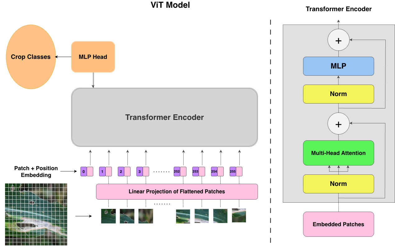
This token sequence is then processed through an encoder that has a depth of six layers and four attention heads. Each encoder layer contains Multi-Head Self-Attention to compute the global relationships between the patches. Each layer is also paired with a Multi-layer Perceptron (MLP) block that contains GELU activations, pre-layer normalization, and dropout to help stabilize training. Standard ViT architectures typically use much larger dimensions, such as the 768-dimensional embedding used in the original ViT model⁸. However, vision transformers do not have the inductive biases of convolutional models which causes them to have lower accuracies when trained on limited datasets²⁶. It has also been demonstrated that larger transformer networks inherently struggle under limited data conditions²⁷. Due to these limitations with our restricted dataset, we purposefully downsized the model to a hidden dimension of 256 along with lower layer and head counts. These changes follow the design principles outlined in recent data-efficient transformer literature.

The final classification head takes the transformed CLS token and converts it into logits across the 13 classes. This is also optimized with cross-entropy loss and the AdamW optimizer. 

A major architectural challenge highlighted by the foundational ViT literature is that ViTs lack the translational invariance and spatial locality of CNNs⁸. Due to this, ViTs usually require pre-training on massive datasets, such as ImageNet-21k²⁸, in order to achieve competitive performances with CNNs. In our study, the ViT model was trained completely from scratch with a dataset of around 16,000 images. Training our model from scratch on a constrained dataset like this can limit its ability to fully converge to top performances. This means that this specific architecture is not intended to compete with the top modern standards, but rather serves an important purpose in our experiment. It acts as a controlled benchmark in studying how self-attention mechanisms perform under limited data circumstances when compared to CNNs and other traditional models under the same training conditions.

Results

The metrics across our 5-fold stratified cross-validation demonstrate that a model’s classification accuracy depends heavily on its architectural strengths rather than simply parameter size. Table 5 summarizes macro and weighted metrics along with the total parameters and inference speeds for each of our models. 

Model Architecture	Macro F1​-Score (%)	Weighted F1​-Score (%)	Macro Precision (%)	Macro Recall (%)	Total Parameters	Avg. CPU Inference Speed (ms/img)
Logistic Regression	30.31%	30.88%	35.97%	42.40%	159,757	0.04
Neural Network	59.62%	61.39%	58.20%	64.06%	13,936,141	10.23
Convolutional Neural Network	89.40%	89.68%	88.32%	91.26%	3,702,541	47.29
Vision Transformer	88.26%	88.92%	89.26%	88.79%	3,219,853	89.19

The logistic regression model set the performance floor as it finished with a low weighted F1-score of 30.88% and a macro F1-score of 30.31% (Table 5). The deep Neural Network showed solid improvement, achieving 61.39% weighted F1-score and 59.62% macro F1-score (Table 5). This gap in performance shows that adding deep hidden layers and ReLU activations allows the model to learn non-linear patterns. However, flattening these pixels into a single vector limits the model’s ability to understand the spatial context that is needed to classify crop diseases.

Our more complex models in the CNN and ViT performed significantly better than the simpler logistic regression and neural network models. These two models also achieved very similar results. Our CNN had the highest overall performance with a weighted F1-score of 89.68% and a macro F1-score of 89.40% (Table 5). The ViT also performed competitively, yet slightly behind the CNN with an 88.92% weighted F1-score and an 88.26% macro F1-score (Table 5). A paired t-test on the macro F1-scores across the cross-validation folds also confirmed that the small 1.14% performance gap between the CNN and ViT is statistically significant (p < 0.05) even though they had very similar performances.

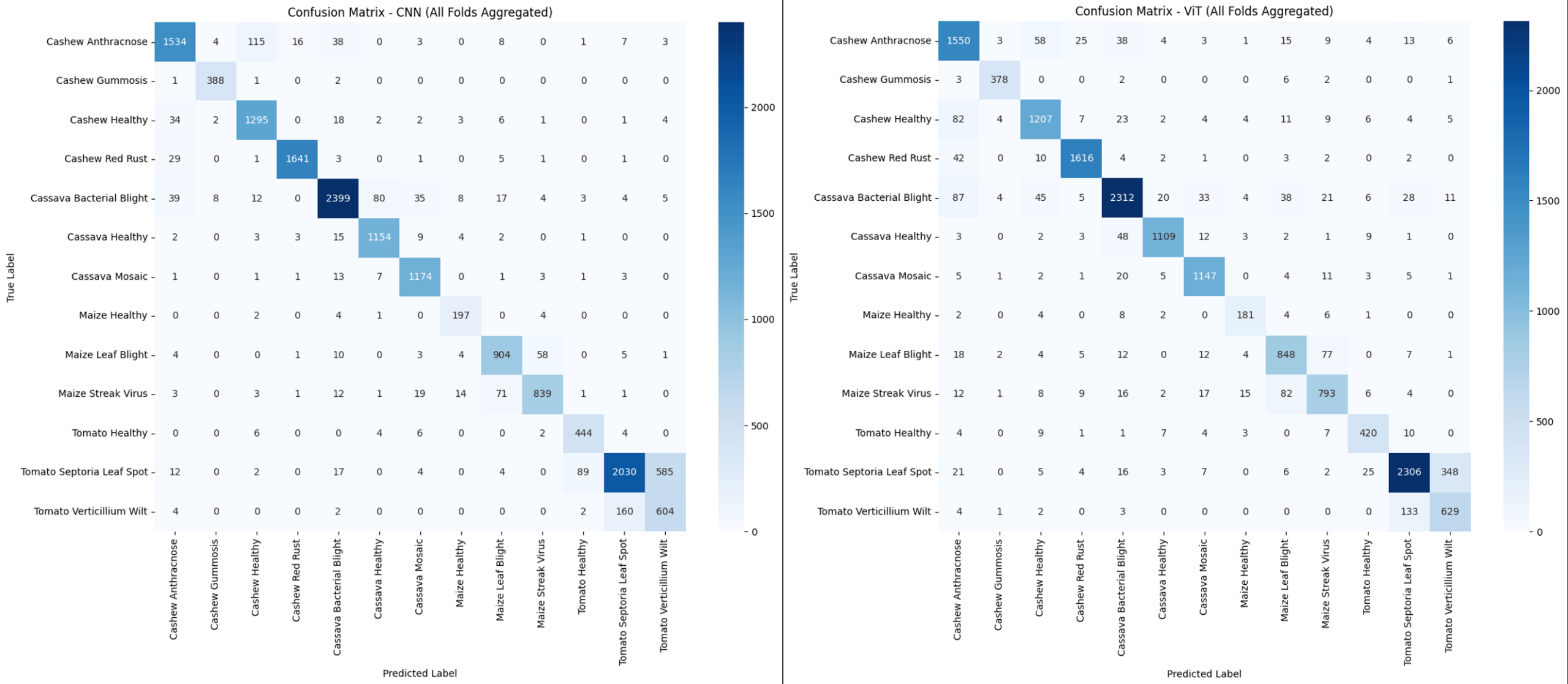
Our comparison between the macro-averaged metrics and the weighted averages shows how severely the class imbalances in the dataset impacted model training. Looking at the confusion matrices (Figure 3), our Logistic Regression and Neural Network models developed strong biases toward the heavily represented majority classes. Specifically, 1,349 true Tomato Septoria Leaf Spot instances were misclassified as Tomato Verticillium Wilt. There were also 551 true Cassava Mosaic samples that were incorrectly classified as Maize Healthy. The Neural Network lessened these distribution errors but still demonstrated issues when dealing with similar leaves. For example, it incorrectly predicted 729 true Tomato Septoria Leaf Spot samples as Tomato Verticillium Wilt.

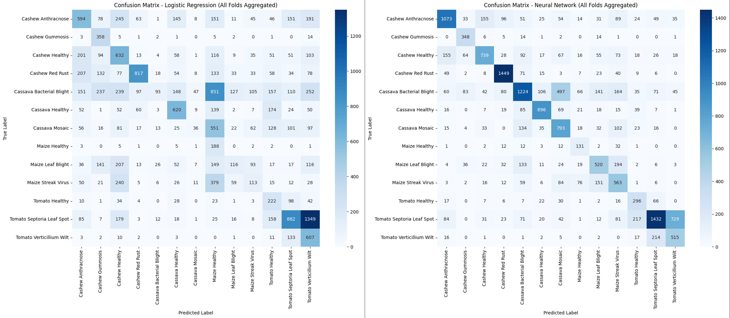
The CNN and ViT architectures reduced this imbalance better because of their specialization for image classification. However, they still struggled with differentiating visual similarities between certain leaves. For the CNN, Tomato Verticillium Wilt was very problematic as 160 out of 772 true Tomato Verticillium Wilt samples were misclassified as Tomato Septoria Leaf Spot (Figure 4). This pattern suggests that local convolutional filters struggle to tell the difference between smaller leaf spots and broader wilting. Our ViT architecture (Figure 4) on the other hand showed an opposite error pattern. Using global self-attention, the ViT was able to achieve higher distinctions for the wilt class as it only misclassified 133 samples as Septoria Leaf Spot. This represents a 16.88% reduction in this specific error compared to the CNN. However, the ViT also showed a reduced performance in macro-precision for Septoria Leaf Spot as it had 348 total false positive predictions within that category. This shows how ViTs are effective in understanding larger leaf changes but struggle with more precise details, especially when trained from scratch on mid-sized datasets.

We also tracked the training and validation trajectories for loss and accuracy across all epochs (Figures 5 and 6) to evaluate the optimization and stability of each model.

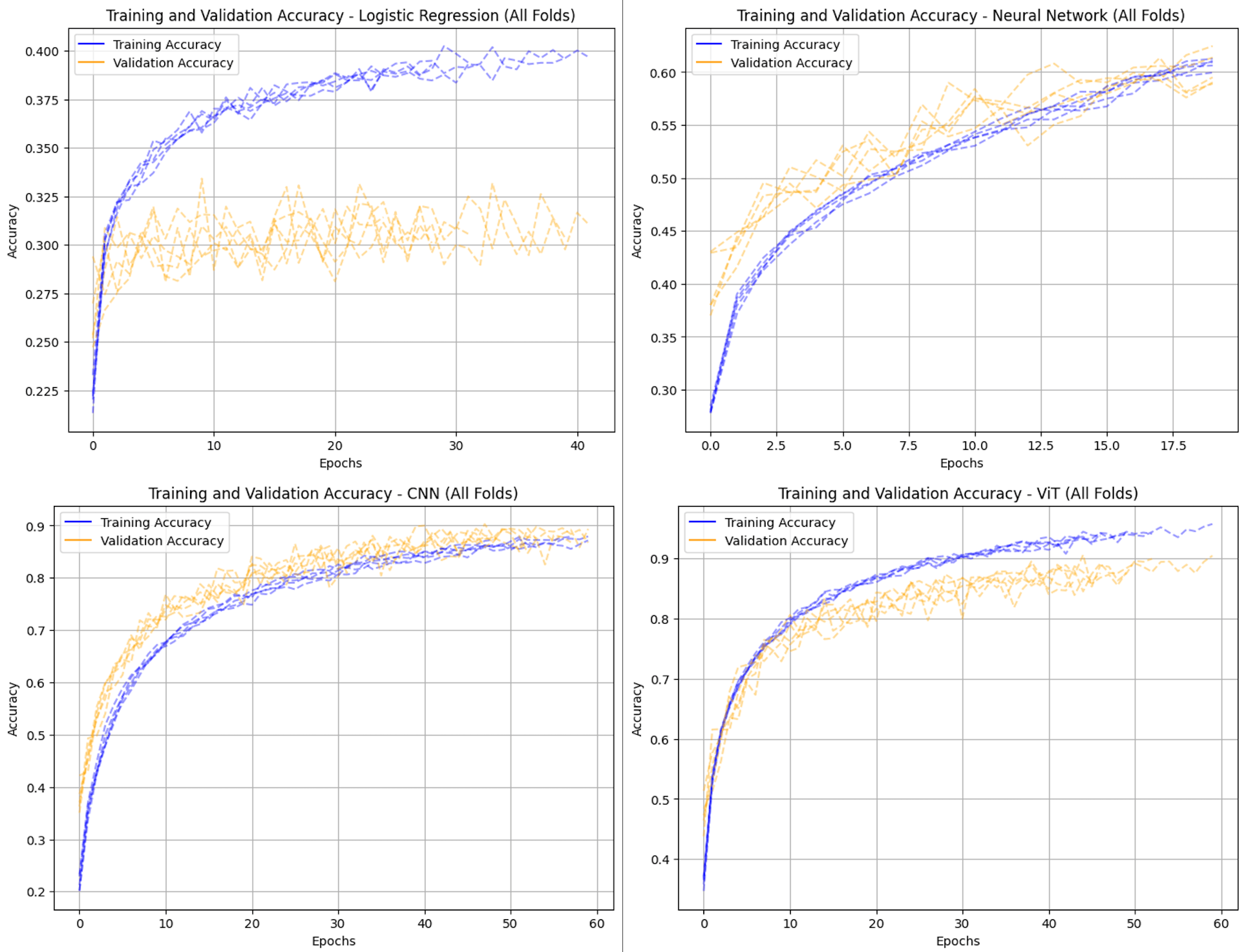
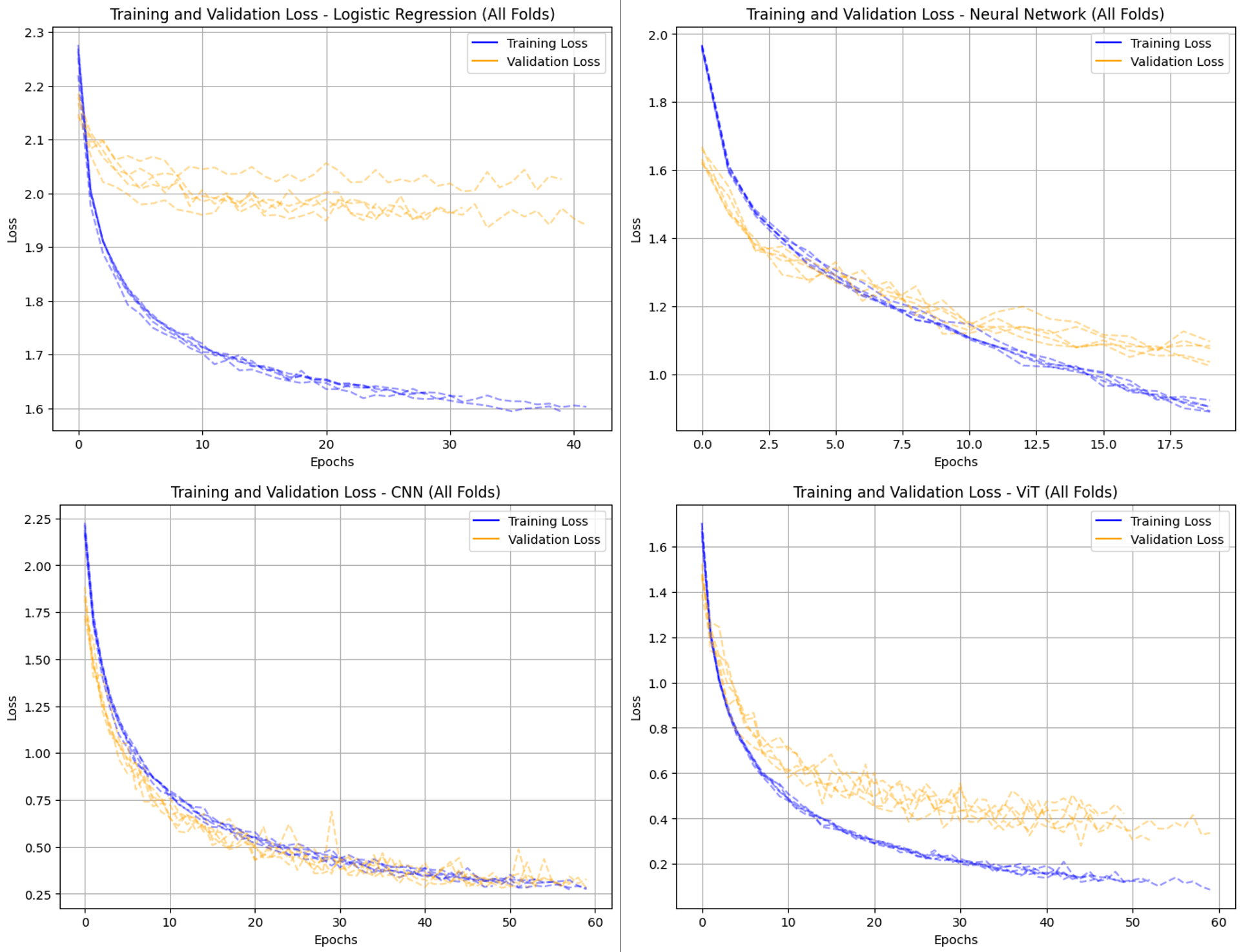
Our Logistic Regression model reached an early flatline as the training loss and accuracy graphs completely stalled within 5 epochs. The unstable validation folds and how the model struggled to stabilize suggests that it was grossly underfitting. This reflects how these simple models lack the ability to handle a 13-class crop disease distribution. The Neural Network model maintained steady convergence between its training and validation paths. However, it faced a clear limit around epoch 15. This suggests that its dense layers can decrease overfitting, but struggle with accuracy because they do not have any spatial context for classifying images. 

The optimization trends for the CNN and ViT clearly display their structural differences. The CNN converged very smoothly for all 5 independent folds and its validation curves closely matched the training curves as it reached steady optimization by epoch 60. This underscores how reliable convolutional layers are in stabilizing training. In contrast, the ViT displayed a clear learning lag during the first 15 epochs as shown by its slow decay in validation loss. The ViT validation paths also oscillate throughout the run, exposing the optimization instability of self-attention mechanisms when learning spatial relationships from scratch on limited data. This also directly explains why the ViT’s final macro performance is slightly below the localized CNN.

We measured parameter counts and inference speeds for each architecture (Table 5) to gauge their practicality for low-cost devices in developing regions. While the Logistic Regression model has the smallest computational footprint at 159,757 parameters, its poor performance makes it functionally unusable. The Neural Network required a large 13,936,141 parameters because every input pixel maps to a dense linear connection. Due to this, the model requires a very large memory footprint while also giving poor classification results. These models also exhibited low average CPU inference speeds of 0.04 ms and 10.23 ms for the Logistic Regression and Neural Network models respectively. However, their low classification performances make these fast processing speeds impractical for actual field deployment.  

The parameter counts and inference speeds for our CNN and the Vision Transformer models show their distinct trade-offs for deployment. The CNN achieved the highest accuracy while also having an efficient parameter count of 3,702,541 and an inference latency of 47.29 ms per image. This suggests that our CNN is highly suitable for low-cost mobile use. In comparison, our custom Vision Transformer was very comparable in size as it required a slightly lower footprint of 3,219,853 parameters. However, despite having fewer parameters, the dense matrix operations needed for multi-head self-attention led to a significant decrease in inference speeds for the ViT at 89.19 ms per image. This image processing delay along with its volatile optimization highlights that while transformers can match CNN’s accuracy on mid-sized datasets, CNNs still seem to remain the optimal choice for classification on fast, resource-limited devices.

Discussion

The 1.14% performance difference between our CNN at 89.68% weighted F1 and our ViT at 88.92% weighted F1 illustrates how architectural design impacts the performance of these models when trained on mid-sized datasets. The CNN’s higher overall metrics highlight the advantage they have due to their built-in spatial biases. Their sliding kernels allow the CNN to better understand leaf structures and more local, detailed textures. Their design also allows them to be very effective without needing extremely large datasets to learn basic shapes. In contrast, the ViT has no built-in understanding of spatial recognition in images. Because ViTs think of images as split up patches, they need to learn spatial relationships purely from scratch. Our ViT getting a weighted F1-score of 88.92 also proves that our hyperparameter optimization of shrinking the embedding dimension to 256 and using 4 attention heads successfully curbed any massive overfitting. However, the ViT validation loss curve’s wild oscillations confirm its sensitivity during optimization. Additionally, without large-scale pre-training, a from scratch-trained ViT struggles to fully stabilize on a limited dataset which explains its slight difference in performance compared to the CNN. 

Looking at the confusion matrices for our CNN and ViT highlights the clear trade-offs between their attributes and structures. Our CNN’s main weakness was confusing Tomato Verticillium Wilt for Tomato Septoria Leaf Spot. This mistake commonly occurred because of its localized filters that usually prioritize local pixel textures and fine edge differences. This means that the CNN’s limited field of view struggled to capture the larger structural variations of the leaf wilting or drooping caused by Verticillium Wilt. On the other hand, our ViT reduced this specific error by 16.88% and showed a clear advantage in understanding more global changes in the leaves. By calculating global self-attention across all non-overlapping patches at the same time, the ViT is able to understand the overall shape of the leaf. However, this focus on the entire image also led the ViT to lose some of its precision on Septoria Leaf Spot by incorrectly categorizing 348 wilt samples within that category. This indicates that it lacks the CNN’s finer precision for repeated, localized textures. This finding shows that the two models have clear complementary strengths which suggests that future agricultural frameworks could benefit significantly from hybrid CNN-ViT architectures that can utilize both localized and global features together.

Another important factor in evaluating these findings is the ecological validity of our dataset. The 16,323-image dataset we used in this study blends isolated leaves on clean backgrounds under stable lighting and true in-field agricultural images. This combination helps our models learn more basic disease characteristics while also training them on real-world variables like varying lighting, shadows, and chaotic backgrounds. However, because a major portion of the dataset uses clear, isolated leaves, the accuracy metrics in Table 5 likely represent an upper bound in performance. In actual real-world use, background noise might confuse local convolutional filters, while global self-attention mechanisms can get distracted by different scenery. While including in-field data helps support the real-world relevance of our findings, it is still a very important next step to validate these architectures on a 100% untouched, field dataset before these systems can be reliably used.

The computational efficiency of our models is just as important as their performance metrics for true in-field practicality. The CNN stands out as the most viable architecture for low-cost mobile devices in developing regions. It achieved the highest accuracies while also only requiring 3.7 million parameters, saving storage space and allowing for fast, real-time inference speeds. Our Vision Transformer on the other hand presents a more complex trade-off. Through our downscaling, the ViT had a final parameter footprint of 3,219,853 parameters, which is less than the CNN’s footprint. This disproves the assumption that transformers are too large for mobile storage. However, parameter counts do not directly correlate to the classification speed. The many matrix operations that are required for multi-head self-attention for every image patch causes a large computational requirement which slows its inference speeds. Overall, the CNN offers more consistent and immediate results, while the ViT’s increased processing time may limit its real-time usability. Therefore, while downscaled transformers can be very capable in terms of classification accuracy, CNNs are still the more optimal and dependable choice for resource-limited use.

Conclusion

Our study benchmarks the performance and computational requirements between classical, convolutional, and transformer-based crop disease architectures. Our results counter the common assumption that greater structural complexity automatically results in higher accuracies in data-restricted environments. Instead, our study shows that localized spatial inductive biases have a significant advantage over global self-attention mechanisms when training architectures from scratch on a medium-scale dataset. The CNN model achieved the highest overall classification accuracy with a macro-recall of 91.26% and a weighted F1-score of 89.68%. It also only needed an efficient footprint of 3,702,541 parameters. Our downscaled Vision Transformer on the other hand was capable of understanding broad structural changes, but its volatile validation loss oscillations highlight its optimization sensitivity caused by a lack of massive training data. The Logistic Regression and Neural Network architectures also clearly confirmed that the models lacking inherent spatial context struggle to handle image-based disease classification. Overall, the CNN was the strongest practical choice for real-world use among the models we evaluated for resource-constrained regions.

To build on these findings, future research should focus on two main steps to improve the ecological and practical utility of our image classification tools. First, the models in this study should be validated on untouched images from fields. This is necessary in order to test their performance in varying environments such as chaotic backgrounds, shifting light, and harsh shadows. Second, future research should utilize transfer learning with architectures pre-trained on massive image datasets. Specifically, architectures such as ResNet50²⁹ can give important architectural baselines that will help stabilize optimization and reduce the performance ceiling that these complex networks face. Additionally, using efficient transformer frameworks like DeiT-Small³⁰ that introduce a specialized distillation token which allows the multi-head self-attention mechanisms of ViTs to gain strong inductive biases from a teacher network. These specific frameworks will help stabilize training, handle class imbalances, and increase classification capabilities further than the limits of our scratch-trained models.

Acknowledgements

I would like to thank my mentor, Erick Siavichay, for his guidance and support throughout my research. His mentorship really deepened my knowledge of machine learning and further inspired my desire to learn more in the field.

References

1. Food and Agriculture Organization (FAO). Climate change fans spread of pests and threatens plants and crops, new FAO study. FAO Newsroom. 2021, https://www.fao.org/newsroom/detail/Climate-change-fans-spread-of-pests-and-threatens-plants-and-crops-new-FAO-study/en. [↩]
2. S. A. Miller, F. D. Beed, C. L. Harmon. Plant disease diagnostic capabilities and networks. Annual Review of Phytopathology. Vol. 47, pg. 15–38, 2009, https://doi.org/10.1146/annurev-phyto-080508-081743. [↩]
3. S. P. Mohanty, D. P. Hughes, M. Salathé. Using deep learning for image-based plant disease detection. Frontiers in Plant Science. Vol. 7, pg. 1419, 2016, https://doi.org/10.3389/fpls.2016.01419. [↩]
4. M. H. Saleem, J. Potgieter, K. M. Arif. Plant disease classification: a comparative evaluation of convolutional neural networks and deep learning optimizers. Plants. Vol. 9, no. 10, pg. 1319, 2020, https://doi.org/10.3390/plants9101319. [↩] [↩]
5. M. Tan, Q. V. Le. EfficientNet: Rethinking model scaling for convolutional neural networks. Proceedings of the 36th International Conference on Machine Learning (ICML). Vol. 97, pg. 6105–6114, 2019, https://proceedings.mlr.press/v97/tan19a.html. [↩]
6. Z. Liu, H. Mao, C.-Y. Wu, C. Feichtenhofer, T. Darrell, S. Xie. A ConvNet for the 2020s. Proceedings of the IEEE/CVF Conference on Computer Vision and Pattern Recognition (CVPR). pg. 11976–11986, 2022, https://openaccess.thecvf.com/content/CVPR2022/papers/Liu_A_ConvNet_for_the_2020s_CVPR_2022_paper.pdf. [↩]
7. B. Yang, M. Li, F. Li, H. Lu, M. Du, K. Zhao, M. Zheng, J. Cao. A novel plant type, leaf disease and severity identification framework using CNN and transformer with multi-label method. Scientific Reports. Vol. 14, pg. 11664, 2024, https://doi.org/10.1038/s41598-024-62452-x. [↩]
8. A. Dosovitskiy, L. Beyer, A. Kolesnikov, D. Weissenborn, X. Zhai, T. Unterthiner, M. Dehghani, M. Minderer, G. Heigold, S. Gelly, J. Uszkoreit, N. Houlsby. An image is worth 16×16 words: transformers for image recognition at scale. International Conference on Learning Representations (ICLR). 2021, https://openreview.net/pdf?id=YicbFdNTTy. [↩] [↩] [↩] [↩]
9. S. Mehdipour, S. A. Mirroshandel, S. A. Tabatabaei. A novel lightweight hybrid CNN–ViT for maize leaf disease classification. Scientific Reports. Vol. 16, pg. 10468, 2026, https://doi.org/10.1038/s41598-026-41190-2. [↩]
10. R. Karthik, A. Ajay, A. Singh Bisht, T. Illakiya, K. Suganthi. A deep learning approach for crop disease and pest classification using swin transformer and dual-attention multi-scale fusion network. IEEE Access. Vol. 12, pg. 152639–152655, 2024, https://doi.org/10.1109/ACCESS.2024.3481675. [↩] [↩]
11. G. Shandilya, S. Gupta, H. G. Mohamed, S. Bharany, A. U. Rehman, S. Hussen. Enhanced maize leaf disease detection and classification using an integrated CNN-ViT model. Food Science & Nutrition. Vol. 13, no. 7, pg. e70513, 2025, https://doi.org/10.1002/fsn3.70513. [↩] [↩]
12. A. A. Paul, S. M. Tawhid, A. K. Mohim, D. Nandi. Explainable hybrid CNN-transformer framework for papaya leaf disease classification with layer-wise grad-cam analysis. AIUB Journal of Science and Engineering. Vol. 24, no. 2, 2026, https://doi.org/10.53799/vxkj7t08. [↩] [↩]
13. M. Sandler, A. Howard, M. Zhu, A. Zhmoginov, L. Chieh Chen. MobileNetV2: inverted residuals and linear bottlenecks. Proceedings of the IEEE Conference on Computer Vision and Pattern Recognition (CVPR). pg. 4510–4520, 2018, https://openaccess.thecvf.com/content_cvpr_2018/papers/Sandler_MobileNetV2_Inverted_Residuals_CVPR_2018_paper.pdf. [↩]
14. R. Sharma, A. Singh, Kavita, N. Z. Jhanjhi, M. Masud, E. S. Jaha, S. Verma. Plant disease diagnosis and image classification using deep learning. Computers, Materials & Continua. Vol. 71, no. 2, pg. 2125–2140, 2022, https://doi.org/10.32604/cmc.2022.020017. [↩]
15. M. T. Ahad, Y. Li, B. Song, T. Bhuiyan. Comparison of CNN-based deep learning architectures for rice diseases classification. Artificial Intelligence in Agriculture. Vol. 9, pg. 22–35, 2023, https://doi.org/10.1016/j.aiia.2023.07.001. [↩]
16. G. Batchuluun, S. H. Nam, K. R. Park. Deep learning-based plant classification and crop disease classification by thermal camera. Journal of King Saud University – Computer and Information Sciences. Vol. 34, no. 10, pt. B, pg. 10474–10486, 2022, https://doi.org/10.1016/j.jksuci.2022.11.003. [↩]
17. G. Sachdeva, P. Singh, P. Kaur. Plant leaf disease classification using deep Convolutional neural network with Bayesian learning. Materials Today: Proceedings. Vol. 45, pt. 6, pg. 5527–5532, 2021, https://doi.org/10.1016/j.matpr.2021.02.312. [↩]
18. U. K. Lilhore, A. L. Imoize, C.-C. Lee, S. Simaiya, S. K. Pani, N. Goyal, A. Kumar, C.-T. Li. Enhanced convolutional neural network model for cassava leaf disease identification and classification. Mathematics. Vol. 10, no. 4, pg. 580, 2022, https://doi.org/10.3390/math10040580. [↩]
19. M. Timothy, O. John, A. Aibinu, B. Adebisi. Detection and classification system for cashew plant diseases using convolutional neural network. Proceedings of the 5th International Conference on Future Networks and Distributed Systems (ICFNDS). pg. 225–232, 2022, https://doi.org/10.1145/3508072.3508107. [↩]
20. S. Srinivasan, R. A, N. B. A, V. P. G, V. R. S. Multi-class classification of plant leaf diseases using a hybrid deep neural transformer system and explainable AI techniques. Scientific Reports. Vol. 16, pg. 18161, 2026, https://doi.org/10.1038/s41598-026-48103-3. [↩]
21. M. N. Noor, M. Masab, F. Haneef, M. Hussain, M. Yaqoob, T. Mazhar, M. A. Khan, G. Aldehim. An effective approach for recognition of crop diseases using advanced image processing and YOLOv8. Food Science & Nutrition. Vol. 14, no. 2, pg. e71504, 2026, https://doi.org/10.1002/fsn3.71504. [↩]
22. P. M. Kwabena, V. Akoto-Adjepong, K. Adu, M. A. Ayidzoe, E. A. Bediako, O. Nyarko-Boateng, S. Boateng, E. F. Donkor, F. U. Bawah, N. S. Awarayi, P. Nimbe, I. K. Nti, M. Abdulai, R. R. Adjei, M. Opoku. Dataset for Crop Pest and Disease Detection. Mendeley Data. Version 1, 2023, https://doi.org/10.17632/bwh3zbpkpv.1. [↩]
23. M. S. Krishna, P. Machado, R. I. Otuka, S. W. Yahaya, F. N. dos Santos, I. K. Ihianle. Plant leaf disease detection using deep learning: a multi-dataset approach. J. Vol. 8, no. 1, pg. 4, 2025, https://doi.org/10.3390/j8010004. [↩]
24. I. Loshchilov, F. Hutter. Decoupled weight decay regularization. International Conference on Learning Representations (ICLR). 2019, https://openreview.net/pdf?id=Bkg6RiCqY7. [↩]
25. J. Huang, Y. Wang, M. Wang. Class-adaptive weighted broad learning system with hybrid memory retention for online imbalanced classification. Electronics. Vol. 14, no. 17, pg. 3562, 2025, https://doi.org/10.3390/electronics14173562. [↩]
26. Z. Lu, H. Xie, C. Liu, Y. Zhang. Bridging the gap between vision transformers and convolutional neural networks on small datasets. Advances in Neural Information Processing Systems (NeurIPS). Vol. 35, pg. 14352–14365, 2022, https://proceedings.neurips.cc/paper_files/paper/2022/file/5e0b46975d1bfe6030b1687b0ada1b85-Paper-Conference.pdf. [↩]
27. Y. Liu, E. Sangineto, W. Bi, N. Sebe, B. Lepri, M. De Nadai. Efficient training of visual transformers with small datasets. Advances in Neural Information Processing Systems (NeurIPS). Vol. 34, pg. 23818–23830, 2021, https://proceedings.neurips.cc/paper_files/paper/2021/file/c81e155d85dae5430a8cee6f2242e82c-Paper.pdf. [↩]
28. T. Ridnik, E. Ben-Baruch, A. Noy, L. Zelnik-Manor. ImageNet-21K pretraining for the masses. Advances in Neural Information Processing Systems (NeurIPS). Vol. 34, pg. 23831–23842, 2021, https://openreview.net/pdf?id=Zkj_VcZ6ol. [↩]
29. K. He, X. Zhang, S. Ren, J. Sun. Deep residual learning for image recognition. Proceedings of the IEEE Conference on Computer Vision and Pattern Recognition (CVPR). pg. 770–778, 2016, https://openaccess.thecvf.com/content_cvpr_2016/papers/He_Deep_Residual_Learning_CVPR_2016_paper.pdf. [↩]
30. H. Touvron, M. Cord, M. Douze, F. Massa, A. Sablayrolles, H. Jégou. Training data-efficient image transformers & distillation through attention. Proceedings of the International Conference on Machine Learning (ICML). PMLR 139, pg. 10347–10357, 2021, https://proceedings.mlr.press/v139/touvron21a/touvron21a.pdf. [↩]