Robustness of AI-Based Environmental Sound Recognition Under Controlled Gaussian Noise

Abstract

Although deep learning-based environmental sound recognition (ESR) systems achieve strong performance under controlled conditions, their robustness often degrades in real-world acoustic environments containing overlapping sounds, reverberation, and background noise. While augmentation-based robustness strategies are widely used, differences in datasets, preprocessing pipelines, feature extractors, model architectures, and evaluation protocols can make direct comparisons across studies difficult. This study compares additive noise, time shifting, and mixup augmentation strategies using a fixed transfer-learning pipeline based on pretrained YAMNet embeddings and the ESC-50 dataset. Models were evaluated under both clean and noisy acoustic conditions across multiple signal-to-noise ratio (SNR) levels. Experimental results across five repeated stratified splits showed that additive Gaussian-noise augmentation substantially improved robustness under noisy evaluation conditions. At 0 dB SNR, mean accuracy increased from 10.75 ± 1.68% for the clean baseline to 57.70 ± 4.16% for the noise-augmented model. Significant improvements were observed at every noisy SNR level from 20 to 0 dB, and all five improvements remained statistically significant after Holm correction across the 18 model-by-condition comparisons. Time shifting did not significantly improve noisy-condition accuracy. Mixup showed higher mean clean-condition accuracy than the baseline, but this difference was not statistically significant after Holm correction, and mixup did not improve performance under noisy evaluation conditions. Overall, the findings provide empirical guidance for selecting augmentation strategies for environmental sound recognition systems operating under controlled Gaussian-noise conditions.

keywords: Environmental sound recognition, data augmentation, robustness, deep learning, audio classification

Introduction

Environmental Sound Recognition (ESR) can be described as a sound recognition technique where non-speech sounds such as alarm sounds, sirens, steps, rain sounds, engine sounds, and household sounds are classified automatically.  Environmental sound recognition does not benefit from linguistic units or phoneme sequences. These properties are fundamental to speech recognition systems. Instead, environmental sounds exhibit high intra-class variability and non-rhythmic temporal structure. They also show broad spectral variation, which makes robust classification challenging^1,2.

In real-world environments, target sounds rarely occur in isolation. They are mixed with background noise, competing sound sources, reverberation, and recording-device distortions. Although modern environmental sound recognition systems achieve strong performance on benchmark datasets, their accuracy often decreases substantially when evaluated under degraded acoustic conditions^1,2. There have been many proposed techniques to enhance robustness through data augmentation that include additive noise, time shifts, mixup, and spectrogram augmentations like SpecAugment^3,4,5. These augmentation techniques are often compared on datasets that are different from each other, use different preprocessing pipelines, features, models, etc., which makes it hard to distinguish the impact of the augmentation itself from the other factors of the experiments. Consequently, there remains a need for controlled comparisons in which augmentation methods are evaluated under the same transfer-learning pipeline, feature representation, and noisy evaluation protocol.

Improvements in deep learning methods and transfer learning have greatly impacted the performance of ESR on standard databases. Recent studies have further demonstrated that large-scale audio pretraining and transfer learning significantly improve environmental sound classification performance, particularly when labeled training data are limited^6,7. The use of pretrained models, such as YAMNet, relying on large datasets such as AudioSet, leads to high-quality embeddings with good generalization capabilities over different tasks^8,9. However, this is not a sufficient factor in ensuring robustness if the classifiers are trained on limited or narrowly distributed training data. As a result, robustness-oriented training strategies are increasingly necessary.

This study investigates how additive Gaussian noise, time shifting, and mixup influence the robustness of a transfer-learning-based environmental sound recognition system when all augmentation strategies are evaluated under the same pretrained embedding pipeline and controlled noisy evaluation conditions.

This study does not propose a new augmentation algorithm. Instead, it provides a controlled comparison of commonly used augmentation strategies under the same environmental sound recognition pipeline. By keeping the dataset, embedding extractor, preprocessing procedure, and evaluation structure consistent, this study enables a controlled comparison of the effects of each augmentation strategy on robustness under noisy acoustic conditions.

The main contributions of this study are:

• A controlled comparison of additive noise, time shifting, and mixup augmentation strategies under a fixed YAMNet-based environmental sound recognition pipeline.
• An evaluation of environmental sound recognition robustness across multiple signal-to-noise ratio conditions, enabling systematic analysis of performance degradation under increasing background noise.
• Empirical evidence that additive noise augmentation provides stronger low-SNR robustness than time shifting and mixup under the tested conditions.

Background and Technical Foundations

Contemporary ESR systems rely on time-frequency representations such as log mel spectrograms. These representations enable the examination of local structures, which can be effectively leveraged within CNN architectures for time-based audio analysis⁸. Pre-training has also been shown to be highly effective in learning generalized audio features. According to Hershey et al., features obtained through AudioSet pre-training are sufficiently general to perform well across a range of audio applications, including environmental sound classification⁸.

YAMNet provides 1024-dimensional embeddings learned from a deep convolutional network trained on millions of labeled audio examples¹⁰. Recent advances in self-supervised and representation-learning approaches have further demonstrated the effectiveness of learned audio embeddings for downstream acoustic classification tasks¹¹. Despite the benefits of pretrained representations, classifiers can still experience substantial performance degradation when training and evaluation conditions differ^12,13.

Background noise influences the statistical properties of spectrograms by masking important spectral information and introducing additional spectral energy. The measure commonly used to determine levels of background noise is signal-to-noise ratio (SNR)¹⁴. Models trained on clean spectrograms overemphasize small spectral details that are not robust under noisy conditions. Prior work has shown that deep neural networks trained under mismatched acoustic conditions can experience significant performance degradation, highlighting the importance of robustness-oriented training strategies^12,13. As the signal-to-noise ratio decreases, model performance significantly deteriorates. This observation is in line with the issue of distribution shift, whereby models developed under one data distribution exhibit reduced performance when evaluated under different environmental conditions¹⁵.

Robustness to naturally occurring noise is related to, but distinct from, several broader approaches to model reliability. Domain adaptation attempts to reduce differences between source and target data distributions by learning features that remain useful across domains¹⁶. Adversarial robustness focuses on resistance to deliberately designed perturbations that cause incorrect predictions, rather than the random Gaussian corruption evaluated in this study¹⁷. Uncertainty quantification provides another complementary approach by estimating how confident a model should be in its predictions, which can help identify unreliable outputs under unfamiliar or degraded conditions¹⁸. These methods have not been applied in this study, but they provide promising paths to further the research in environmental sound recognition beyond augmentation-based robustness.

Related Work

Early work showed that incorporating acoustic-context information can improve sound-event detection compared with context-independent approaches¹⁹.

With the arrival of deep learning, it was possible for ESR to move towards a more data-driven approach to the learning of features. Performance improved with the use of convolutional neural networks, although environmental sound classifiers could still be sensitive to changes in acoustic conditions. Salamon and Bello showed that audio data augmentation can improve environmental sound classification and that the effects of individual augmentation methods vary across sound classes³. Earlier CNN-based environmental sound classification studies also demonstrated that deep neural networks could outperform traditional handcrafted feature approaches, helping establish the foundation for modern ESR systems^20,21. The more recent work in the field of environmental sound classification has involved the use of transfer learning and pre-trained audio features, allowing for significant gains compared to training from scratch^6,7,22.

In relation to the recognition of speech, Ko et al.¹⁴ showed that noise-aware training of a model can lower the word error rate by introducing realistic distortion during the training process. SpecAugment applies augmentation directly to log-mel spectrograms by masking selected time intervals and frequency bands, encouraging the model to rely less on any single local feature⁵. Unlike the waveform- and embedding-level strategies evaluated in this study, SpecAugment modifies the time-frequency representation itself. It was not included in the present comparison because the experimental pipeline used fixed pretrained YAMNet embeddings rather than training directly on spectrogram inputs. Broader machine learning research has similarly shown that augmentation techniques improve model generalization by exposing models to a wider range of input variations during training^23,24. Although speech and environmental sounds differ substantially in their signal characteristics, both domains have shown robustness improvements through augmentation-based training strategies. Time shifting preserves the class label while changing the temporal position of an event, encouraging temporal invariance³. Mixup generates augmented training examples by linearly combining pairs of samples and their corresponding labels⁴. Because these interpolated examples may not correspond to naturally occurring acoustic mixtures, their benefits may differ from those of direct noise augmentation.

Prior studies have demonstrated the effectiveness of augmentation techniques for improving robustness in ESR and speech recognition systems. However, differences in datasets, preprocessing methods, embedding extractors, and evaluation protocols make direct comparisons between augmentation strategies difficult. This study addresses that limitation by evaluating additive noise, time shifting, and mixup augmentation under a consistent ESR transfer-learning pipeline and shared evaluation setting.

To reduce differences introduced by datasets, architectures, preprocessing pipelines, and evaluation protocols, this study evaluates the augmentation strategies within a single controlled pipeline.

Methodology

Dataset

The ESC-50 dataset consists of 50 classes of environmental sounds, ranging from animals to natural sounds, human activity, and urban noise. Each class has 40 examples of audio files, making a total of 2000 labeled samples. The audio files are all 5 seconds long and are sampled at 44.1 kHz. The audio samples were recorded in real-world settings like streets, parks, homes, and public areas.

ESC-50 was selected because it provides 50 environmental sound classes with exactly 40 recordings per class, creating a balanced structure for repeated stratified comparisons¹. UrbanSound8K is also a widely used environmental sound dataset, but it focuses on 10 urban sound classes and contains an unequal number of recordings across classes². Because the objective of this study was to compare augmentation strategies under the same controlled pipeline rather than focus specifically on urban noise, ESC-50 offered broader sound-category coverage and a balanced class distribution. These properties made it easier to assign the same number of training, validation, and testing recordings from every class across the five repeated splits.

The experiments used five repeated stratified train, validation, and test splits with random seeds 11, 22, 33, 44, and 55. For each of the 50 classes, 28 recordings were assigned to training, 4 to validation, and 8 to testing, corresponding to 70%, 10%, and 20% of the data, respectively. This produced 1,400 training samples, 200 validation samples, and 400 testing samples in each repeated split. Model selection and early stopping were based only on validation performance, while the held-out test set was used for final evaluation. The official ESC-50 five-fold cross-validation protocol was not used, which is acknowledged as a limitation when comparing the results directly with studies that follow the official protocol.

For each repeated split, the corresponding seed (11, 22, 33, 44, or 55) was used once at the beginning of the split to initialize the Python, NumPy, and TensorFlow random number generators, making the sequence of data partitioning and subsequent training operations reproducible. The four classifier models were trained sequentially without resetting the global random-number generators before each model; therefore, their random weight initializations were reproducible within the experimental sequence but were not constrained to be identical across augmentation conditions.  For noise and time-shift augmentation, a sample-specific NumPy random generator was initialized using the seed  , where s is the repeated-split seed and  is the training-sample index. Mixup pairings were generated using a NumPy random generator initialized with the split seed. For evaluation noise, the random seed was calculated as  , where SNR is the evaluation signal-to-noise ratio in decibels and i is the test-sample index, and this value was used to initialize a NumPy random generator. This ensured that every model received the same corrupted waveform for a given split, sample, and SNR condition.

Training Configuration and Experimental Parameters

Component	Value
Noise source	Synthetic zero-mean Gaussian noise generated with NumPy
Training SNR levels	20, 15, 10, 5, and 0 dB
Feature Extractor	Frozen pretrained YAMNet embedding extractor
Embedding dimension	1024
Classification head	Dense (512) → BatchNorm → Dropout (0.4) → Dense (256) → BatchNorm → Dropout (0.3) → Softmax (50 classes)
Optimizer	Adam
Learning rate	0.001
Maximum epochs	30
Batch size	64
Early stopping	Patience 5; restore best weights
Split protocol	Five repeated stratified 70/10/20 train-validation-test splits
Random seeds	11, 22, 33, 44, and 55
Time shift	±1,600 samples (±0.1 s), zero-padded
Mixup	YAMNet embedding level, λ = 0.5

Each audio clip was resampled to 16 kHz and converted to mono, padded or truncated to a fixed duration of 5 seconds (80,000 samples), and peak-normalized by dividing the waveform by its maximum absolute sample value when that value was greater than zero.

For each 5-second clip, YAMNet produced a sequence of frame-level 1024-dimensional embeddings. These frame-level embeddings were averaged across the temporal dimension using mean pooling to obtain a single 1024-dimensional clip-level representation, which was then used as input to the classifier. The same temporal mean-pooling procedure was applied to all training and evaluation conditions. Using fixed pretrained embeddings ensures that differences in model performance can be more directly attributed to the augmentation strategies rather than changes in feature extraction. YAMNet was selected because it provides pretrained audio embeddings derived from large-scale AudioSet training, enabling consistent feature extraction across all augmentation conditions.

Augmentation Strategies

Four training models were evaluated in order to analyze the impact of data augmentation on model robustness:

• Clean baseline, with no augmentation
• Additive Gaussian noise, using synthetic zero-mean Gaussian noise generated with NumPy and scaled to signal-to-noise ratios of 20, 15, 10, 5, and 0 dB; no external environmental noise corpus was used.
• Time shifting,randomly shifting each waveform forward or backward by up to ±0.1 seconds (1,600 samples at 16 kHz), with uncovered samples filled with zeros rather than circularly wrapped.
• Mixup, combining pairs of YAMNet embeddings and their corresponding one-hot labels using a fixed mixing coefficient of λ⁴.

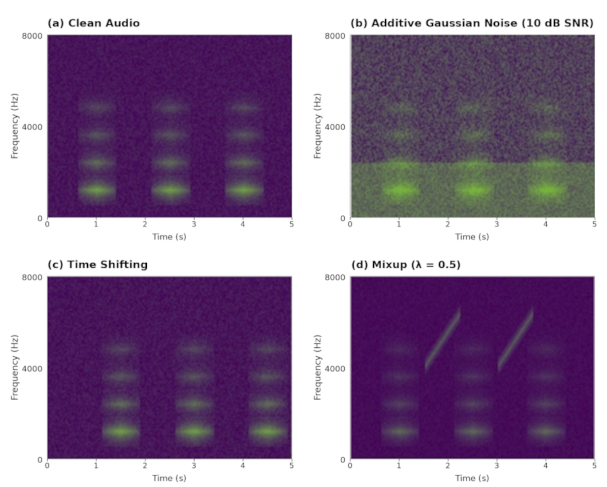
All augmentations were applied only during training. To ensure fair comparison, all trained models were evaluated on the same clean test set and the same noisy test sets across SNR levels.

For Gaussian-noise scaling, signal power was calculated from the amplitude-normalized waveform as the mean squared sample value, . For a target SNR in decibels, the linear SNR

was calculated as , and the target noise power was set to . Zero-mean Gaussian noise was then generated with standard deviation  and added directly to the waveform. A small constant of  was added to the signal-power calculation for numerical stability. No additional clipping was applied after noise addition. The same Gaussian-noise scaling procedure was used for both training augmentation and generation of the noisy evaluation sets.

Training Conditions and Model Variants

The experimental pipeline used a fixed pretrained YAMNet embedding extractor followed by a trainable neural network classification head. The YAMNet model was frozen, and only the classification head was trained. This design enabled a controlled comparison of augmentation strategies while keeping the feature extraction process consistent across conditions.

The classification head consisted of a dense layer with 512 units, batch normalization, dropout of 0.4, a second dense layer with 256 units, batch normalization, dropout of 0.3, and a final softmax output layer with 50 units corresponding to the ESC-50 classes. The clean, additive-noise, and time-shift models were trained using sparse categorical cross-entropy loss. Because mixup produced soft one-hot label combinations, the mixup model was trained using categorical cross-entropy loss. All models used the Adam optimizer with a learning rate of 0.001 and accuracy as the primary evaluation metric.

For each repeated split, four classification models were trained: one clean baseline, one additive-noise-augmented model, one time-shift-augmented model, and one mixup-augmented model. All four models used the same YAMNet embedding extractor, classification-head architecture, validation subset, and held-out test subset. The validation set remained unaugmented for all four training conditions and was used consistently for model selection and early stopping. For time-shift augmentation, audio clips were randomly shifted forward or backward by up to ±0.1 seconds (1,600 samples at a 16 kHz sampling rate), with uncovered samples filled with zeros. For additive noise augmentation, synthetic zero-mean Gaussian noise generated with NumPy was added to training samples at SNR levels of 20, 15, 10, 5, and 0 dB; no external environmental noise corpus was used. Mixup augmentation was applied at the YAMNet-embedding level by combining pairs of embeddings and their corresponding one-hot labels using a fixed mixing coefficient of . This structure allowed the performance of clean-trained and augmentation-trained models to be compared under matching test conditions.

Each model received 1,400 training examples per repeated split. For additive-noise training, one SNR level was selected uniformly at random from 20, 15, 10, 5, or 0 dB for each training clip, producing one noise-augmented version per original clip rather than copies at all five SNR levels. For time-shift training, each clip received one shift sampled uniformly at random from −1,600 to +1,600 samples, corresponding to −0.1 to +0.1 seconds at 16 kHz. For mixup, each clean embedding was paired with one shuffled embedding, producing one mixed example per original training example. These augmentations were generated once before model training and were not regenerated at every epoch. Clean examples were not additionally retained alongside the augmented examples for the augmentation-trained models. All four models therefore received the same number of training examples and used the same batch size and maximum number of epochs, although the actual number of optimization steps could differ across models because early stopping was based on validation performance. Across seeds 11, 22, 33, 44, and 55, the clean baseline trained for 16, 17, 10, 13, and 10 epochs, respectively; the noise-augmented model trained for 26, 19, 27, 27, and 30 epochs; the time-shift-augmented model trained for 11, 16, 12, 16, and 13 epochs; and the mixup-augmented model trained for 19, 21, 22, 18, and 19 epochs. With 1,400 training samples and a batch size of 64, each epoch contained 22 training updates, corresponding to 352, 374, 220, 286, and 220 updates for the clean baseline; 572, 418, 594, 594, and 660 for the noise-augmented model; 242, 352, 264, 352, and 286 for the time-shift-augmented model; and 418, 462, 484, 396, and 418 for the mixup-augmented model.

Models were trained for up to 30 epochs with a batch size of 64. Early stopping was used with a patience of 5 epochs, and the best model weights were restored based on validation accuracy. A reduce-on-plateau learning rate schedule was also used to lower the learning rate when validation loss stopped improving.

Evaluation Protocol

Models were evaluated on the same clean test set and on deterministic noisy test sets at 20, 15, 10, 5, and 0 dB SNR. Within each repeated split, every model received the same Gaussian-noise realization for each test sample and SNR level to ensure a controlled comparison. Accuracy was recorded separately for every seed and condition. Mean accuracy and sample standard deviation were calculated across the five repeated splits. Two-sided paired t-tests were used to compare each augmentation-trained model with the clean baseline at each evaluation condition. To account for the 18 model-by-condition comparisons, p-values were adjusted using the Holm procedure. Both unadjusted and Holm-adjusted p-values were examined, with statistical significance assessed at an adjusted p < .05.

Implementation Details

Experiments were implemented in Python using standard machine learning and audio processing libraries, including TensorFlow, Librosa²⁵, NumPy, and Scikit-learn. Audio preprocessing and feature extraction were performed using pretrained YAMNet embeddings. Training and evaluation were conducted under consistent preprocessing and augmentation settings across all experiments to ensure controlled comparison between augmentation strategies. All experiments were executed in a consistent local computing environment using the same software configuration for every repeated split.

To improve reproducibility, the overall implementation pipeline is summarized in Algorithm 1.

Algorithm 1. Experimental Pipeline

1. Load ESC-50 metadata and audio files.
2. For each random seed (11, 22, 33, 44, and 55), partition each class into 28 training samples, 4 validation samples, and 8 testing samples, producing repeated stratified 70/10/20 train-validation-test splits.
3. Encode class labels into numerical labels.
4. For each audio clip:
5. Resample audio to 16 kHz.
6. Convert to mono audio.
7. Pad or truncate to 5 seconds.
8. Peak-normalize each waveform by dividing by its maximum absolute sample value when nonzero.
9. For each training condition:

1. Extract clean YAMNet embeddings for the baseline and mixup conditions.
2. For additive-noise and time-shift conditions, augment each waveform before extracting its YAMNet embedding.
3. For mixup, combine pairs of clean YAMNet embeddings and their corresponding one-hot labels using λ = 0.5.
4. Train the neural network classification head using Adam optimization.

6. Evaluate all trained models on the same clean test set and deterministic Gaussian-noise test sets at 20, 15, 10, 5, and 0 dB SNR.
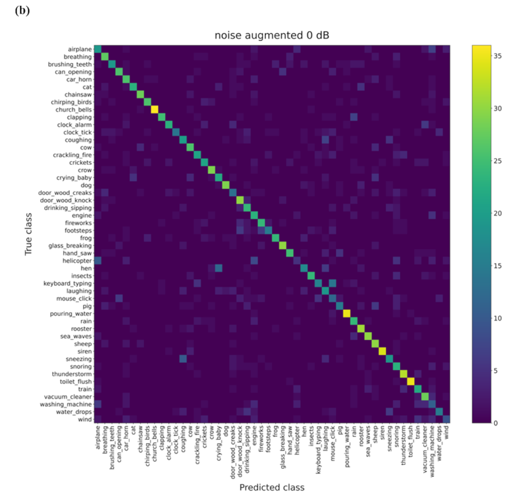
7. Record per-seed accuracy and generate confusion matrices for clean and 0 dB conditions.
8. Calculate mean accuracy and sample standard deviation across the five repeated splits, perform paired t-tests using the five split-level accuracies, and apply Holm correction across the 18 model-by-condition comparisons.

Results

This section presents the results obtained across five repeated stratified train, validation, and test splits. Clear differences in robustness were observed among the evaluated augmentation strategies under the shared Gaussian-noise SNR grid. Additive noise augmentation produced the strongest performance under every noisy evaluation condition. At 0 dB SNR, mean accuracy increased from 10.75 ± 1.68% for the clean baseline to 57.70 ± 4.16% for the noise-augmented model. This improvement remained statistically significant after Holm correction across the 18 model-by-condition comparisons (adjusted p = 0.0001978). Time shifting did not significantly improve noisy-condition accuracy, while mixup showed higher mean clean-condition accuracy than the baseline, but this difference was not statistically significant after Holm correction and did not produce significant gains under noisy evaluation conditions.

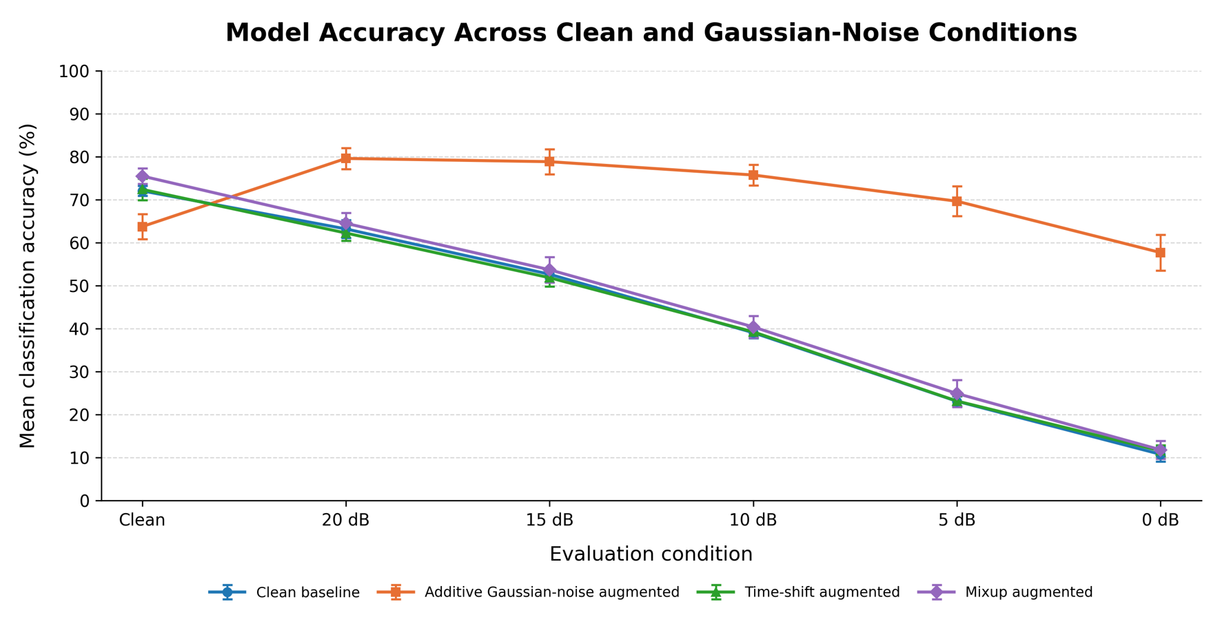
Figure 4 summarizes the mean accuracy trends across the clean and Gaussian-noise evaluation conditions, while Table 2 reports the corresponding mean accuracies and sample standard deviations. The clean baseline achieved a mean clean-condition accuracy of 72.05 ± 1.16%, but its performance declined steadily as the SNR decreased. Mean accuracy fell to 63.20 ± 2.06% at 20 dB, 52.65 ± 1.01% at 15 dB, 39.05 ± 1.27% at 10 dB, 23.10 ± 1.14% at 5 dB, and 10.75 ± 1.68% at 0 dB. These results demonstrate the substantial sensitivity of the clean-trained model to increasing Gaussian-noise severity.

The noise-augmented model demonstrated the strongest robustness across all noisy evaluation conditions. Mean accuracy increased from 63.20 ± 2.06% to 79.60 ± 2.43% at 20 dB SNR, from 52.65 ± 1.01% to 78.85 ± 2.89% at 15 dB, from 39.05 ± 1.27% to 75.75 ± 2.39% at 10 dB, from 23.10 ± 1.14% to 69.65 ± 3.46% at 5 dB, and from 10.75 ± 1.68% to 57.70 ± 4.16% at 0 dB. Paired t-tests yielded the following unadjusted p-values at every noisy evaluation level: 20 dB: p = 0.000173; 15 dB: p = 0.000095; 10 dB: p = 0.0000109; 5 dB: p = 0.0000122; and 0 dB: p = 0.0000116. After Holm correction across all 18 model-by-condition comparisons, the noise-augmented model remained significantly better than the clean baseline at every noisy evaluation level (adjusted p = 0.002428 at 20 dB, 0.001428 at 15 dB, 0.0001957 at 10 dB, 0.0001978 at 5 dB, and 0.0001978 at 0 dB). However, under clean evaluation, the noise-augmented model achieved lower accuracy than the clean baseline (63.75 ± 2.96% vs. 72.05 ± 1.16%; unadjusted p = 0.008522, Holm-adjusted p = 0.110783), and this difference was not statistically significant after correction for multiple comparisons.

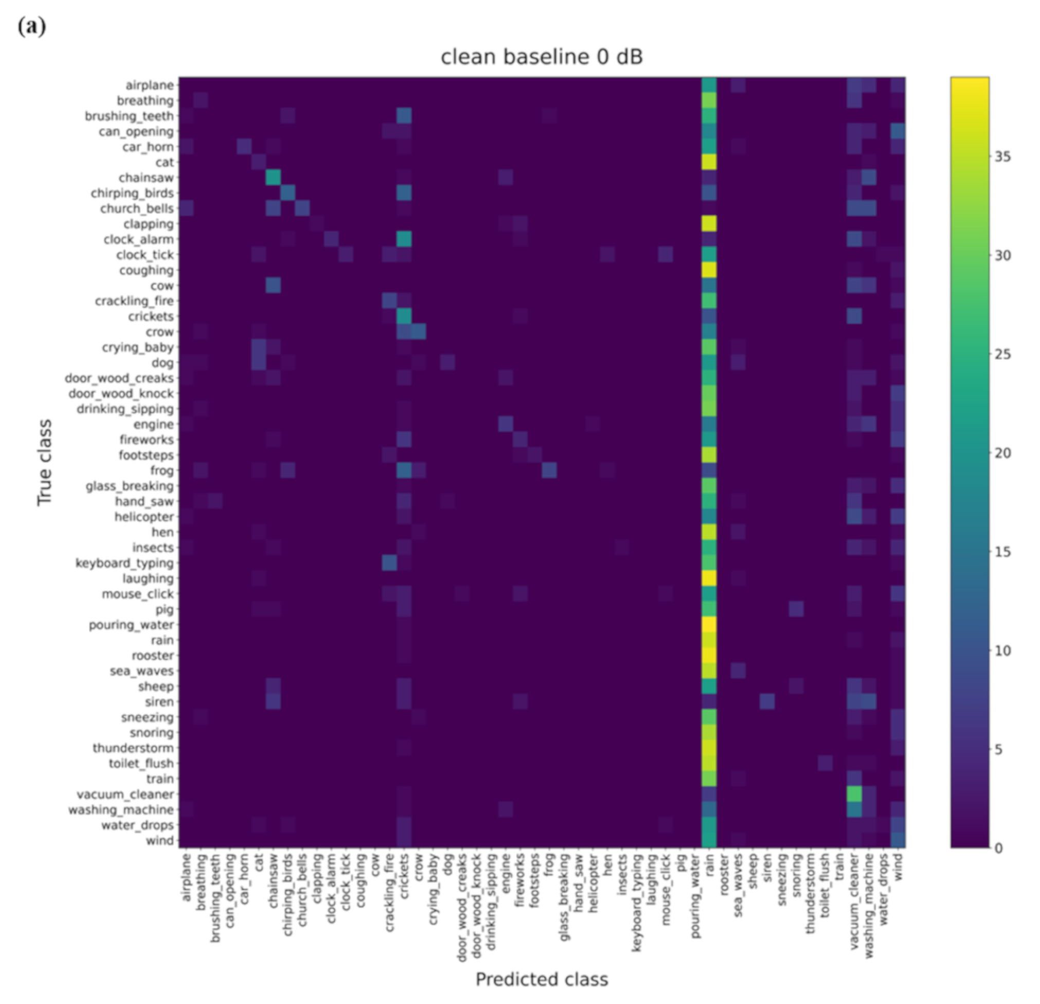
As shown in Figure 5, the aggregate confusion matrices indicated that the additive Gaussian-noise-augmented model retained a substantially stronger diagonal pattern than the clean baseline at 0 dB SNR, reflecting more correct classifications across the 50 sound classes under severe Gaussian-noise conditions. However, class-level differences were not subjected to separate statistical testing in this study. Therefore, the confusion matrices are used primarily to illustrate overall error patterns rather than to support claims about specific sound categories.

Time-shift augmentation produced results that were similar to the clean baseline across the noisy evaluation grid. Under clean evaluation, the time-shift-augmented model achieved 72.40 ± 2.50% accuracy compared with 72.05 ± 1.16% for the clean baseline, and this difference was not statistically significant (unadjusted p = 0.722165). Its mean accuracy was 62.25 ± 1.80% at 20 dB, 51.85 ± 2.02% at 15 dB, 39.25 ± 1.27% at 10 dB, 23.15 ± 1.24% at 5 dB, and 11.55 ± 1.29% at 0 dB. None of these differences relative to the clean baseline were statistically significant; the corresponding unadjusted p-values were 0.098592 at 20 dB, 0.373901 at 15 dB, 0.675049 at 10 dB, 0.963136 at 5 dB, and 0.420649 at 0 dB, and all remained nonsignificant after Holm correction. Mixup achieved the highest clean-condition accuracy, increasing mean accuracy from 72.05 ± 1.16% for the clean baseline to 75.50 ± 1.77% (unadjusted p = 0.030603); however, this difference was not statistically significant after Holm correction (adjusted p = 0.367236). Mixup  did not significantly improve performance under any noisy evaluation condition; the corresponding unadjusted p-values were 0.450999 at 20 dB, 0.507876 at 15 dB, 0.456784 at 10 dB, 0.263882 at 5 dB, and 0.395845 at 0 dB, and all remained nonsignificant after Holm correction. These findings indicate that time shifting and mixup provided limited robustness to Gaussian noise compared with direct additive-noise training.

Model	Clean	20 dB	15 dB	10 dB	5 dB	0 dB
Clean baseline	72.05 ± 1.16	63.20 ± 2.06	52.65 ± 1.01	39.05 ± 1.27	23.10 ± 1.14	10.75 ± 1.68
Noise augmented	63.75 ± 2.96	79.60 ± 2.43	78.85 ± 2.89	75.75 ± 2.39	69.65 ± 3.46	57.70 ± 4.16
Time-shift augmented	72.40 ± 2.50	62.25 ± 1.80	51.85 ± 2.02	39.25 ± 1.27	23.15 ± 1.24	11.55 ± 1.29
Mixup augmented	75.50 ± 1.77	64.50 ± 2.42	53.70 ± 2.99	40.40 ± 2.52	24.90 ± 3.18	11.80 ± 2.12

Values are reported as mean accuracy (%) ± sample standard deviation across five repeated stratified splits (random seeds 11, 22, 33, 44, and 55).

Model	Seed	Clean	20 dB	15 dB	10 dB	5 dB	0 dB
Clean Baseline	11	72.00	62.50	53.00	39.00	23.25	11.50
	22	73.75	62.75	53.25	38.75	25.00	11.00
	33	70.75	60.50	51.25	39.50	22.75	13.00
	44	72.50	66.00	53.75	40.75	22.25	8.75
	55	71.25	64.25	52.00	37.25	22.25	9.50
Noise Augmented	11	61.75	79.25	77.50	77.00	72.00	58.25
	22	59.75	76.75	75.25	72.00	66.25	51.25
	33	64.50	79.25	81.00	77.25	74.50	62.75
	44	65.75	79.25	78.00	74.75	67.75	57.25
	55	67.00	83.50	82.50	77.75	67.75	59.00
Time-Shift Augmented	11	68.75	61.50	51.75	38.50	23.50	10.00
	22	75.50	60.50	49.75	39.00	21.50	10.75
	33	71.50	61.00	50.50	38.50	22.25	13.00
	44	73.50	64.75	55.00	41.50	24.00	11.25
	55	72.75	63.50	52.25	38.75	24.50	12.75
Mixup Augmented	11	74.25	62.25	51.00	38.25	22.50	10.25
	22	76.25	65.00	52.75	41.75	27.00	11.50
	33	76.00	67.25	57.00	40.00	25.25	13.00
	44	73.25	66.25	56.75	38.00	21.00	9.50
	55	77.75	61.75	51.00	44.00	28.75	14.75

These per-seed accuracies were used to calculate the mean accuracies and sample standard deviations reported in Table 2 and the paired t-tests reported in the Results section.

Discussion

One plausible explanation for the observed robustness improvement is improved distribution matching between training and evaluation conditions. In this study, distribution matching refers to increasing the similarity between the acoustic conditions represented during training and those encountered during testing. Exposure to noisy waveforms produced YAMNet embeddings that reflected the tested corruption conditions, allowing the trainable classification head to learn a decision boundary that remained more robust as noise severity increased. This may have reduced the classifier’s dependence on clean-condition features that were less stable under Gaussian corruption and improved performance under low-SNR conditions. Prior research has shown that sound-event classification performance can degrade under mismatched acoustic conditions and that robustness-focused methods can improve classification under noise^12,13. More broadly, Salamon and Bello demonstrated that data augmentation can improve environmental sound classification and that augmentation effects may differ across sound classes³. However, the findings of the present study apply specifically to controlled Gaussian-noise conditions and do not demonstrate equivalent robustness to all forms of real-world environmental noise.

These results suggest a possible regularization and distribution-specific performance tradeoff. Gaussian-noise augmentation discouraged the classifier from relying exclusively on fine details present in clean recordings and improved generalization under matched noisy evaluation conditions. From a bias–variance perspective, this type of augmentation can be viewed as a form of regularization that may increase bias with respect to the clean-data distribution while reducing the model’s sensitivity to perturbations and training-set variation under noisy conditions. However, the present experiment did not directly decompose prediction error into formal bias and variance components. Although mean clean-condition accuracy decreased from 72.05 ± 1.16% to 63.75 ± 2.96%, this difference was not statistically significant after Holm correction. The larger standard deviation observed for the noise-augmented model at 0 dB represents greater empirical variability across the five repeated splits rather than a direct estimate of the formal variance term. Overall, noise augmentation improved average robustness under severe matched Gaussian noise while showing lower mean accuracy on uncorrupted audio, although the clean-condition difference was not statistically significant after Holm correction.

The present findings are consistent with earlier augmentation research in environmental sound classification. Salamon and Bello showed that data augmentation can improve environmental sound classification by increasing the variability of the training data and encouraging models to learn features that generalize beyond the original recordings³. In speech recognition, Ko et al. similarly demonstrated that noise-aware audio augmentation can improve performance under distorted acoustic conditions¹⁴. Although speech and environmental sounds differ in their signal structure, both studies support the broader principle that exposing a model to relevant acoustic variation during training can improve its ability to operate under related test conditions. The substantially higher low-SNR accuracy observed in the present study extends this principle to a controlled YAMNet-based ESR pipeline using synthetic Gaussian noise.

In contrast, time shifting and mixup produced much smaller improvements under Gaussian-noise evaluation. Time shifting changes the temporal position of an event without directly modeling spectral corruption, so it is more likely to improve temporal invariance than resistance to additive noise. Salamon and Bello included time shifting among the audio augmentations evaluated for environmental sound classification and showed that the effect of individual augmentation methods can vary across sound classes³. Mixup is a regularization method that trains a model on convex combinations of pairs of examples and their corresponding labels, encouraging smoother behavior between training samples⁴. In the present study, mixup produced higher mean clean-condition accuracy than the clean baseline, but this difference was not statistically significant after Holm correction, and mixup did not improve accuracy at any noisy SNR level. These findings suggest that neither temporal displacement nor embedding interpolation directly prepared the classifier for the Gaussian acoustic corruption used during evaluation.

Limitations and Future Work

One limitation of this study is that the noisy training and evaluation conditions were generated using synthetic zero-mean Gaussian noise. This approach enabled controlled and reproducible comparisons across SNR levels, but Gaussian noise does not capture the full complexity of real-world acoustic interference. Environmental noise may be non-stationary and may include competing sound sources, reverberation, microphone characteristics, and changes in source distance. Therefore, the absolute performance values obtained under the controlled Gaussian-noise conditions should not be interpreted as direct estimates of performance in all real-world environments.

Another limitation of this research is related to the size and diversity of the dataset used. The dataset used in this research has a small number of samples per class and is dominated by short, curated audio examples. Although this enables a controlled benchmarking process, it does not fully capture the diversity of environmental sounds as they are encountered in real-world recordings, where environmental sounds can be overlapping and presented in more complex acoustic scenarios. Furthermore, the experiments were carried out using a single dataset, which could affect the generalizability of the results to other environmental sound classification datasets with different characteristics. Future work could evaluate these augmentation strategies on larger and more diverse datasets such as FSD50K, which contain substantially greater acoustic variability than ESC-50²⁶.

Lastly, the models used in this research utilized embeddings derived from a pre-trained audio representation model as opposed to training the model end-to-end on raw audio. Although transfer learning facilitates high-performance results using a small amount of data, it may limit the ability of the classifier to fully capture the dataset used in this research. Future research could investigate these approaches using larger and more diverse datasets and explore other augmentation techniques to further enhance the robustness of the models.

Another limitation is that the augmentation strategies were not all applied at the same stage of the processing pipeline. Additive Gaussian noise and time shifting were applied to waveforms before YAMNet embedding extraction, whereas mixup was applied to the extracted embeddings. Therefore, differences involving mixup may reflect both the augmentation strategy itself and the stage at which the augmentation was applied. Future work could compare waveform-level and embedding-level implementations under otherwise identical conditions.

Because the five repeated stratified train-validation-test splits may contain overlapping samples, the resulting split-level accuracy estimates are not guaranteed to be fully independent. The paired t-tests therefore provide an approximate comparison across repeated splits rather than a formal independent-sample inference. To address multiplicity across the 18 model-by-condition comparisons, the Holm procedure was applied to the paired-test p-values. The main noise-augmentation result remained significant at all five noisy SNR levels after correction, while the clean-condition noise comparison and the clean-condition mixup comparison were no longer statistically significant.

Although all models used the same maximum epoch limit, batch size, early-stopping criterion, and validation-based stopping procedure, the actual training duration differed across conditions. In particular, the noise-augmented models generally trained for more epochs before early stopping than the clean and time-shift models. This difference in optimization exposure is a potential confounding factor and was not independently controlled in the present study. However, the noise-augmented model showed lower clean-condition accuracy despite the additional training while producing large improvements specifically under matched Gaussian-noise evaluation conditions, which is consistent with the augmentation strategy contributing to the observed robustness gains rather than the gains being attributable solely to longer training. Future work could control the number of optimization updates directly across augmentation conditions.

Conclusion

This study examined the effects of additive Gaussian noise, time shifting, and mixup on the robustness of an environmental sound recognition system based on pretrained YAMNet embeddings. Across five repeated stratified train-validation-test splits, additive noise augmentation produced the strongest performance under every noisy evaluation condition. After Holm correction across the 18 model-by-condition comparisons, additive Gaussian-noise augmentation remained significantly better than the clean baseline at all five noisy SNR levels. Under clean evaluation, the noise-augmented model had lower mean accuracy than the clean baseline, but this difference was not statistically significant after Holm correction. Time shifting did not significantly improve noisy-condition accuracy. Mixup showed higher mean clean-condition accuracy than the clean baseline, but this difference was not statistically significant after Holm correction, and mixup did not improve robustness under the noisy evaluation conditions.

The results of this study emphasize the need to develop robust training strategies for environmental sound recognition systems. In uncontrolled environments, acoustic signals may contain overlapping sound classes and background noise that can affect the classification process. Therefore, incorporating additive Gaussian-noise augmentation during training can improve robustness when environmental sound recognition systems are evaluated under similar noisy conditions. These findings suggest that augmentation strategies can play an important role in improving robustness under controlled Gaussian-noise conditions.

In future work, this study can be extended by evaluating the effectiveness of the augmentation strategies using larger datasets. In particular, the dataset can include recordings containing naturally occurring environmental interference, overlapping sources, reverberation, and device variation. Moreover, future research can also introduce new strategies to improve the robustness of ESR systems.

References

1. K. J. Piczak, “ESC-50: Dataset for environmental sound classification,” in Proc. ACM Int. Conf. Multimedia (ACM MM), 2015, pp. 1015–1018 [↩] [↩] [↩]
2. J. Salamon, C. Jacoby, and J. P. Bello, “UrbanSound8K: A dataset of urban sound clips,” in Proc. ACM Int. Conf. Multimedia (ACM MM), 2014, pp. 1041–1044 [↩] [↩] [↩]
3. J. Salamon and J. P. Bello, “Deep convolutional neural networks and data augmentation for environmental sound classification,” IEEE Signal Processing Letters, vol. 24, no. 3, pp. 279–283, 2017 [↩] [↩] [↩] [↩] [↩] [↩]
4. H. Zhang, M. Cissé, Y. N. Dauphin, and D. Lopez-Paz, “mixup: Beyond empirical risk minimization,” in Proc. Int. Conf. Learning Representations (ICLR), 2018 [↩] [↩] [↩] [↩]
5. D. S. Park et al., “SpecAugment: A simple data augmentation method for automatic speech recognition,” in Proc. Interspeech, 2019, pp. 2613–2617 [↩] [↩]
6. A. Guzhov, F. Raue, J. Hees, and A. Dengel, “ESResNet: Environmental Sound Classification Based on Visual Domain Models,” Pattern Recognition Letters, vol. 144, pp. 50–57, 2021 [↩] [↩]
7. Q. Kong, Y. Cao, T. Iqbal, Y. Wang, W. Wang, and M. D. Plumbley, “PANNs: Large-Scale Pretrained Audio Neural Networks for Audio Pattern Recognition,” IEEE/ACM TASLP, vol. 28, pp. 2880–2894, 2020 [↩] [↩]
8. S. Hershey et al., “CNN architectures for large-scale audio classification,” in Proc. IEEE Int. Conf. Acoustics, Speech and Signal Processing (ICASSP), 2017, pp. 131–135 [↩] [↩] [↩]
9. J. F. Gemmeke et al., “AudioSet: An ontology and human-labeled dataset for audio events,” in Proc. IEEE Int. Conf. Acoustics, Speech and Signal Processing (ICASSP), 2017, pp. 776–780 [↩]
10. Google Research, “YAMNet: Pretrained audio event classifier,” 2020. [Online]. Available: https://github.com/tensorflow/models/tree/master/research/audioset/yamnet [↩]
11. A. van den Oord, Y. Li, and O. Vinyals, “Representation learning with contrastive predictive coding,” arXiv preprint arXiv:1807.03748, 2018 [↩]
12. J. Dennis, H. D. Tran, and H. Li, “Spectrogram image feature for sound event classification in mismatched conditions,” IEEE Signal Processing Letters, vol. 18, no. 2, pp. 130–133, 2011 [↩] [↩] [↩]
13. S. McLoughlin, H. Zhang, Z. Xie, Y. Song, and W. Xiao, “Robust sound event classification using deep neural networks,” IEEE/ACM Transactions on Audio, Speech, and Language Processing, vol. 23, no. 3, pp. 540–552, 2015 [↩] [↩] [↩]
14. T. Ko, V. Peddinti, D. Povey, and S. Khudanpur, “Audio augmentation for speech recognition,” in Proc. Interspeech, 2015, pp. 3586–3589 [↩] [↩] [↩]
15. I. Goodfellow, Y. Bengio, and A. Courville, Deep Learning, MIT Press, 2016 [↩]
16. Y. Ganin et al., “Domain-Adversarial Training of Neural Networks,” Journal of Machine Learning Research, vol. 17, no. 59, pp. 1–35, 2016 [↩]
17. I. J. Goodfellow, J. Shlens, and C. Szegedy, “Explaining and Harnessing Adversarial Examples,” in Proc. International Conference on Learning Representations (ICLR), 2015 [↩]
18. Y. Gal and Z. Ghahramani, “Dropout as a Bayesian Approximation: Representing Model Uncertainty in Deep Learning,” in Proc. International Conference on Machine Learning (ICML), 2016, pp. 1050–1059 [↩]
19. T. Heittola, A. Mesaros, A. Eronen, and T. Virtanen, “Context-dependent sound event detection,” in Proc. Detection and Classification of Acoustic Scenes and Events (DCASE) Workshop, 2013 [↩]
20. K. J. Piczak, “Environmental sound classification with convolutional neural networks,” in Proc. IEEE International Workshop on Machine Learning for Signal Processing (MLSP), 2015, pp. 1–6 [↩]
21. Y. Tokozume and T. Harada, “Learning environmental sounds with end-to-end convolutional neural network,” in Proc. IEEE International Conference on Acoustics, Speech and Signal Processing (ICASSP), 2017, pp. 2721–2725 [↩]
22. K. Koutini et al., “Receptive-Field-Regularized CNN Variants for Acoustic Scene Classification,” DCASE Workshop, 2021 [↩]
23. J. Shorten and T. M. Khoshgoftaar, “A Survey on Image Data Augmentation for Deep Learning,” Journal of Big Data, vol. 6, no. 60, 2019 [↩]
24. J. Wei and K. Zou, “EDA: Easy Data Augmentation Techniques for Boosting Performance on Text Classification Tasks,” in Proc. Conference on Empirical Methods in Natural Language Processing (EMNLP), 2019 [↩]
25. B. McFee et al., “librosa: Audio and music signal analysis in Python,” in Proc. Python in Science Conf. (SciPy), 2015, pp. 18–24 [↩]
26. E. Fonseca et al., “FSD50K: An Open Dataset of Human-Labeled Sound Events,” IEEE/ACM TASLP, vol. 30, pp. 829–852, 2022 [↩]