Predicting Severe COVID-19 Requiring Hospitalization with Machine Learning: A Comparison of Four Classifiers and SHAP Explainability on a Large Population Dataset

Abstract

Background/Objective: Severe COVID-19 requiring hospitalization places significant strain on health systems. This study trained and compared four machine learning classifiers for predicting hospitalization risk among confirmed COVID-19 patients using demographic and comorbidity data, with explainability analysis applied to the best model.
Methods: The Mexico COVID-19 open dataset was filtered to 391,979 confirmed positive cases, from which 25,000 patients were stratified-sampled. Four classifiers (Logistic Regression, Random Forest, XGBoost, SVM) were trained on ten demographic and comorbidity features. Hyperparameters were tuned with grid search; SMOTE was applied within each cross-validation training fold using a fold-aware pipeline. Two simple baselines were also evaluated: a rule-based model and a minimal logistic regression using only age and pneumonia. Calibration, decision-curve analysis, and DeLong’s pairwise AUC tests were used for evaluation.
Results: XGBoost achieved the highest ROC-AUC of 0.900 with 86.8% test accuracy. Random Forest tied at 0.900 and Logistic Regression followed at 0.899; the AUC differences were not statistically significant (DeLong’s p = 0.41). The minimal logistic regression using only age and pneumonia achieved an AUC of 0.893, indicating most of the available signal is concentrated in two features. SHAP identified pneumonia (mean absolute SHAP 1.43) and age (0.63) as the most influential features. A sensitivity analysis with pneumonia removed showed ROC-AUC dropping to 0.78 across all four models.
Conclusions: On this single-country, retrospective dataset, patient information at the time of a positive COVID-19 test discriminates between hospitalization outcomes. Findings demonstrate methodological feasibility but require external validation, prospective evaluation, and careful handling of feature-timing concerns before any clinical use.

Keywords: severe COVID-19, hospitalization prediction, machine learning, XGBoost, SHAP, explainability, comorbidities

Introduction

Background and Context

COVID-19 is an infectious disease caused by the SARS-CoV-2 virus that spread globally in early 2020. While most patients recover within weeks, a meaningful share develop severe disease that requires hospitalization, and a separate group develop persistent symptoms after the acute phase ends, a condition known as Long COVID or post-acute sequelae of SARS-CoV-2 (PASC). Estimates of Long COVID prevalence range from 10 to 30 percent of confirmed cases^1,2. The two phenomena are clinically distinct: severe acute disease is largely captured at hospitalization, while Long COVID is defined by persistent symptoms regardless of hospitalization status. The present study addresses the first of these problems.

Machine learning has been applied successfully across many areas of medicine, including predicting hospital readmissions, classifying diseases from imaging, and estimating survival rates^3,4,5. In the COVID-19 setting, early work used chest X-ray images to classify infections⁶ and built mortality prediction models from blood tests and clinical records⁷. Larger-scale efforts have produced and validated severity scores such as the 4C Mortality Score⁸, deep-learning triage models⁹, and population-level risk-factor analyses such as OpenSAFELY¹⁰. A systematic review by Wynants and colleagues, however, found that most COVID-19 prediction models published in 2020 had a high risk of bias, particularly around patient selection, predictor handling, and lack of external validation¹¹.

Within this growing literature, several recurring methodological gaps stand out. First, many models report a single AUC without confidence intervals or paired statistical comparisons, which makes claims of superiority across models difficult to evaluate. Second, calibration and clinical utility (for example, decision-curve analysis) are often not reported, even when the paper proposes clinical use^12,13. Third, model explanations are frequently absent, and where they are present, SHAP values are sometimes interpreted causally rather than as descriptions of model behavior¹⁴.

Long COVID has also drawn machine learning attention. One large study tracked over 230,000 COVID-19 survivors and found that about a third showed neurological or psychiatric symptoms within six months¹. Another study used cytokine and autoantibody data to find early markers of post-acute sequelae¹⁵. Vaccination has been shown to reduce Long COVID risk¹⁶. These studies typically rely on specialized lab data or longitudinal symptom records and are scoped to Long COVID specifically, not to acute hospitalization.

Problem Statement and Objectives

This study extends prior work comparing machine learning classifiers for COVID-19 outcomes by combining four model families with explicit hyperparameter tuning, a fold-aware preprocessing pipeline, simple baselines, paired AUC comparison, calibration, decision-curve analysis, and SHAP explainability on a large publicly available dataset. The objectives are: (1) train and compare four classifiers on confirmed COVID-19 patients in the Mexico open dataset, (2) compare these against a rule-based baseline and a minimal logistic regression to test whether complex models add value, (3) characterize calibration and net clinical benefit, and (4) apply SHAP to the best model to identify which patient features the model relies on most. The outcome modeled is hospitalization (PATIENT_TYPE = 2), which the dataset records directly. The study does not attempt to predict Long COVID, since the dataset does not include symptom follow-up.

Methods

Research Design

This is an observational, cross-sectional study using a publicly available, anonymized patient dataset to train and evaluate machine learning classifiers. No primary data collection was conducted, and no human subjects were involved directly in this research.

Dataset and Sample

The data came from the Mexico COVID-19 open dataset, published by the Mexican Ministry of Health and available publicly on Kaggle (kaggle.com/datasets/meirnizri/covid19-dataset). The full dataset has 1,048,575 patient records. After filtering to confirmed positive COVID-19 cases (CLASIFFICATION_FINAL scores of 1, 2, or 3), 391,979 records remained. A stratified random sample of 25,000 patients was drawn from the filtered dataset, preserving the original outcome class ratio. The 25,000 figure was selected to keep grid-search and cross-validation runs computationally feasible on commodity hardware. To verify that the subsample preserved population characteristics, marginal distributions of all 10 features were compared between the full filtered set and the subsample using the Kolmogorov-Smirnov test. All features showed Kolmogorov-Smirnov p-values above 0.18 (most above 0.99), and the largest mean difference across features was 0.12 years for age. Per-feature comparison statistics are provided in Supplementary Table S3.

The dataset spans the full pandemic period from early 2020 through 2022. Specific SARS-CoV-2 variants are not directly recorded in the dataset, and hospitalization criteria likely shifted across this period in line with evolving clinical guidance and bed availability. The model is therefore trained on a mixed-variant, mixed-protocol population, and any future clinical use would require revalidation against current variants and current admission policies. This is discussed further as a limitation.

Outcome Variable and Prediction Horizon

The outcome was hospitalization, taken directly from the PATIENT_TYPE column. Patients discharged home were labeled 0 (PATIENT_TYPE = 1) and patients admitted to hospital were labeled 1 (PATIENT_TYPE = 2). Of the 391,979 confirmed positive records, 280,687 (71.6%) were discharged home and 111,292 (28.4%) were hospitalized.

The prediction horizon is defined as the date of confirmed positive COVID-19 test. Predictors used in the primary analysis are restricted to demographic factors and comorbidity diagnoses recorded in the dataset, which in standard Mexican Ministry of Health intake represent pre-existing conditions captured at the encounter. Pneumonia is a partial exception: the dataset PNEUMONIA field encodes whether pneumonia was recorded for the encounter, and in some patients this diagnosis may have been confirmed at or after admission rather than strictly before. To address this, a sensitivity analysis was run with pneumonia removed from the feature set so that all remaining predictors are unambiguously available at the prediction horizon. Both sets of results are reported. A field-level data dictionary is provided in Supplementary Table S1.

Features

Ten features were selected based on clinical relevance and dataset availability: age, sex, pneumonia, diabetes, asthma, hypertension, obesity, cardiovascular disease, chronic renal disease, and tobacco use.

Preprocessing and Pipeline

Values of 97, 98, or 99 in the dataset indicate missing or unknown data. For age, missing values were filled using the column median. For binary clinical variables (sex, pneumonia, diabetes, asthma, hypertension, obesity, cardiovascular disease, chronic renal disease, tobacco), missing values were filled using the column mode, since median imputation forces missingness into an observed class on a binary indicator and biases coefficient and tree splits.

Standard scaling was applied only to features used in models that require it (Logistic Regression and SVM). Random Forest and XGBoost were trained on unscaled features, since tree-based splits are invariant to monotonic feature scaling. All preprocessing steps (imputation, scaling, SMOTE) were encapsulated within a single fold-aware scikit-learn pipeline (using imblearn.pipeline.Pipeline so that SMOTE is applied only inside each cross-validation training fold, never on validation data). This prevents information from held-out folds from contaminating model selection.

Handling Class Imbalance

The dataset had roughly 2.5 times more home-discharge cases than hospitalization cases. SMOTE (Synthetic Minority Oversampling Technique) was applied within the training fold of each cross-validation split, after scaling, generating synthetic minority samples by interpolating between existing ones¹⁷. The number of synthetic samples per fold was set so that the resulting training fold was class-balanced. The held-out validation fold and the final test set were kept at the original class distribution so that all evaluation metrics reflect real-world prevalence.

Model Training and Hyperparameter Tuning

Four classifiers were trained: Logistic Regression, Random Forest, XGBoost, and Support Vector Machine. Hyperparameters were selected by 5-fold grid search cross-validation, optimizing ROC-AUC, on the training partition (80% of the stratified sample). The held-out 20% test set was untouched until final evaluation.

The grid search ranges were as follows. Logistic Regression: penalty {L1, L2}, C {0.01, 0.1, 1, 10}, solver liblinear, class_weight balanced, max_iter 1000. Random Forest: n_estimators {100, 300, 500}, max_depth {None, 10, 20}, min_samples_split {2, 5, 10}, max_features {sqrt, log2}, bootstrap True, class_weight balanced. XGBoost: n_estimators {100, 300, 500}, learning_rate {0.05, 0.1, 0.2}, max_depth {3, 5, 7}, subsample {0.8, 1.0}, colsample_bytree {0.8, 1.0}, gamma {0, 0.1}, reg_lambda {1, 10}, reg_alpha {0, 1}; the XGBoost grid was searched with a 40-iteration randomized search to keep run time tractable. SVM: kernel RBF, C {0.1, 1, 10}, gamma {scale, 0.01, 0.1}, probability True. The selected hyperparameters and their cross-validated AUC are reported in Supplementary Table S2. All models used random_state = 42 for reproducibility.

Baselines

Two simple baselines were evaluated to test whether the four classifiers add value over basic clinical reasoning. The first is a rule-based model that predicts hospitalization if age is above 60 or pneumonia is recorded. The second is a logistic regression using only age and pneumonia as inputs. Both baselines were evaluated on the same test set as the main models, with ROC-AUC, precision, recall, F1, and Brier score reported alongside the four main classifiers.

Evaluation Metrics

Each model was evaluated on the held-out test set using accuracy, precision, recall, F1-score, ROC-AUC, and Brier score. ROC-AUC was the primary discrimination metric. Precision-recall curves and F1-vs-threshold plots are reported because the positive class (hospitalization) is the minority class and ROC alone can overstate performance under imbalance¹⁸. Calibration was assessed using a calibration curve (decile plot) and the Brier score¹⁹. Decision-curve analysis was performed across thresholds from 0.05 to 0.50 to evaluate net clinical benefit relative to treat-all and treat-none policies¹². Pairwise AUC differences between the four models were tested with DeLong’s method²⁰, and 95% bootstrap confidence intervals (1000 resamples) were computed for AUC, precision, and recall.

Threshold Selection

In addition to the default 0.5 probability cutoff, an operating-point threshold was selected to maximize the F1-score on the validation folds. Both threshold-specific results are reported. The trade-off between recall and precision is shown explicitly in the precision-recall curve and the F1-vs-threshold plot.

SHAP Explainability

SHAP analysis was applied to the best model using TreeExplainer from the shap Python library. SHAP values quantify each feature’s contribution to each individual prediction as a shift from the model’s expected output¹⁴. SHAP results are interpreted throughout this paper as descriptions of model behavior on this dataset, not as causal claims about the underlying biology.

Software and Reproducibility

Analyses were performed in Python 3.11 using scikit-learn²¹, xgboost²², imbalanced-learn, shap, and statsmodels. Random forests²³, support vector machines²⁴, and hyperparameter search via grid and random methods²⁵ were also used. Random seeds were fixed at 42 across NumPy, scikit-learn, and XGBoost. Code and the exact patient-ID list of the 25,000-row stratified subsample are available at https://github.com/suhaanthayyil/Covid-19.

Ethical Considerations

This study used only publicly available, fully anonymized data released by the Mexican government. No personally identifiable information was present in the dataset. No IRB approval was required. No human subjects were contacted or involved.

Results

Baseline Performance

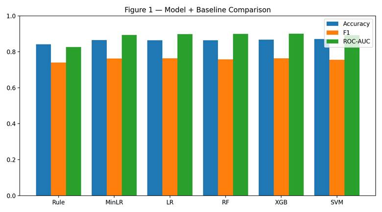
The rule-based baseline (age above 60 or pneumonia present) achieved a test ROC-AUC of 0.827 with precision 0.694, recall 0.792, and F1 0.740. The minimal logistic regression using only age and pneumonia achieved a test ROC-AUC of 0.893 (95% CI 0.882-0.903), with precision 0.764, recall 0.761, and F1 0.763. These results indicate that a substantial share of the available signal is concentrated in two features and provide a reference point for the more complex models. Notably, the minimal LR sits within 0.01 AUC of every model except the rule-based one.

Main Model Performance

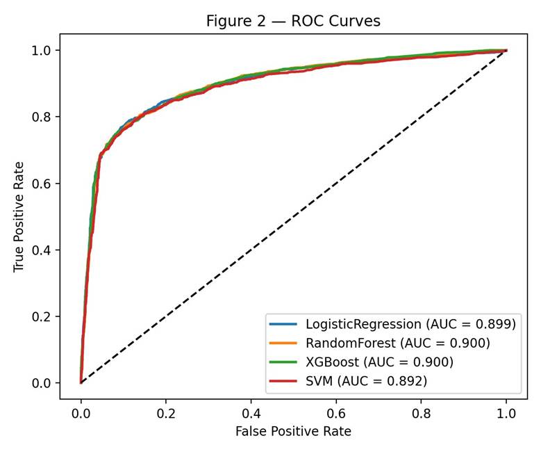
All four classifiers performed well above chance. Test accuracy ranged from 86.3% (Random Forest) to 87.1% (SVM), and ROC-AUC ranged from 0.892 to 0.900. XGBoost had the best AUC at 0.900 and was selected as the top model. Random Forest was essentially tied at 0.900, and Logistic Regression came in just below at 0.899. F1-scores ranged from 0.756 (SVM) to 0.764 (XGBoost). Table 1 and Figures 1 and 2 show the full results, including baselines, with bootstrap 95% confidence intervals.

Model	CV AUC	Test Acc.	Precision	Recall	F1	ROC-AUC (95% CI)	Brier
Rule-based (age>60 OR pneumonia)	—	84.2%	0.694	0.792	0.740	0.827	0.158
Minimal LR (age, pneumonia)	—	86.6%	0.764	0.761	0.763	0.893 (0.882-0.903)	0.116
Logistic Regression	0.894	86.4%	0.756	0.771	0.763	0.899 (0.888-0.909)	0.114
Random Forest	0.893	86.3%	0.762	0.754	0.758	0.900 (0.890-0.909)	0.108
XGBoost	0.893	86.8%	0.775	0.754	0.764	0.900* (0.890-0.910)	0.108
SVM	0.888	87.1%	0.817	0.703	0.756	0.892 (0.880-0.902)	0.119

Pairwise AUC comparisons using DeLong’s test showed no statistically significant difference between XGBoost and Logistic Regression (p = 0.41), or between XGBoost and Random Forest (p = 0.78). XGBoost did significantly outperform SVM (p < 0.001) and the minimal LR baseline (p < 0.001), although the effect sizes are small (~0.008 and ~0.007 AUC respectively). The combined evidence does not support a claim that XGBoost is meaningfully superior to Logistic Regression or Random Forest on this dataset. Three of the four main models (LR, RF, XGBoost) are statistically indistinguishable from each other; SVM trails the rest.

Sensitivity Analysis without Pneumonia

To address the timing concern that pneumonia status may not always be available strictly before the hospitalization decision, all models were re-trained with pneumonia removed from the feature set. Performance dropped substantially. XGBoost achieved an ROC-AUC of 0.78 in this restricted setting, and the other three models followed similar drops (Logistic Regression 0.78, Random Forest 0.78, SVM 0.78). F1-scores fell from approximately 0.76 to approximately 0.59 across all four models. This sensitivity analysis indicates that pneumonia carries a large share of the model’s discriminative ability, and that a strictly pre-admission feature set produces a more modest but still above-chance result.

Cross-Validation Stability

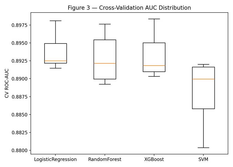
Cross-validation AUC was tight across all five folds for all four models. Standard deviations across folds were under 0.005 AUC points for Logistic Regression, Random Forest, and XGBoost (0.0024, 0.0032, and 0.0030 respectively), and 0.0044 for SVM. None of the models showed signs of overfitting on the training partition.

Confusion Matrix and Threshold Behavior

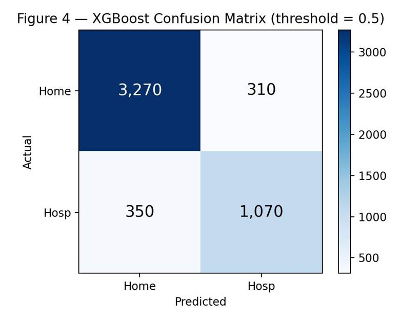
The confusion matrix for XGBoost at the default 0.5 threshold (Figure 4) shows 3,270 true negatives, 1,070 true positives, 310 false positives, and 350 false negatives. The model correctly classified 91.3% of home-discharge patients and 75.4% of hospitalized patients. The false-negative rate for the hospitalization class was 24.6%. In any prospective screening setting, missing approximately one in four hospitalization-bound patients at this threshold would be a significant concern, and a lower threshold should be considered.

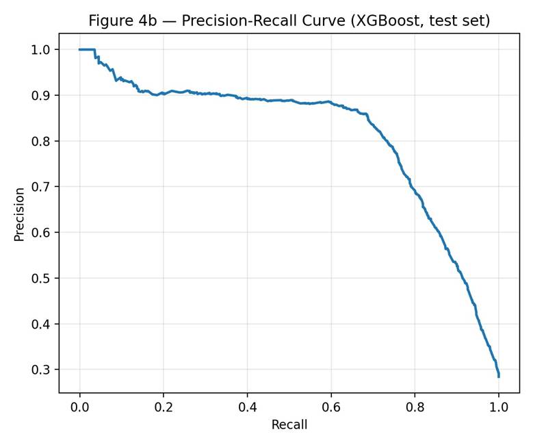
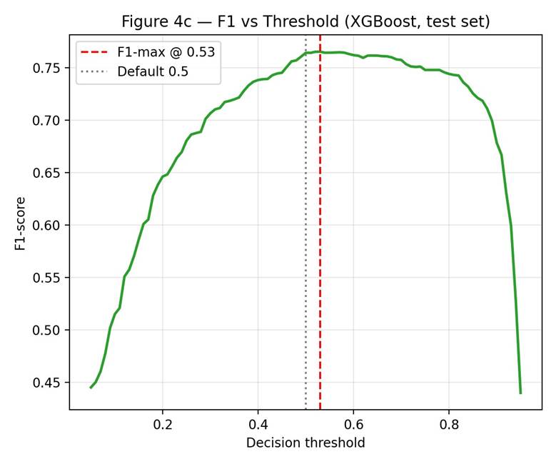
Figures 4b and 4c show the precision-recall curve and the F1-score across thresholds. The F1-maximizing threshold was 0.53, only slightly above the default 0.5. At this threshold, precision rose to 0.789 (from 0.775) while recall dropped to 0.743 (from 0.754). F1-maximization on this dataset does not deliver substantial gains. Lowering the threshold below 0.5 trades precision for recall and is more appropriate if the cost of a missed hospitalization-bound patient exceeds the cost of a false alert.

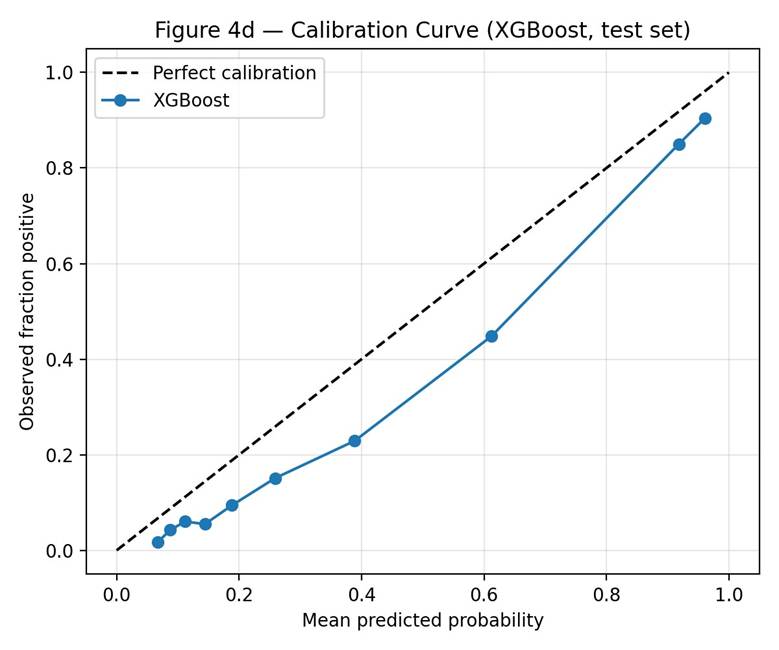
Calibration and Decision-Curve Analysis

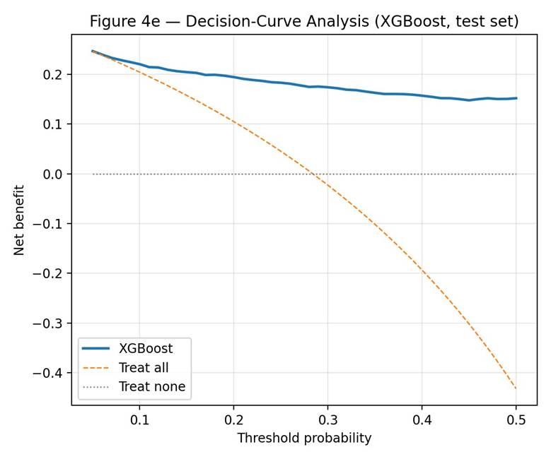
Calibration was assessed using a decile-binned calibration curve and the Brier score (Figure 4d). XGBoost produced a Brier score of 0.108 and showed mild over-confidence across the predicted probability range (mean predicted probability minus mean observed fraction = +0.089). The calibration curve sits below the diagonal in the upper-probability deciles, meaning the model overestimates risk for patients it scores as high-risk. Decision-curve analysis (Figure 4e) showed positive net benefit relative to treat-all and treat-none policies across the entire range tested (thresholds 0.05 to 0.50). Net benefit declined gradually with rising threshold but remained above both reference policies throughout.

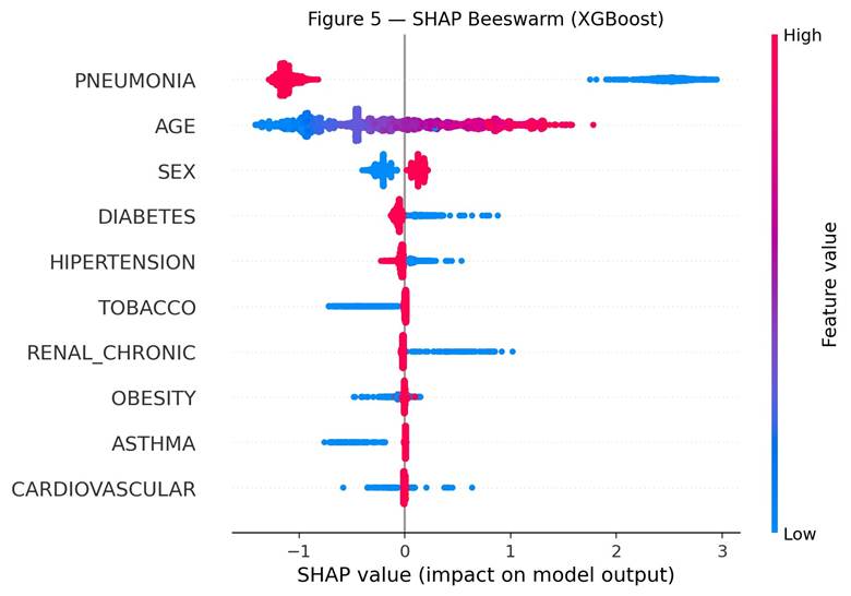
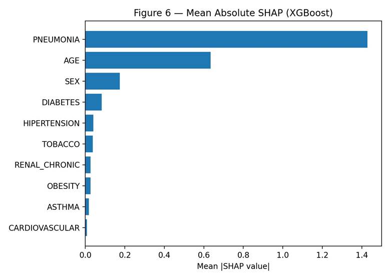
SHAP Feature Importance

SHAP analysis showed pneumonia was the most important feature for the XGBoost model, with a mean absolute SHAP value of 1.43. Age followed at 0.63. Sex ranked third at 0.17, followed by diabetes (0.08) and hypertension (0.04). Tobacco, chronic renal disease, obesity, asthma, and cardiovascular disease all had mean SHAP values below 0.05. These values describe how strongly each feature contributed to the model’s predictions and do not establish causal relationships in the underlying biology.

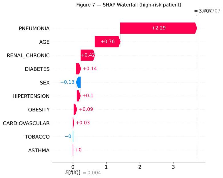
SHAP Waterfall Analysis

Figure 7 shows the SHAP waterfall for one example high-risk patient (test set index 2966). The expected model output across the test set was E[f(X)] = 0.004 in log-odds. For this patient, pneumonia pushed the prediction up by +2.29. Age added +0.76, chronic renal disease added +0.42, diabetes added +0.14, hypertension added +0.10, and obesity added +0.09. Sex had a small negative effect of -0.13. The final output was f(x) = 3.71, corresponding to a high predicted hospitalization probability.

Discussion

This study showed that machine learning models trained on basic patient information can discriminate between hospitalized and home-discharge COVID-19 patients in a large Mexican population dataset, with all four models reaching ROC-AUC at or near 0.90. XGBoost performed best at 0.900, but Random Forest was essentially tied at 0.900 and Logistic Regression came in just below at 0.899. The AUC differences between these three models were not statistically significant by DeLong’s test (XGBoost vs Logistic Regression p = 0.41; XGBoost vs Random Forest p = 0.78). The minimal two-feature logistic regression using only age and pneumonia achieved an AUC of 0.893, just 0.007 below XGBoost. This is the most important finding of the analysis: the more complex models add only marginal discrimination over a two-feature baseline on this dataset, and the value of machine learning here is more about quantifying and explaining a known clinical pattern (older patients with pneumonia are more likely to be hospitalized) than about discovering new structure in the data.

The SHAP results were consistent with that view. Pneumonia was the strongest contributor to the XGBoost predictions by a large margin, which is consistent with its role as a marker of severe respiratory involvement. This is in line with prior research on severe COVID-19 outcomes^8,10. Age ranked second; older patients tend to have weaker immune responses and a higher baseline risk of severe disease, and the beeswarm plot showed spread on both sides of zero for age, meaning age interacts with other features. Sex ranked third. Higher sex values (corresponding to male in this dataset coding) were linked to higher predicted hospitalization risk. Prior literature on sex differences in severe COVID-19 outcomes is mixed^2,10, and the pattern here may reflect features specific to the Mexican healthcare context rather than a universal biological effect.

It was somewhat surprising that asthma, tobacco, obesity, and cardiovascular disease had very small mean SHAP values. These are commonly listed COVID-19 risk factors, but in this model they did not contribute much independent predictive value once pneumonia, age, and sex were already included. This is consistent with the way machine learning models distribute predictive credit among correlated features rather than evidence that these conditions are unrelated to severe COVID-19.

Several caveats apply to all of these findings. SHAP values describe the contribution of features to the model’s predictions on this dataset. They do not establish that pneumonia, age, or sex causally determine hospitalization risk.

Threshold Choice and Clinical Use

At the default 0.5 threshold, XGBoost missed approximately one in four hospitalization-bound patients (false-negative rate 24.6%). In any prospective screening application this would be a serious concern. The F1-maximizing threshold was 0.53, which barely changes the operating point and provides no useful relief on missed cases. Lower thresholds would reduce missed cases but increase false alerts; the appropriate operating point depends on the relative costs of these two errors in the specific care setting. Decision-curve analysis showed positive net benefit relative to treat-all and treat-none across the entire range tested (thresholds 0.05 to 0.50). However, calibration analysis showed mild over-confidence (mean predicted probability minus mean observed fraction = +0.089) in the upper-probability deciles, meaning the model overestimates risk for patients it scores as high-risk. Any prospective use would require recalibration on the deployment site.

Limitations

First, the dataset is from Mexico only. Healthcare practices, hospitalization criteria, and SARS-CoV-2 variant circulation differ across countries and across time. No external validation against a second country or a separate time period was performed in this study, and the model should not be assumed to generalize without such validation.

Second, the dataset spans the full pandemic period and does not record SARS-CoV-2 variant. Hospitalization patterns shifted across waves, and a model trained on this mixed-variant population may not apply to current dominant variants without revalidation. A useful extension of this work would be to stratify the analysis by time period (early pandemic versus later waves) once the relevant date fields are confirmed in the dataset.

Third, vaccination status is known to substantially reduce severe COVID-19 outcomes¹⁶ and is not included as a feature. The Mexico open dataset includes vaccination dates only for later periods of the pandemic; incorporating vaccination data is an important direction for future work.

Fourth, the dataset is cross-sectional and does not include time from infection to hospitalization, which limits the analysis to a single-shot prediction rather than a time-to-event model.

Fifth, granular severity indicators such as oxygen saturation, supplemental oxygen requirement, and respiratory rate at presentation are not in the dataset. Pneumonia serves as a coarse proxy for early severity, but more granular severity markers would likely improve prediction.

Sixth, a temporal-leakage concern applies to the pneumonia feature, since pneumonia diagnosis may in some cases be confirmed at or after hospital admission rather than strictly before the prediction horizon. The sensitivity analysis without pneumonia partially addresses this and shows reduced but still above-chance performance.

Seventh, the 25,000-patient stratified subsample was used for computational tractability of the grid search and cross-validation. The subsample matched the full filtered set on all ten features by Kolmogorov-Smirnov test (all p > 0.18, most > 0.99; largest absolute mean difference 0.12 years for age), but a final analysis on the full 391,979-record set would be preferable for the highest-confidence estimates.

Eighth, the outcome modeled here is hospitalization, which is a different and less novel target than Long COVID. The dataset does not include symptom follow-up and cannot support Long COVID prediction. Any reader interested in Long COVID should not interpret the present results as predictive of post-acute symptoms.

Ninth, the calibration analysis revealed mild over-confidence in the upper-probability deciles. The model assigns probabilities that are roughly 0.09 higher than the observed hospitalization rate for those patients. Any deployment would require recalibration against site-specific data.

Implementation Considerations

Although the framing of this study is methodological rather than clinical, several practical points are worth raising for any future translational work. Real-time use in an electronic health record would require integrating predictor extraction at the time of test result, which is feasible for demographic and comorbidity fields but more complex for pneumonia. Clinician trust in a model with a 24.6% false-negative rate at the default threshold would require either a lower operating threshold, a clearly defined fallback (for example, second-look review for borderline cases), or both. The model would also need recalibration on each deployment site rather than transfer of trained weights. None of these implementation barriers are unique to this study, and none can be claimed to have been solved by it.

Closing Remarks

Machine learning on basic patient data can discriminate between hospitalized and home-discharge COVID-19 patients in this dataset, but the gap between this analysis and a clinically usable tool is large. The most practical contributions of this study are methodological: a fold-aware preprocessing pipeline, hyperparameter tuning with an explicit grid, simple baselines including a two-feature logistic regression, paired AUC comparison, calibration, decision-curve analysis, and SHAP interpretability. Future work should validate findings on a multi-country and multi-period dataset, incorporate vaccination and granular severity markers, model time to outcome, and revisit the analysis once the timing of each predictor relative to the hospitalization decision has been more thoroughly documented.

Acknowledgments

I would like to thank my parents for their continued support and encouragement throughout this research project, and the Mexican Ministry of Health for making the COVID-19 patient dataset publicly available, which made this work possible.

Supplementary Materials

References

1. M. Taquet, J. R. Geddes, M. Husain, S. Luciano, P. J. Harrison. 6-month neurological and psychiatric outcomes in 236,379 survivors of COVID-19. The Lancet Psychiatry. Vol. 8, pg. 416-427, 2021, https://doi.org/10.1016/S2215-0366(21)00084-5. [↩] [↩]
2. H. E. Davis, L. McCorkell, J. M. Vogel, E. J. Topol. Long COVID: Major findings, mechanisms and recommendations. Nature Reviews Microbiology. Vol. 21, pg. 133-146, 2023, https://doi.org/10.1038/s41579-022-00846-2. [↩] [↩]
3. P. Rajpurkar, E. Chen, O. Banerjee, E. J. Topol. AI in health and medicine. Nature Medicine. Vol. 28, pg. 31-38, 2022, https://doi.org/10.1038/s41591-021-01614-0. [↩]
4. A. Rajkomar, J. Dean, I. Kohane. Machine learning in medicine. The New England Journal of Medicine. Vol. 380, pg. 1347-1358, 2019, https://doi.org/10.1056/NEJMra1814259. [↩]
5. E. J. Topol. High-performance medicine: the convergence of human and artificial intelligence. Nature Medicine. Vol. 25, pg. 44-56, 2019, https://doi.org/10.1038/s41591-018-0300-7. [↩]
6. L. Wang, Z. Q. Lin, A. Wong. COVID-Net: A tailored deep convolutional neural network design for detection of COVID-19 cases from chest X-ray images. Scientific Reports. Vol. 10, pg. 19549, 2020. [↩]
7. L. Yan, H. T. Zhang, J. Goncalves, Y. Xiao, M. Wang, Y. Guo, C. Sun, X. Tang, L. Jing, M. Zhang, X. Huang, Y. Xiao, H. Cao, Y. Chen, T. Ren, F. Wang, Y. Xiao, S. Huang, X. Tan, N. Huang, B. Jiao, C. Cheng, Y. Zhang, A. Luo, L. Mombaerts, J. Jin, Z. Cao, S. Li, H. Xu, Y. Yuan. An interpretable mortality prediction model for COVID-19 patients. Nature Machine Intelligence. Vol. 2, pg. 283-288, 2020. [↩]
8. S. R. Knight, A. Ho, R. Pius, I. Buchan, G. Carson, T. M. Drake, J. Dunning, C. J. Fairfield, C. Gamble, C. A. Green, et al. Risk stratification of patients admitted to hospital with covid-19 using the ISARIC WHO Clinical Characterisation Protocol: development and validation of the 4C Mortality Score. BMJ. Vol. 370, pg. m3339, 2020, https://doi.org/10.1136/bmj.m3339. [↩] [↩]
9. W. Liang, J. Yao, A. Chen, Q. Lv, M. Zanin, J. Liu, S. Wong, Y. Li, J. Lu, H. Liang, G. Chen, H. Guo, J. Guo, R. Zhou, L. Ou, N. Zhou, H. Chen, F. Yang, X. Han, W. Huan, W. Tang, W. Guan, Z. Chen, Y. Zhao, L. Sang, Y. Xu, W. Wang, S. Li, L. Lu, N. Zhang, N. Zhong, J. He. Early triage of critically ill COVID-19 patients using deep learning. Nature Communications. Vol. 11, pg. 3543, 2020, https://doi.org/10.1038/s41467-020-17280-8. [↩]
10. E. J. Williamson, A. J. Walker, K. Bhaskaran, S. Bacon, C. Bates, C. E. Morton, H. J. Curtis, A. Mehrkar, D. Evans, P. Inglesby, J. Cockburn, et al. Factors associated with COVID-19-related death using OpenSAFELY. Nature. Vol. 584, pg. 430-436, 2020, https://doi.org/10.1038/s41586-020-2521-4. [↩] [↩] [↩]
11. L. Wynants, B. Van Calster, G. S. Collins, R. D. Riley, G. Heinze, E. Schuit, M. M. J. Bonten, D. L. Dahly, J. A. Damen, T. P. A. Debray, et al. Prediction models for diagnosis and prognosis of covid-19: systematic review and critical appraisal. BMJ. Vol. 369, pg. m1328, 2020, https://doi.org/10.1136/bmj.m1328. [↩]
12. A. J. Vickers, E. B. Elkin. Decision curve analysis: a novel method for evaluating prediction models. Medical Decision Making. Vol. 26, pg. 565-574, 2006, https://doi.org/10.1177/0272989X06295361. [↩] [↩]
13. E. W. Steyerberg, A. J. Vickers, N. R. Cook, T. Gerds, M. Gonen, N. Obuchowski, M. J. Pencina, M. W. Kattan. Assessing the performance of prediction models: a framework for traditional and novel measures. Epidemiology. Vol. 21, pg. 128-138, 2010, https://doi.org/10.1097/EDE.0b013e3181c30fb2. [↩]
14. S. M. Lundberg, S. I. Lee. A unified approach to interpreting model predictions. Advances in Neural Information Processing Systems. Vol. 30, pg. 4765-4774, 2017. [↩] [↩]
15. Y. Su, D. Yuan, D. G. Chen, R. H. Ng, K. Wang, J. Choi, S. Li, B. Hong, R. Zhang, J. Hadlock, J. Goldman, et al. Multiple early factors anticipate post-acute COVID-19 sequelae. Cell. Vol. 185, pg. 881-895, 2022. [↩]
16. Z. Al-Aly, B. Bowe, Y. Xie. Long COVID after breakthrough SARS-CoV-2 infection. Nature Medicine. Vol. 28, pg. 1461-1467, 2022, https://doi.org/10.1038/s41591-022-01840-0. [↩] [↩]
17. N. V. Chawla, K. W. Bowyer, L. O. Hall, W. P. Kegelmeyer. SMOTE: Synthetic minority over-sampling technique. Journal of Artificial Intelligence Research. Vol. 16, pg. 321-357, 2002. [↩]
18. T. Saito, M. Rehmsmeier. The precision-recall plot is more informative than the ROC plot when evaluating binary classifiers on imbalanced datasets. PLOS ONE. Vol. 10, pg. e0118432, 2015, https://doi.org/10.1371/journal.pone.0118432. [↩]
19. G. W. Brier. Verification of forecasts expressed in terms of probability. Monthly Weather Review. Vol. 78, pg. 1-3, 1950. [↩]
20. E. R. DeLong, D. M. DeLong, D. L. Clarke-Pearson. Comparing the areas under two or more correlated receiver operating characteristic curves: a nonparametric approach. Biometrics. Vol. 44, pg. 837-845, 1988. [↩]
21. F. Pedregosa, G. Varoquaux, A. Gramfort, V. Michel, B. Thirion, O. Grisel, M. Blondel, P. Prettenhofer, R. Weiss, V. Dubourg, J. Vanderplas, A. Passos, D. Cournapeau, M. Brucher, M. Perrot, E. Duchesnay. Scikit-learn: machine learning in Python. Journal of Machine Learning Research. Vol. 12, pg. 2825-2830, 2011. [↩]
22. T. Chen, C. Guestrin. XGBoost: a scalable tree boosting system. Proceedings of the 22nd ACM SIGKDD International Conference on Knowledge Discovery and Data Mining. pg. 785-794, 2016, https://doi.org/10.1145/2939672.2939785. [↩]
23. L. Breiman. Random forests. Machine Learning. Vol. 45, pg. 5-32, 2001, https://doi.org/10.1023/A:1010933404324. [↩]
24. C. Cortes, V. Vapnik. Support-vector networks. Machine Learning. Vol. 20, pg. 273-297, 1995, https://doi.org/10.1007/BF00994018. [↩]
25. J. Bergstra, Y. Bengio. Random search for hyper-parameter optimization. Journal of Machine Learning Research. Vol. 13, pg. 281-305, 2012. [↩]