Near-Event Classification of Recorded Active-Fire and Date-Paired Control Conditions in Napa Valley from MODIS 8-Day Surface-Reflectance Composites: A Buffered Spatial Evaluation

Abstract

This study audits a published near-event wildfire-classification benchmark to test whether reported accuracy survives spatially independent evaluation. We classify fire-present and date-paired fire-absent pixel-date conditions in a 702-observation Napa Valley-region sample using a MODIS/Terra 8-day surface-reflectance composite associated with each label. The original 0.02-degree cell-grouped split produced AUROCs of 0.920 for a fine-tuned ResNet-18 CNN and 0.816 for an image-feature Random Forest (RF), although test cells lay within 5 km of development cells. With a fixed 25-epoch protocol and no checkpoint selection, five-seed means were 0.838 ± 0.042 for the CNN and 0.817 ± 0.003 for the RF. We then used a fixed eastern holdout, 10-km/7-day incident-proxy components that keep observations likely to represent the same event together, and 20- and 30-km buffers between training and test cells. Across five seeds, 20-km AUROC was 0.611 ± 0.056 for the CNN and 0.588 ± 0.026 for the RF; at 30 km, it was 0.490 ± 0.019 and 0.566 ± 0.027. Paired cell-cluster-bootstrap intervals crossed zero for every seed. The CNN led on the original and 20-km splits, but the RF led at 30 km. Thus, model ranking depended on the buffer, and the original CNN score does not demonstrate spatially independent discrimination. Because composites can overlap label dates and controls are not landscape matched, the study does not estimate prospective wildfire risk or future-fire prediction. Spatially and temporally disjoint evaluation should be standard practice for this class of remote-sensing model.

Keywords: active-fire classification, MODIS surface reflectance, buffered spatial holdout, incident-proxy grouping, date-paired controls

Introduction

Background and Context

Wildfire studies address distinct targets: active-fire detection¹,², fire spread³, and prospective fire-occurrence or susceptibility prediction. These targets are not interchangeable. This study uses a date-associated MODIS composite and a constructed date-paired control, so it is a near-event label-classification study rather than a probability-of-future-fire model.

Jain et al.⁴ provide a broad review of machine-learning applications in wildfire science and management. Trucchia et al.⁵ compare Random Forest, multilayer perceptron, and support vector machine models for wildfire susceptibility and examine vegetation-class importance. In occurrence-oriented work, Rodrigues and de la Riva⁶, Guo et al.⁷, Babu et al.⁸, and Milanovic et al.⁹ use occurrence targets and relate them to environmental, human-context, or spatial predictors. Those approaches differ from the present uniformly sampled, date-paired control construction and detection-associated imagery; their metrics should not be interpreted as directly comparable with this retained-split AUROC.

Susceptibility studies also demonstrate why target definition, predictor timing, and evaluation scale must be reported. Achu et al.¹⁰, Sharma et al.¹¹, and Truong et al.¹² map susceptibility using multivariable predictor stacks, whereas Phelps and Woolford¹³ compare calibrated occurrence-prediction models. These designs are distinct from classifying a same-/near-event surface-reflectance composite against uniform date-paired controls; the present analysis accordingly limits its inference to its retained 0.02° cell-grouped benchmark.

Method families vary even within susceptibility mapping. Zhang et al.¹⁴ use a convolutional neural network; Moghim and Mehrabi¹⁵, Gholamnia et al.¹⁶, Pham et al.¹⁷, and Abujayyab et al.¹⁸ assess or compare machine-learning alternatives; and Moayedi et al.¹⁹, Bjånes et al.²⁰, and He et al.²¹ use hybrid, ensemble, or deep-learning approaches. These are choices within spatial susceptibility mapping, not evidence that an 8-day composite that can overlap a detection is a pre-event predictor.

Regional setting and landscape context also shape the question being evaluated. Radeloff et al.²² link rapid wildland–urban interface growth to wildfire risk. Ghorbanzadeh et al.²³, Al Saim and Aly²⁴, Tavakkoli Piralilou et al.²⁵, and Chicas et al.²⁶ provide susceptibility-mapping approaches across distinct study areas, while Rihan et al.²⁷ add sensitivity and uncertainty analysis. Those spatial susceptibility analyses use regional predictor contexts, unlike this retained sample of detection-associated imagery and uniform date-paired controls.

Predictor availability is particularly important for the present scope. Shirazi et al.²⁸, Naderpour et al.²⁹, and Malik et al.³⁰ make condition, risk, or prediction claims using their stated occurrence or susceptibility frameworks. By contrast, the MOD09A1 composite in this study can overlap the fire-detection date and can contain near-/post-event signals; it is therefore not treated as a prospective wildfire-risk predictor.

Problem Statement and Rationale

FIRMS active-fire records indicate where and when a thermal signal was detected; they do not identify an ignition mechanism or verify all fires²,³¹. The present control label is a programmed non-detection condition, not a confirmed no-fire observation. Further, the selected MODIS 8-day composite can be contemporaneous with or follow the active-fire label. A high score could therefore reflect near-event smoke, burn scars, or landscape context instead of pre-event conditions. The study accordingly asks whether the retained image pipeline separates recorded detections from its constructed controls, not whether it forecasts wildfire risk.

Significance and Purpose

This work provides a documented comparison between an initially high retained cell-grouped benchmark and a rebuilt footprint-scale buffered spatial holdout for two single-frame satellite-image models. Its value is methodological: the rebuild shows how a nearby-cell benchmark can differ from a geographically separated test. It does not establish a future-risk product, a verified official-incident classifier, or geographic generalization beyond this one held-out regional configuration.

Objectives

The study (1) documents and audits the retained 702-row manifest; (2) reproduces the original 0.02-degree cell-grouped benchmark as a diagnostic comparison; (3) rebuilds and refits both models under a conservative buffered spatial holdout with incident-proxy grouping; and (4) reports the temporal-alignment, label, and landscape-context limits needed to interpret both analyses.

Scope and Limitations

The buffered spatial holdout is the primary evaluation; the earlier cell-grouped AUROCs are retained only to quantify how the evaluation design changes the estimate. The buffered rebuild prevents a positive component under the stated 10-km/7-day incident proxy from crossing retained partitions and keeps every retained test-cell center at least 20 km from a training-cell center. It does not supply official incident identifiers, an external landscape, matched controls, or strictly pre-event imagery. Controls were paired to positives by date only and sampled uniformly from a rectangular bounding box; they were not matched on land cover, terrain, fuel, weather, administrative boundary, or human access. A FIRMS non-detection does not prove absence of fire. Accordingly, neither evaluation estimates prospective wildfire risk.

Methods

Research Design

We used an observational, retrospective machine-learning classification design. The task was to separate retained recorded active-fire labels from date-paired constructed controls using one retrieved MODIS/Terra surface-reflectance composite per observation. We report the original retained cell-grouped benchmark as a diagnostic comparison and a rebuilt buffered spatial holdout as the primary evaluation. Both are near-event classification analyses; neither estimates the future probability, cause, or spread of wildfire.

Sample

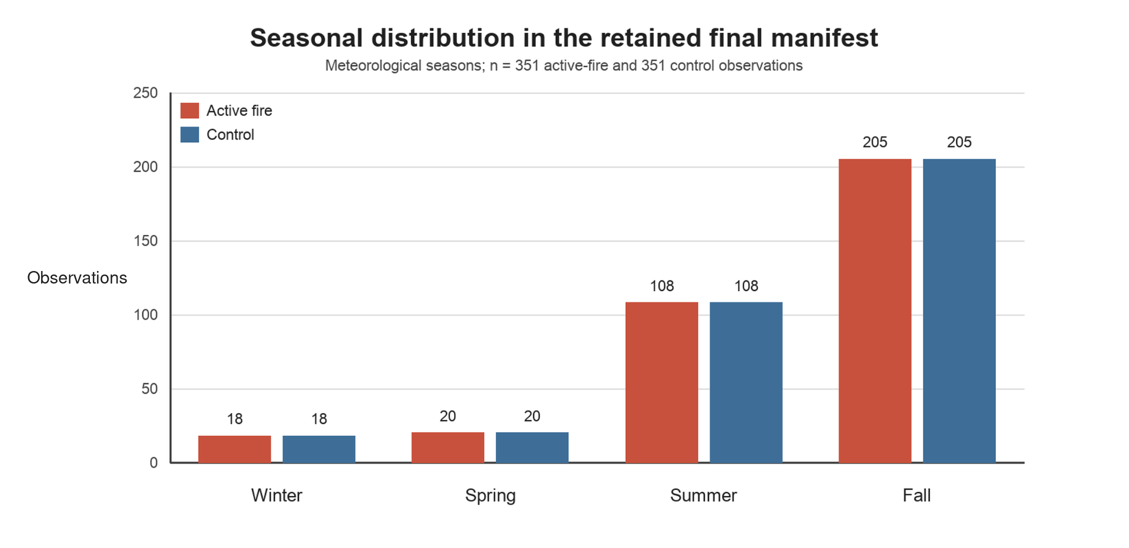
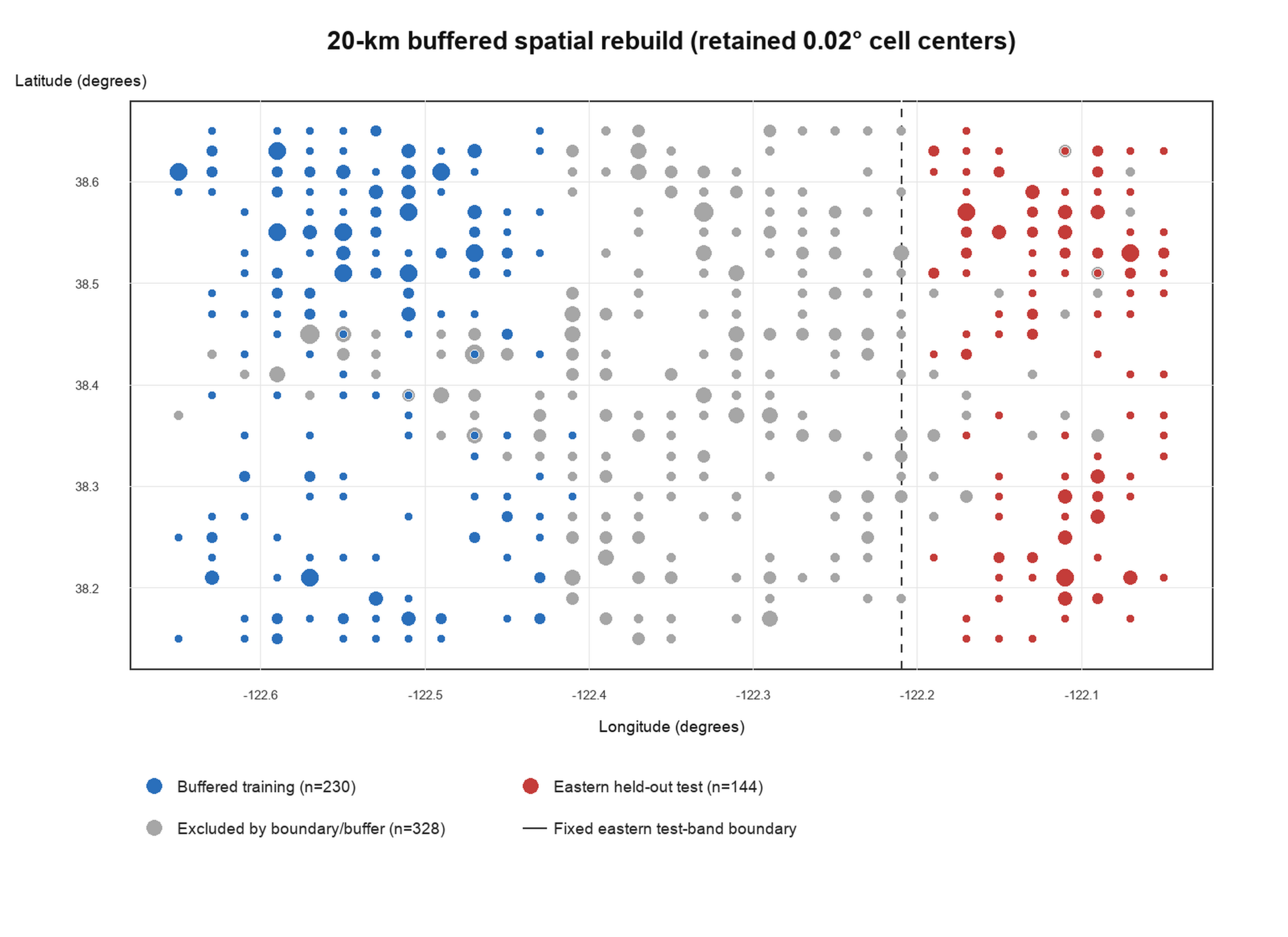
The final source manifest contains 702 observations: 351 recorded active-fire labels and 351 date-paired controls (Table 1). The observed retained acquisition-date span is 29 March 2001 through 2 March 2023. The original seed-42 cell-grouped split assigned 425 retained 0.02-degree coordinate-cell groups: 255 groups with 411 observations to training, 85 groups with 140 observations to validation, and 85 groups with 151 observations to test. The original test therefore contained a median of 1 observation per cell (range 1–6). For the spatial rebuild, the fixed eastern holdout and 20-km buffer retained 141 training cells with 230 observations (110 fire, 120 control) and 93 held-out test cells with 144 observations (50 fire, 94 control); 328 source observations were excluded by the boundary or buffer. The buffered test also had a median of 1 observation per cell (range 1–4), was not class-balanced, and has threshold metrics that are descriptive of that selected test set only. The manifest’s seasonal distribution is shown in Figure 1.

Cohort or partition	Fire	Control	Total
Full retained manifest	351	351	702
Buffered rebuild: training	110	120	230
Buffered rebuild: held-out test	50	94	144
Excluded by spatial boundary/buffer	191	137	328

Spatial Grouping and Overlap Audit

The released code defined a group as cell_floor(latitude/0.02)_floor(longitude/0.02): coordinates were floored, not rounded, into half-open 0.02-degree latitude and longitude cells. At Napa latitudes, a cell is approximately 2.22 km north-south by 1.74 km east-west. The original split was stratified by each group’s majority label and assigned approximately 60%/20%/20% of groups to train/validation/test using seed 42. Across that original split, distance from a test-cell center to its nearest development-cell center was 1.737 km at minimum, 1.743 km at median, and 4.143 km at maximum; all 85 original test groups lay within 5 km of a development group. Thus, the original grouping eliminated literal cell reuse but did not ensure nonoverlapping image chips or independent wildfire incidents. This audit motivated the rebuilt primary evaluation below.

Incident-Proxy Audit

Original coordinates and official incident identifiers were not retained, so a true official-incident count cannot be reconstructed. As an overlap warning for the original split, we linked retained positive date-cell records when cell centers were within 10 km and dates were within 7 days. This operational proxy formed 64 components; 9 crossed original partitions, including 6 spanning train, validation, and test. These components are not verified fire incidents, but they demonstrate why the original cell-grouped benchmark cannot rule out incident overlap.

Buffered Spatial Rebuild

We rebuilt the primary split from the retained cell manifest using the same 10-km/7-day positive incident-proxy rule. A fixed eastern test band (cell-center longitude at or east of -122.21) was chosen from geography and class counts, not imagery or model scores. A whole positive component entered the test set only when all of its cells lay in that band; components straddling the boundary were excluded rather than divided. We then excluded every non-test positive component touching a 20-km test buffer and every control within that buffer. Among the 64 positive incident-proxy components, 19 were retained in training, 19 were retained in test, and 26 were excluded by the geographic boundary or outer buffer; 0 crossed retained partitions. The resulting split retained 141 training cells and 93 test cells and had an observed minimum test-to-training cell-center separation of 20.334 km. This conservative center buffer exceeds the approximately 14.1-km requested chip-footprint diagonal plus uncertainty from retaining cells rather than original coordinates. Because a second buffered validation partition was infeasible in the retained regional sample, the refit used the unchanged architecture and a fixed 25 epochs, with no scheduler, early stopping, or validation-selected checkpoint. The resulting spatial split is shown in Figure 2.

Positive-Label Provenance and Audit

Positive labels were drawn from a preprocessed NASA FIRMS table restricted to longitude −122.65 to −122.05 and latitude 38.15 to 38.65. Released construction code standardized latitude, longitude, and acquisition date; removed rows with missing values and exact duplicate coordinate-date records; and sampled at most 351 positive records with seed 42. The raw input CSV and source metadata were not retained, so the original preselection count and each original row’s platform, NRT-versus-standard state, confidence, type, and quality fields cannot be recovered. We audited the 351 retained labels against the NASA FIRMS MODIS Collection 6.1 standard archive³¹. Linking by acquisition date and retained 0.02° cell, all 351 labels (304 unique date-cell combinations) had at least one standard-archive candidate, totaling 956 candidate detections. The audit accepted Terra or Aqua records and applied no confidence, type, or additional quality threshold; it establishes date-cell consistency, not a unique original-row match.

Date-Paired Control Construction

Released code generated one control for each sampled positive date. Candidate longitude and latitude were drawn independently and uniformly within the same bounding box; this is date pairing, not land-cover or terrain matching. A candidate was accepted only if its center was at least 5 km from every detection in the bounding-box-filtered input on that date (seed 42; at most 10,000 attempts); the code aborts rather than accepts a candidate if that cap is reached. The rerun read the first 351 controls. Per-control attempt counts and whether a run encountered the cap were not preserved, but the cap could not silently admit a failed candidate. The code did not check detections outside the box, enforce unique controls, or apply a multi-day exclusion. At retained-cell resolution, controls occupy 346 unique date-cell combinations; no date-cell occurs in both classes, while 83 cells occur in both classes on different dates. Control validation used the label date, whereas image retrieval selected an 8-day composite whose period could be offset by up to ±8 days; the effective imagery exposure window can therefore be wider than the same-date exclusion (approximately label−8 through label+15 days under the retrieval rule). Thus, the 5-km center rule did not guarantee that a control image contained no recorded fire. FIRMS point records contain detections only and carry no no-observation category; separating true no-fire from no-observation would require a gridded product such as MOD14A1, which was not used.

Image Construction and Temporal Alignment

Code queried Planetary Computer’s MOD09A1.061 collection, the MODIS/Terra 8-day Level-3 500-m surface-reflectance product³². For each retained label, code requested a ±0.05-degree longitude/latitude box, an approximately 11.1-km north-south by 8.7-km east-west footprint at the study latitude (about 14.1 km diagonally), and searched a ±8-day date window. The requested physical extent is distinct from the stored array size: each red (sur_refl_b01), green (sur_refl_b04), and blue (sur_refl_b03) channel originated at 500-m product resolution, and the extracted grid-aligned window was bilinearly resized to a stored 128 x 128 RGB PNG. Pixel-grid alignment can change the number of native edge samples, but not the stated requested geographic box. The catalog item closest to the label date was selected. Raw reflectance was multiplied by 0.0001, then each chip received a joint 2nd-98th-percentile stretch, clipping to 0-1; NaNs were set to zero. There was no explicit QA-band, cloud, missing-data, or smoke filter beyond the product’s own compositing and invalid-percentile rejection. The retained manifest/PNGs do not preserve the selected item ID, acquisition timestamp, or exact offset from each label date, so strict pre-event alignment cannot be reconstructed.

Negative-Rule Sensitivity Analysis

We re-filtered retained controls against the full standard archive, including detections outside the study-box edge, and recomputed held-out AUROC from saved predictions without retraining. Under this conservative cell-level full-archive re-audit, the same-day ≥5-km rule retained 330 of 351 controls: 21 (6.0%) did not satisfy the stronger audit condition. The original bounding-box-only check is a known source of label-eligibility uncertainty, but exact control coordinates and the original input table were not retained, so the 21 exclusions cannot all be attributed solely to outside-box detections. Distance was calculated as a lower bound from each retained 0.02° cell to the nearest archived detection; a control survived only when its entire cell satisfied the threshold. We evaluated same-date thresholds of 5, 10, and 20 km and 5-km windows of ±3 and ±7 days. The ±7-day, 5-km row partially tests the wider composite clock: its CNN AUROC was 0.941, but ±7 days does not cover the worst-case label−8 through label+15 composite span. A definitive assessment requires preserved per-chip item IDs and timestamps. For each reduced test subset, 95% CIs used 2,000 stratified bootstrap resamples. These nested analyses test proximity to recorded detections; they neither make controls landscape matched nor test a rebuilt spatial split.

Spatial-Buffer Sensitivity Analysis

We repeated the complete split construction and refitted both image models after increasing only the outer cell-center buffer from 20 to 30 km; the fixed eastern test band, 10-km/7-day incident-proxy rule, preprocessing, seed 42, and fixed 25-epoch training rule were unchanged. The held-out test therefore remained the same 144 observations (50 active-fire labels and 94 controls), while training decreased from 230 observations at 20 km to 82 at 30 km (19 active-fire labels and 63 controls). The 30-km split retained 9 positive proxy components in training and 19 in test, excluded 36 components, had 0 crossing components, and achieved a minimum observed test-to-training cell-center separation of 30.037 km. Because buffer size and available training sample size change together in this regional geometry, the comparison assesses robustness to a stricter separation protocol rather than a pure distance effect.

Multi-Seed Replication

We repeated both model fits with five independent seeds (7, 21, 42, 84, and 123) on each evaluation split: the original cell-grouped split, the 20-km buffered split, and the 30-km buffered split. Every replication used the identical fixed 25-epoch protocol with no validation-selected checkpoint. We report the mean, sample standard deviation, and range of test AUROC across seeds. Both models’ test probabilities, labels, row identifiers, and retained cell identifiers were saved for every seed to support paired downstream cell-cluster-bootstrap analysis.

Variables and Measurements

The binary target is the retained recorded-active-fire versus date-paired-control label. The input is the reconstructed RGB chip. Its full construction and temporal-alignment workflow is specified in the preceding Image Construction and Temporal Alignment subsection; Table 2 summarizes the common preprocessing applied before both models and each model’s subsequent configuration. ResNet-18 follows³³, and the Image RF follows the Random Forest framework³⁴.

Component	Verified implementation
Image source and chip	MOD09A1.061 MODIS/Terra 8-day, 500-m surface reflectance; RGB b01/b04/b03. Search: ±0.05° bbox and ±8 d from label; nearest catalog item. Stored 128 × 128 RGB PNG. Both models received the same retrieved PNGs and base preprocessing before their model-specific transforms.
Preprocessing and QC	Reflectance ×0.0001; joint per-chip 2nd–98th percentile stretch; clip 0–1; NaNs → 0; bilinear resize. Both models shared these steps; only model-specific transforms differed. No explicit QA-band, cloud, smoke, or missing-data filter beyond product compositing/invalid-percentile rejection.
CNN architecture/training	ImageNet-pretrained ResNet-18 with all layers fine-tuned; final 512-to-1 logit; BCEWithLogitsLoss; AdamW (lr 0.001; unspecified options used library defaults); batch 32; 25 epochs.
CNN transforms/selection	Train: resize 224 x 224, random horizontal/vertical flips, ImageNet normalization. Evaluation: resize + normalization only. Seed 42; deterministic cuDNN; no scheduler or early stopping. The original cell benchmark saved the best validation-AUROC checkpoint; the buffered rebuild used the same transforms but a fixed 25-epoch run with no validation-selected checkpoint.
Image RF	Frozen ImageNet ResNet-18 average-pool features (512 dimensions), then Random Forest: 400 trees, max_depth=None, random_state=42, n_jobs=−1, class_weight=balanced_subsample.

Procedure

We standardized retained FIRMS labels, generated date-paired controls, and used the released retrieval script to select the nearest available MOD09A1.061 catalog item within its search window and produce a 128 x 128 RGB PNG. For diagnostic comparison, we retain the original seed-42 0.02-degree cell-grouped benchmark. For the primary evaluation, we rebuilt the manifest before model fitting with the fixed eastern holdout, whole incident-proxy components, and 20-km outer buffer described above. The CNN used random horizontal and vertical flips during training; all images were resized to 224 x 224 and ImageNet-normalized. The spatial refit trained exactly 25 epochs and evaluated the held-out test set once; it did not choose a checkpoint from a nearby validation split.

Data Analysis

AUROC was the primary ranking metric; we also report Brier score³⁵, expected calibration error (ECE)³⁶, accuracy, F1, sensitivity, and specificity. Brier score is the mean squared error between a predicted probability and the binary label. ECE was calculated separately for each model and evaluation from uncalibrated test probabilities using 10 fixed, equal-width bins over [0, 1]; it is the sample-size-weighted absolute difference between mean predicted probability and observed active-fire-label frequency within each nonempty bin. CNN probabilities were sigmoid-transformed logits, and Image RF probabilities were the forest’s class-1 predict_proba outputs; no post-hoc calibration was applied. Accuracy, F1, sensitivity, and specificity were calculated at a fixed 0.50 probability threshold. This conventional, model-neutral cutoff was retained only as a descriptive reference, was not tuned on the held-out test set, and is not an operational wildfire-decision threshold. Because the source dataset was intentionally class-balanced and the buffered test is spatially selected rather than prevalence-representative, all threshold-dependent metrics do not describe operational performance.

Bootstrap Inference

Individual model AUROC confidence intervals in representative runs used 2,000 stratified observation-level resamples. Because these resamples treat observations within the same retained cell as independent, the Table 3 and Table 5 intervals can understate true sampling uncertainty when a cell contributes more than one test observation (median 1, range 1–6 in the original test and 1–4 in the buffered test); the cluster bootstrap described next addresses this dependence directly for the paired comparison. For the multi-seed paired comparison, each split and seed used a 10,000-draw nonparametric cell-cluster bootstrap: test cells were sampled with replacement, all observations in selected cells were retained, and CNN-minus-Image-RF AUROC was computed on the same sampled rows. Percentile intervals use the 2.5th and 97.5th percentiles. This handles repeated observations within retained cells but not dependence between nearby cells, retraining uncertainty, or external-landscape generalization.

Ethical Considerations

This study used publicly available NASA FIRMS labels and MODIS imagery and did not involve human participants, personally identifiable information, or private records. Therefore, institutional human-subject review and informed-consent procedures were not applicable.

Results

Performance of Verified Standalone Models

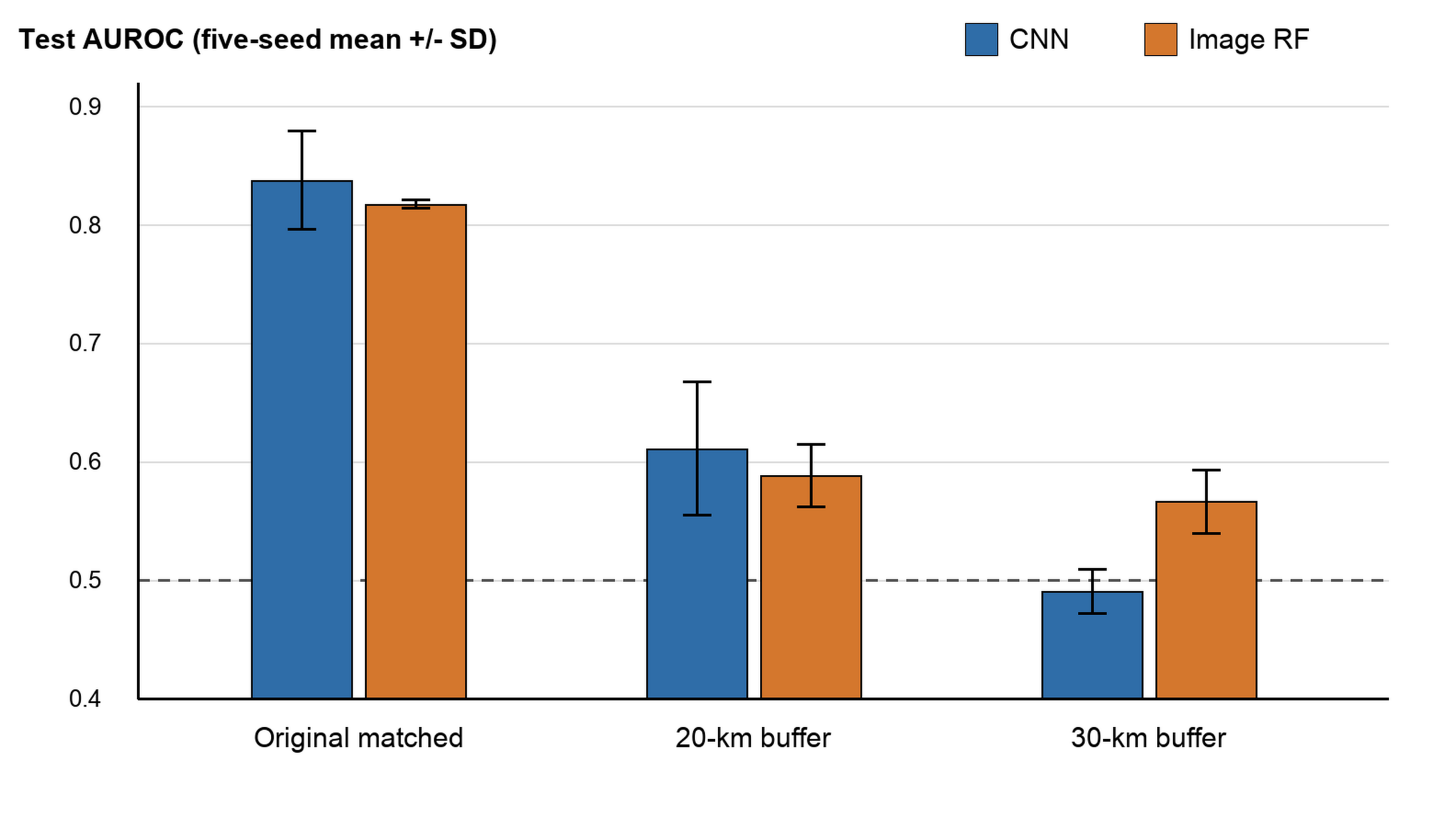
The originally reported seed-42 cell-grouped benchmark yielded CNN AUROC 0.920 (95% observation-level CI 0.874-0.958) and Image RF AUROC 0.816 (0.744-0.879). Under the matched fixed-25-epoch/no-checkpoint protocol, the same split produced five-seed means of 0.838 ± 0.042 for CNN (range 0.768-0.873) and 0.817 ± 0.003 for Image RF (0.813-0.821). The RF result was essentially unchanged, whereas the lower matched-protocol CNN mean shows that checkpoint selection contributed materially to the originally reported 0.920. Under geographic separation, mean AUROC declined for both models (Table 4; Figure 3), showing that the original cell-grouped scores do not establish spatially independent discrimination.

Paired and Clustered Robustness

For each split and seed, a 10,000-draw paired bootstrap resampled retained test cells with replacement and recomputed AUROC(CNN) minus AUROC(Image RF) on identical sampled observations. On the original split, differences for seeds 7, 21, 42, 84, and 123 were 0.047 (95% CI -0.035 to 0.129), 0.056 (-0.028 to 0.137), -0.048 (-0.127 to 0.035), 0.016 (-0.073 to 0.104), and 0.030 (-0.050 to 0.111), respectively. At 20 km they were 0.093 (-0.040 to 0.223), 0.028 (-0.096 to 0.158), 0.008 (-0.101 to 0.127), -0.045 (-0.172 to 0.087), and 0.030 (-0.116 to 0.178). At 30 km they were -0.077 (-0.217 to 0.061), -0.129 (-0.286 to 0.032), -0.089 (-0.241 to 0.071), -0.016 (-0.140 to 0.108), and -0.068 (-0.175 to 0.043). The mean paired differences were therefore 0.020, 0.023, and -0.076 across the three splits. Every seed-specific interval crossed zero, so the crossover in point estimates does not establish within-seed superiority.

Threshold and Calibration Interpretation

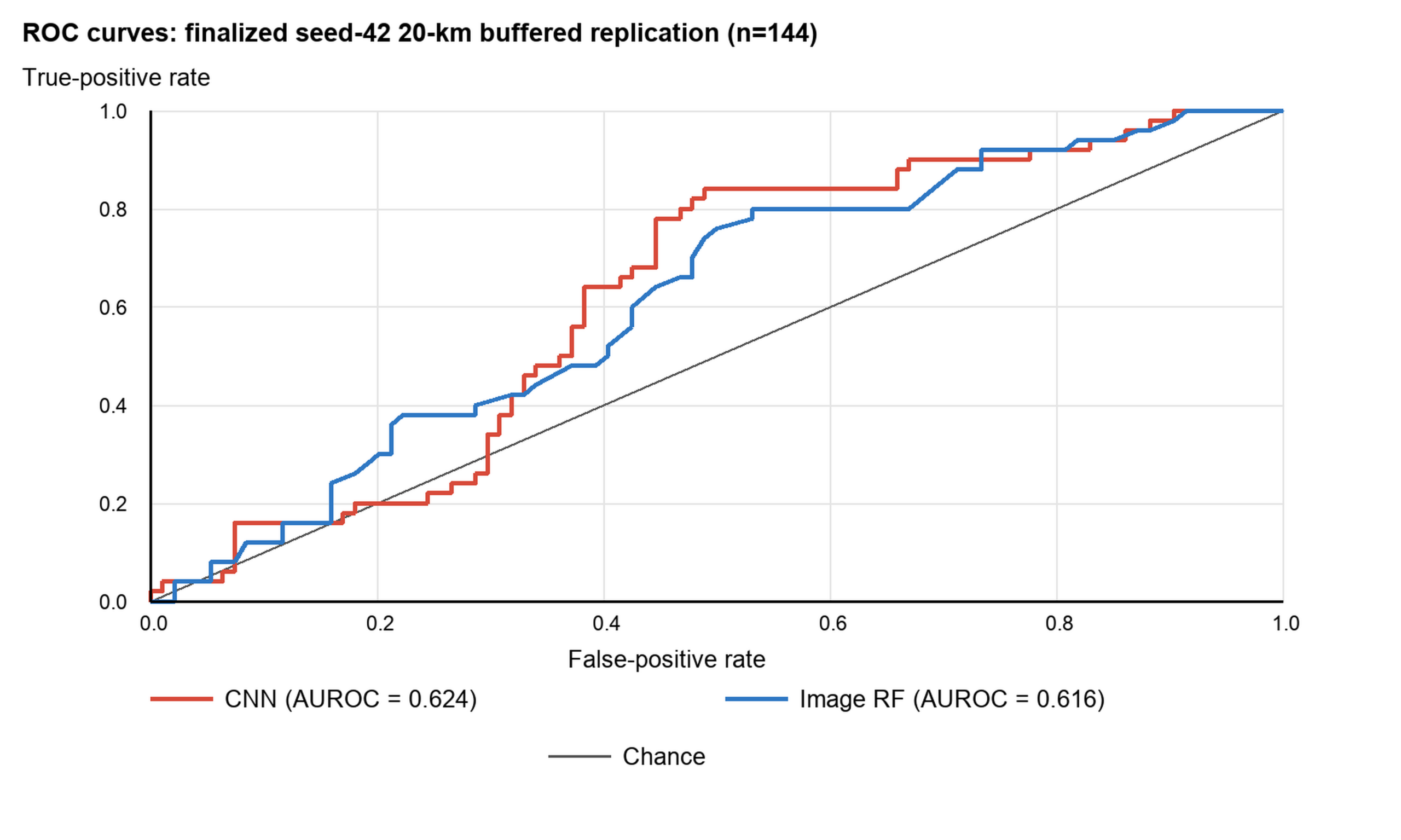
In the finalized seed-42 20-km replication, Image RF had a lower Brier score (0.222 versus 0.309) and ECE (0.071 versus 0.303) than CNN within this constructed test distribution. At the fixed 0.50 threshold, CNN sensitivity/specificity were 0.180/0.830 (9 of 50 active-fire labels detected), whereas Image RF sensitivity/specificity were 0.020/0.979 (1 of 50 detected). CNN accuracy was 0.604 and Image RF accuracy was 0.646, both below the 0.653 majority-control baseline; F1 values were 0.240 and 0.038, respectively. More importantly, across all five matched replications, Image RF sensitivity was 0.020 at 20 km and 0.000 at 30 km in every seed. Thus, its higher mean 30-km AUROC describes probability ranking across thresholds, not useful detection at the prespecified 0.50 cutoff. These calibration and threshold summaries remain descriptive and can change under real-world prevalence or a landscape-matched control set.

Evaluation / model	AUROC	95% CI	Brier	ECE	Accuracy	F1	Sens. / spec. (0.50)
Cell split, seed 42 / CNN	0.920	0.874–0.958	0.150	0.146	0.788	0.816	0.910 / 0.658
Cell split, seed 42 / Image RF	0.816	0.744–0.879	0.190	0.132	0.762	0.769	0.769 / 0.753
20-km buffer, seed 42 / CNN	0.624	0.528-0.716	0.309	0.303	0.604	0.240	0.180 / 0.830
20-km buffer, seed 42 / Image RF	0.616	0.519–0.709	0.222	0.071	0.646	0.038	0.020 / 0.979

Split	CNN AUROC	Image RF AUROC	Mean paired difference
Original	0.838 ± 0.042 (0.768-0.873)	0.817 ± 0.003 (0.813-0.821)	+0.020
20 km	0.611 ± 0.056 (0.513-0.655)	0.588 ± 0.026 (0.558-0.616)	+0.023
30 km	0.490 ± 0.019 (0.463-0.512)	0.566 ± 0.027 (0.528-0.593)	-0.076

Control-Definition Sensitivity: The archived-detection sensitivity analysis remains a post hoc re-filtering of predictions from the original retained cell-grouped test, not a test of the buffered refit. Across its nested same-day subsets, CNN AUROC increased from 0.920 in the original retained set to 0.923 (5 km), 0.945 (10 km), and 0.956 (20 km) (Table 5). One reading is that proximity to a recorded detection did not create the original score; an equally plausible reading is landscape-context confounding, because controls farther from detections may increasingly occupy different land-cover or terrain settings. These nested analyses cannot distinguish those explanations, and the much lower buffered results reinforce the need for land-cover-stratified or propensity-matched controls. The ±3- and ±7-day rules retained different numbers of controls overall (277 and 270) but the same 55 original-test controls; their identical test AUROCs are therefore by construction, not a copied value.

Spatial-Buffer Sensitivity

Across five seeds, the 20-km split produced CNN AUROC 0.611 ± 0.056 (range 0.513-0.655) and Image RF AUROC 0.588 ± 0.026 (0.558-0.616). On the unchanged eastern test set at 30 km, CNN AUROC was 0.490 ± 0.019 (0.463-0.512) and Image RF AUROC was 0.566 ± 0.027 (0.528-0.593). CNN therefore had the higher mean at 20 km, whereas Image RF had the higher mean at 30 km. The stricter buffer reduced training from 230 to 82 observations and from 19 to 9 training incident-proxy components, so distance and available training sample size changed together. The result is a conservative stress test, not a pure estimate of buffer distance.

Control exclusion rule	All controls	Test controls	CNN AUROC (95% CI)	Image RF AUROC (95% CI)
Original retained set	351	73	0.920 (0.874–0.958)	0.816 (0.744–0.879)
Standard archive: same day, ≥5 km	330	67	0.923 (0.878–0.959)	0.815 (0.742–0.882)
Standard archive: same day, ≥10 km	247	54	0.945 (0.909–0.975)	0.834 (0.756–0.902)
Standard archive: same day, ≥20 km	147	31	0.956 (0.917–0.984)	0.842 (0.759–0.918)
Standard archive: ±3 days, ≥5 km	277	55	0.941 (0.903–0.975)	0.852 (0.781–0.912)
Standard archive: ±7 days, ≥5 km	270	55	0.941 (0.903–0.975)	0.852 (0.781–0.912)

Excluded Extensions

We did not include LSTM³⁷ or TCN³⁸ benchmarks because the retained dataset does not contain repeated, closely spaced pre-event observations at fixed sites; a sequence model built on the current date-associated composite would retain the same temporal-alignment and control-construction limitations and should be evaluated with an incident-aware spatial buffer. For the same reproducibility reason, we withhold feature-importance analysis for Proxy RF and an ensemble of the two models until their tabular inputs, predictions, and validation/test alignment are reproducible; an ensemble’s weights should be chosen on validation data and evaluated once on the held-out test set.

Discussion

Summary of Findings and Methodological Boundaries

Model comparison was buffer-distance-dependent rather than a blanket win for either approach. Under the matched fixed-25-epoch protocol, CNN mean AUROC exceeded Image RF on the original cell split (0.838 versus 0.817) and at 20 km (0.611 versus 0.588), but Image RF overtook CNN at 30 km (0.566 versus 0.490). One plausible explanation is that the RF’s frozen, spatially averaged ImageNet features preserve probability ordering more consistently than a fully fine-tuned CNN as geographic separation increases and the available training set shrinks; the present design cannot separate those mechanisms. Because the negative samples were constructed rather than naturally observed, some discrimination may reflect differences introduced by the sampling procedure rather than generalizable wildfire-related visual features; accordingly, AUROC is not a direct measure of real-world wildfire-prediction ability. This ranking result must not be read as practical fire-detection superiority: at the 0.50 threshold, Image RF sensitivity was 0.020 at 20 km and 0.000 at 30 km for every seed. Moreover, every seed-specific paired cell-cluster-bootstrap interval crossed zero, so the AUROC point-estimate rankings do not establish model superiority. The matched-protocol original CNN mean also fell well below the validation-checkpoint-selected 0.920, demonstrating sensitivity to model-selection protocol in addition to spatial design. The broader conclusion remains unchanged: nearby cells and crossing incident-proxy components make the original high AUROC insufficient evidence of spatially independent discrimination. Residual east-west distribution shift, near-event imagery, and unmatched landscape context further limit interpretation, and neither model estimates prospective wildfire risk.

Directions for Future Research

Next work should preserve original coordinates, official incident identifiers, source-product metadata, selected item IDs, and timestamps; repeat buffered evaluation over multiple geographic holdouts, buffer distances, and an external landscape; and use strictly pre-event imagery and predictors. The present 30-km stress test supports the 20-km interpretation but also shows that larger buffers rapidly reduce the available training sample in this small regional dataset. A prospective study should therefore predefine buffer scales using chip geometry, recruit enough independent incidents to sustain each scale, match or stratify controls by land cover and terrain (or use propensity matching), report target availability and quality masks, and assess whether any remaining performance persists under those conditions.

Acknowledgments

The author thanks Dr. Fa Li, Assistant Professor in the Department of Earth and Planetary Sciences at the Jackson School of Geosciences, The University of Texas at Austin, for guidance on this independent research work.

Data and Code Availability

The original code and retained source artifacts are publicly available at https://www.kaggle.com/datasets/coolrhea/microwildfirev2-source. During review, a reproducibility package containing the source and buffered split manifests, rebuild notebook, regenerated figures/tables, provenance and control-sensitivity audits, software environment, and detailed reconstruction instructions is available to editors on request; a permanent public archive will be released on acceptance. Five-seed artifacts for all three splits include per-seed CNN and Image RF test predictions, labels, row and cell identifiers, metric summaries, split audits, and the paired cell-cluster-bootstrap calculation. Full image chips are not redistributed; they can be regenerated from public sources under the documented procedure. Because original coordinates and per-chip item IDs were not retained, the package verifies the reported retained-cell analysis rather than reproducing the original PNG collection byte-for-byte.

Acknowledgments

The author thanks Dr. Fa Li, Assistant Professor in the Department of Earth and Planetary Sciences at the Jackson School of Geosciences, The University of Texas at Austin, for reviewing and commenting on a draft of this manuscript. The research was conceived, conducted, and written independently.

References

1. L. Giglio, J. Descloitres, C. O. Justice, and Y. J. Kaufman. An enhanced contextual fire detection algorithm for MODIS. Remote Sensing of Environment. Vol. 87, pg. 273–282, 2003, https://doi.org/10.1016/S0034-4257(03)00184-6. [↩]
2. L. Giglio, W. Schroeder, and C. O. Justice. The collection 6 MODIS active fire detection algorithm and fire products. Remote Sensing of Environment. Vol. 178, pg. 31–41, 2016, https://doi.org/10.1016/j.rse.2016.02.054. [↩] [↩]
3. F. Huot, R. L. Hu, N. Goyal, T. Sankar, M. Ihme, and Y. F. Chen. Next day wildfire spread: a machine learning dataset to predict wildfire spreading from remote-sensing data. IEEE Transactions on Geoscience and Remote Sensing. Vol. 60, pg. 1–13, 2022, https://doi.org/10.1109/TGRS.2022.3192974. [↩]
4. P. Jain, S. C. P. Coogan, S. G. Subramanian, M. Crowley, S. Taylor, and M. D. Flannigan. A review of machine learning applications in wildfire science and management. Environmental Reviews. Vol. 28, pg. 478–505, 2020, https://doi.org/10.1139/er-2020-0019. [↩]
5. A. Trucchia, H. Izadgoshasb, S. Isnardi, P. Fiorucci, and M. Tonini. Machine-learning applications in geosciences: comparison of different algorithms and vegetation classes’ importance ranking in wildfire susceptibility. Geosciences. Vol. 12, art. 424, 2022, https://doi.org/10.3390/geosciences12110424. [↩]
6. M. Rodrigues and J. de la Riva. An insight into machine-learning algorithms to model human-caused wildfire occurrence. Environmental Modelling & Software. Vol. 57, pg. 192–201, 2014, https://doi.org/10.1016/j.envsoft.2014.03.003. [↩]
7. F. Guo, L. Zhang, S. Jin, M. Tigabu, Z. Su, and W. Wang. Modeling anthropogenic fire occurrence in the boreal forest of China using logistic regression and random forests. Forests. Vol. 7, art. 250, 2016, https://doi.org/10.3390/f7110250. [↩]
8. K. N. Babu, R. Gour, K. Ayushi, N. Ayyappan, and N. Parthasarathy. Environmental drivers and spatial prediction of forest fires in the Western Ghats biodiversity hotspot, India: an ensemble machine learning approach. Forest Ecology and Management. Vol. 540, art. 121057, 2023, https://doi.org/10.1016/j.foreco.2023.121057. [↩]
9. S. Milanovic, J. Kaczmarowski, M. Ciesielski, Z. Trailovic, M. Mielcarek, R. Szczygiel, M. Kwiatkowski, R. Balazy, M. Zasada, and S. D. Milanovic. Modeling and mapping forest fire occurrence in Lower Silesian, Poland. Forests. Vol. 14, art. 46, 2023, https://doi.org/10.3390/f14010046. [↩]
10. A. L. Achu, J. Thomas, C. D. Aju, G. Gopinath, S. Kumar, and R. Reghunath. Machine-learning modelling of fire susceptibility in a forest-agriculture mosaic landscape of southern India. Ecological Informatics. Vol. 64, art. 101348, 2021, https://doi.org/10.1016/j.ecoinf.2021.101348. [↩]
11. L. K. Sharma, R. Gupta, and N. Fatima. Assessing the predictive efficacy of six machine learning algorithms for wildfire susceptibility mapping. International Journal of Wildland Fire. Vol. 31, pg. 735–758, 2022, https://doi.org/10.1071/WF22016. [↩]
12. T. X. Truong, V.-H. Nhu, D. T. N. Phuong, L. T. Nghi, N. N. Hung, P. V. Hoa, and D. T. Bui. A new approach based on TensorFlow deep neural networks with Adam optimizer and GIS for spatial prediction of forest fire danger in tropical areas. Remote Sensing. Vol. 15, art. 3458, 2023, https://doi.org/10.3390/rs15143458. [↩]
13. N. Phelps and D. G. Woolford. Comparing calibrated statistical and machine learning methods for wildland fire occurrence prediction: a case study of human-caused fires in Lac La Biche, Alberta, Canada. International Journal of Wildland Fire. Vol. 30, pg. 850–870, 2021, https://doi.org/10.1071/WF20139. [↩]
14. G. Zhang, M. Wang, and K. Liu. Forest fire susceptibility modeling using a convolutional neural network for Yunnan province of China. International Journal of Disaster Risk Science. Vol. 10, pg. 386–403, 2019, https://doi.org/10.1007/s13753-019-00233-1. [↩]
15. S. Moghim and M. Mehrabi. Wildfire assessment using machine learning algorithms in different regions. Fire Ecology. Vol. 20, art. 104, 2024, https://doi.org/10.1186/s42408-024-00335-2. [↩]
16. K. Gholamnia, T. G. Nachappa, O. Ghorbanzadeh, and T. Blaschke. Comparisons of machine learning models for wildfire susceptibility mapping. Symmetry. Vol. 12, art. 604, 2020, https://doi.org/10.3390/sym12040604. [↩]
17. B. T. Pham, A. Jaafari, M. Avand, N. Al-Ansari, T. D. Du, H. P. H. Yen, T. V. Phong, D. H. Nguyen, H. Van Le, D. Mafi-Gholami, I. Prakash, H. T. Thuy, and T. T. Tuyen. Performance evaluation of machine learning methods for forest fire modeling and prediction. Symmetry. Vol. 12, art. 1022, 2020, https://doi.org/10.3390/sym12061022. [↩]
18. S. K. M. Abujayyab, M. M. Kassem, A. A. Khan, R. Wazirali, M. Coşkun, E. Taşoğlu, A. Öztürk, and F. Toprak. Wildfire susceptibility mapping using five boosting machine learning algorithms: the case study of the Mediterranean region of Turkey. Advances in Civil Engineering. Vol. 2022, art. 3959150, 2022, https://doi.org/10.1155/2022/3959150. [↩]
19. H. Moayedi, M. Mehrabi, D. T. Bui, B. Pradhan, and L. K. Foong. Fuzzy-metaheuristic ensembles for spatial assessment of forest fire susceptibility. Journal of Environmental Management. Vol. 260, art. 109867, 2020, https://doi.org/10.1016/j.jenvman.2019.109867. [↩]
20. A. Bjånes, R. De La Fuente, and P. Mena. A deep learning ensemble model for wildfire susceptibility mapping. Ecological Informatics. Vol. 65, art. 101397, 2021, https://doi.org/10.1016/j.ecoinf.2021.101397. [↩]
21. Q. He, Z. Jiang, M. Wang, and K. Liu. Landslide and wildfire susceptibility assessment in Southeast Asia using ensemble machine learning. Remote Sensing. Vol. 13, art. 1572, 2021, https://doi.org/10.3390/rs13081572. [↩]
22. V. C. Radeloff, D. P. Helmers, H. A. Kramer, M. H. Mockrin, P. M. Alexandre, A. Bar-Massada, V. Butsic, T. Hawbaker, S. Martinuzzi, A. D. Syphard, and S. I. Stewart. Rapid growth of the US wildland-urban interface raises wildfire risk. Proceedings of the National Academy of Sciences. Vol. 115, pg. 3314–3319, 2018, https://doi.org/10.1073/pnas.1718850115. [↩]
23. O. Ghorbanzadeh, K. Valizadeh Kamran, T. Blaschke, J. Aryal, A. Naboureh, J. Einali, and J. Bian. Spatial prediction of wildfire susceptibility using machine learning. Fire. Vol. 2, art. 43, 2019, https://doi.org/10.3390/fire2030043. [↩]
24. A. Al Saim and M. H. Aly. Machine learning for modeling wildfire susceptibility at state level: Arkansas, USA. Geographies. Vol. 2, pg. 31–47, 2022, https://doi.org/10.3390/geographies2010004. [↩]
25. S. Tavakkoli Piralilou, G. Einali, O. Ghorbanzadeh, T. Gudiyangada Nachappa, K. Gholamnia, T. Blaschke, and P. Ghamisi. A Google Earth Engine approach for wildfire susceptibility prediction fusion with remote sensing data of different spatial resolutions. Remote Sensing. Vol. 14, art. 672, 2022, https://doi.org/10.3390/rs14030672. [↩]
26. S. D. Chicas, J. Ø. Nielsen, M. C. Valdez, and C.-F. Chen. Modelling wildfire susceptibility in Belize’s ecosystems and protected areas using machine learning and knowledge-based methods. Geocarto International. Vol. 37, pg. 15823–15846, 2022, https://doi.org/10.1080/10106049.2022.2102231. [↩]
27. M. Rihan, A. A. Bindajam, S. Talukdar, Shahfahad, M. W. Naikoo, J. Mallick, and A. Rahman. Forest fire susceptibility mapping with sensitivity and uncertainty analysis using machine learning and deep learning. Advances in Space Research. Vol. 72, pg. 426–443, 2023, https://doi.org/10.1016/j.asr.2023.03.026. [↩]
28. Z. Shirazi, L. Wang, and V. G. Bondur. Modeling conditions appropriate for wildfire in Southeast China: a machine learning approach. Frontiers in Earth Science. Vol. 9, art. 622307, 2021, https://doi.org/10.3389/feart.2021.622307. [↩]
29. M. Naderpour, H. M. Rizeei, and F. Ramezani. Forest fire risk prediction: a spatial deep neural network-based framework. Remote Sensing. Vol. 13, art. 2513, 2021, https://doi.org/10.3390/rs13132513. [↩]
30. A. Malik, M. R. Rao, N. Puppala, P. Koouri, V. A. K. Thota, Q. Liu, S. Chiao, and J. Gao. Data-driven wildfire risk prediction in Northern California. Atmosphere. Vol. 12, art. 109, 2021, https://doi.org/10.3390/atmos12010109. [↩]
31. NASA Fire Information for Resource Management System (FIRMS). MODIS Collection 6.1 standard active-fire archive. https://firms.modaps.eosdis.nasa.gov/download/, accessed August 30, 2026. [↩] [↩]
32. E. Vermote. MODIS/Terra Surface Reflectance 8-Day L3 Global 500m SIN Grid V061 [Data set]. NASA EOSDIS Land Processes DAAC, 2021, https://doi.org/10.5067/MODIS/MOD09A1.061. [↩]
33. K. He, X. Zhang, S. Ren, and J. Sun. Deep residual learning for image recognition. Proceedings of CVPR. pg. 770–778, 2016, https://doi.org/10.1109/CVPR.2016.90. [↩]
34. L. Breiman. Random forests. Machine Learning. Vol. 45, pg. 5–32, 2001, https://doi.org/10.1023/A:1010933404324. [↩]
35. G. W. Brier. Verification of forecasts expressed in terms of probability. Monthly Weather Review. Vol. 78, pg. 1–3, 1950, https://doi.org/10.1175/1520-0493(1950)078<0001:VOFEIT>2.0.CO;2. [↩]
36. C. Guo, G. Pleiss, Y. Sun, and K. Q. Weinberger. On calibration of modern neural networks. Proceedings of the 34th International Conference on Machine Learning. pg. 1321–1330, 2017. [↩]
37. S. Hochreiter and J. Schmidhuber. Long short-term memory. Neural Computation. Vol. 9, pg. 1735–1780, 1997, https://doi.org/10.1162/neco.1997.9.8.1735. [↩]
38. S. Bai, J. Z. Kolter, and V. Koltun. An empirical evaluation of generic convolutional and recurrent networks for sequence modeling. arXiv:1803.01271, 2018, https://doi.org/10.48550/arXiv.1803.01271. [↩]