NHSJS

Double Pendulum Chaos in Uniform, Gradient, and Black-Hole Gravity

October 4, 2026

Abstract

The double pendulum is one of the simplest mechanical systems which exhibits chaotic motion and almost all the previous research assumes that the gravitational field is constant and uniform. The effect of modification of the gravitational field model on the onset of chaos and its amplitude of an ideal planar double pendulum is studied. Three gravity models were tested under same mechanical parameters and initial conditions – uniform gravity, a linear vertical gradient and a pseudo-Newtonian black-hole potential of the Paczyński-Wiita form. Ensemble Poincaré projections and finite-time Lyapunov exponents (FTLEs) were used to identify chaos in three regimes of initial conditions (regular, mixed, chaotic). Other parameter sweeps were done for different link-length ratios, mass ratios, and gravity-gradients. The dimensionless FTLE was decreased significantly from 0.0793 to 0.0213 in the chaotic regime by the use of the linear gradient model compared to the uniform gravity model. This suppression was found to not be monotonic, with the most chaotic flow occurring at a negative gradient and the least at a gradient of about dg/dy = +0.5 ms^-2m^-1 when using parameter sweeps. The pseudo-Newtonian model was very sensitive to the ratio of the link length to the pivot distance. Dynamics were very similar for the pivot far from the central mass (Configurations II and III). For the case where the pivot was near the Schwarzschild radius (Configuration I (ε ≈ 11.27) case), the quasi-periodic motion dominated and the value of the FTLE was close to 10⁻³. The results obtained indicate that the geometry of the gravitational field is an underutilized control parameter of chaos in mechanical coupled systems.

Keywords: double pendulum; chaos; Lyapunov exponent; Poincaré section; nonuniform gravity; Paczyński-Wiita potential; Hamiltonian dynamics

Introduction

However, chaos is a fundamental property of many physical systems, including phenomena which are extremely sensitive to the initial conditions and seem to be unpredictable on long time scales even if they are described by completely deterministic equations¹,². Small variations in initial conditions can quickly multiply, and in practice, it is impossible to predict the behavior of a system over a long period of time. The pioneering work of Lorenz demonstrated that this type of sensitive unpredictable behavior could be observed in simple low-dimensional systems, and forever altered the thinking of scientists about determinism and predictability in nature³. Since then chaos has been known to exist in many physical, biological and engineering systems and the understanding of what factors determine the level of chaos in a system has emerged as a major research objective².

One of the most widely studied chaotic systems in classical mechanics is the double pendulum: two rigid links connected end to end, free to swing in a plane under the influence of gravity⁴,⁵. Although the double pendulum is governed by simple Newtonian equations of motion obtained from Lagrangian mechanics, it can have a variety of behaviors, from regular, periodic oscillations to complete chaos in its trajectory, depending on its initial conditions and physical parameters, including the mass⁴ and length of the links. It is a relatively simple mechanical system which serves as a good paradigm for the study of chaos, and it has been studied in both classroom examples and research experiments.⁶

Tools of nonlinear dynamics are used to study and quantify chaos. One of the most important of these tools is the ensemble Poincaré plots: They are used to store the state of the system at every time it crosses a specified surface in phase space, transforming the continuous dynamics into a discrete map, which is easier to visualize⁷,⁸. The Poincaré section reveals smooth closed curves in the case of regular and periodic motion, and, in the case of chaotic motion, the points are distributed without order throughout a region of phase space. Another quantitative measure is the Lyapunov exponent which measures the exponential separation of neighboring trajectories in phase space with time⁹. The distinguishing characteristic of chaos is a positive Lyapunov exponent: Given two initially nearby trajectories, they will ultimately become completely uncorrelated.¹⁰ A convenient way to compute this measure of divergence is to use finite-time Lyapunov exponents (FTLEs) computed over a specific period of time, which is suitable for computational simulations that cannot be run to infinite time⁹,¹¹. Throughout the rest of the paper, $\lambda$ denotes the FTLE (1/s) and $\lambda^*$ its dimensionless form ( $\lambda^* = \lambda / \sqrt{g_{\mathrm{ref}} / L_1}$ ).

The double pendulum is part of the family of non-integrable Hamiltonian systems with conservative dynamics¹²,¹³. The Kolmogorov-Arnold-Moser (KAM) theorem states that the phase space of such systems is neither completely regular nor completely chaotic, but rather a complicated combination of stable regular islands and surrounding chaotic seas, where the proportion of the regular islands depends on the energy and parameters of the system⁸,¹⁴. It is not difficult to understand this mixed structure in case of the standard double pendulum in a uniform gravitational field for which the potential energy is just the potential energy of the vertical position of each mass⁴,⁵. Note that in this work we are only referring to KAM in a qualitative manner; quantitative KAM diagnostics (resonance overlap, invariant tori, frequency analysis) are not included and are left as future work¹⁵.

Most investigations of double pendulum chaos, to date, have been based on a homogeneous and uniform gravitational field.⁴,⁵,⁶ But, in many, physically interesting, scenarios gravity is not a uniform force. In the vicinity of large astronomical objects, however, there are spatial gradients that result in gravity varying across the length scales of an extended mechanical system¹⁶,¹⁷. In the regime of very short distances, as in the vicinity of near compact objects like neutron stars or black holes, gravity’s behavior is drastically different¹⁸. The Paczyński-Wiita pseudo-Newtonian potential was tailored specifically to achieve the essential aspects of the gravitational field of a Schwarzschild BH, including the radius of the innermost stable circular orbit and the qualitative nature of the strong-field dynamics, in a classical, Newtonian context, without necessitating a full general relativistic calculation. The potential has been extensively exploited in astrophysical fluid and orbit studies to study the effect of a strong and concentrated central gravity on the dynamical behavior¹⁹.

Although the double pendulum is frequently used as a model chaotic system, to our knowledge there has been no systematic study of how the strength, onset, and structure of the chaos in the double pendulum change as a function of the gravity field model used, especially one in which the gravity field is not uniform. Whether a linear vertical gravity gradient dampens or amplifies chaos, or whether the gravity of a pseudo-Newtonian black hole fundamentally changes the dynamics is unknown, as is whether it turns into nearly uniform dynamics when the pendulum is positioned far from the central mass. With a literature search conducted on Web of Science, Scopus and Google Scholar, we found the following recent studies that might be relevant to the present study: double-pendulum studies with magnetic forcing²⁰,²¹ and pseudo-Newtonian potentials applied to compact-object dynamics²²,²³, but not to the gravity-field-geometry effect on double-pendulum chaos.

In this work we aim to overcome this by simulating a planar ideal double pendulum in the presence of three gravity models: uniform gravity, linear vertical gradient and the Paczyński-Wiita pseudo-Newtonian potential using the Configurations I, II and III. Under each model, ensemble Poincaré projections and FTLEs were calculated for three typical initial-condition states (regular, mixed, chaotic) and parameter sweeps were performed to explore how the chaos intensity is influenced by the link-length ratio, mass ratio and gravity-gradient strength. Numerical integration was performed with the high-order DOP853 explicit Runge-Kutta method²⁴ from the SciPy scientific computing library²⁵. The authors demonstrate here that gravity field geometry is an underappreciated parameter for the chaos in coupled mechanical systems and they wed gravity field geometry to more exotic gravitational environments with the familiar textbook double pendulum.

Methods

Computational model

We simulated an ideal planar double pendulum consisting of two point masses ( $m_1$ , $m_2$ ) connected by massless rigid links ( $L_1$ , $L_2$ ) with a fixed pivot. Generalized coordinates were $q = [\theta_1, \theta_2]$ , where $\theta_1$ is the absolute angle of the first link from the vertical and $\theta_2$ is the relative angle of the second link with respect to the first (so the absolute second-link angle is $\theta_1 + \theta_2$ ). The state vector was $y = [\theta_1, \theta_2, \dot{\theta}_1, \dot{\theta}_2]$ .

The equations of motion were implemented in standard manipulator form:

M(q)\,\ddot{q} + H(q,\dot{q}) + \frac{\partial U(q)}{\partial q} = 0.

Here, $M(q)$ is the $2\times 2$ mass matrix, $H(q,\dot{q})$ collects Coriolis and centrifugal terms, and $U(q)$ is the potential energy. For all models, $M(q)$ and $H(q,\dot{q})$ were derived from the kinetic energy of point masses at the link ends; only the potential term $U(q)$ was changed to represent different gravity fields.

Gravity field models

The following three gravity models were tested with the same mechanical parameters and initial conditions (unless otherwise noted):

Uniform gravity (uniform_g). A constant downward gravitational force $g_0$ , which is provided by the potential energy $U = m_1 g_0 y_1 + m_2 g_0 y_2$ , where $y_1$ and $y_2$ are the vertical coordinates of the two masses.

Linear vertical gradient (linear_y). A position-dependent vertical gravity $g(y) = g_0(1 + \beta y / y_{\mathrm{ref}})$ , implemented by a per-unit-mass potential $\varphi(y) = g_0(y + 0.5\,\beta\,y^2/y_{\mathrm{ref}})$ , so that $\mathrm{d}\varphi/\mathrm{d}y = g(y)$ . The configuration used $\beta = 0.35$ and $y_{\mathrm{ref}} = 2.0$ m, equivalent to a gradient $\mathrm{d}g/\mathrm{d}y = g_0\,\beta/y_{\mathrm{ref}} = 1.71675\ \mathrm{m\,s^{-2}\,m^{-1}}$ . For the sake of analytical simplicity, this form was selected as the simplest non-uniform field analytically tractable; other choices ( $1/r$ Newtonian potential, radial-quadratic gradient) are reserved for future work.

Pseudo-Newtonian central potential (bh_pw). A central field potential centered at the origin of the form Paczyński–Wiita potential $\varphi(r) = -\mu/(r - r_s)$ , where $r = |\mathbf{r}|$ and $r_s$ is a length parameter¹⁹,²²,²³. We assume $\mu$ and $r_s$ are independent and equivalent to the two dimensionless ratios $\varepsilon = L_1/R_{\mathrm{pivot}}$ and $k = R_{\mathrm{pivot}}/r_s$ . The pivot was made at point $y$ -axis at a distance $R_{\mathrm{pivot}}$ from the origin. Potential energy was $U = m_1\,\varphi(|\mathbf{r}1|) + m_2\,\varphi(|\mathbf{r}_2|)$ with $\mathrm{d}\varphi/\mathrm{d}r = \mu/(r - r_s)^2$ . The value of the coefficient $\mu$ was chosen such that the local acceleration at the pivot equals the target acceleration $g{\mathrm{target}} = 9.81\ \mathrm{m\,s^{-2}}$ , i.e. $\mu = g_{\mathrm{target}}(R_{\mathrm{pivot}} - r_s)^2$ . Three configurations were tested at $k = 10$ : Configuration I ( $\varepsilon \approx 11.27$ ), Configuration II ( $\varepsilon \approx 3.39 \times 10^{-5}$ ), and Configuration III ( $\varepsilon \approx 7.88 \times 10^{-12}$ ). These values of $\varepsilon$ would be the Schwarzschild radii of black holes from planetary to supermassive masses at $k = 10$ , but the dynamics is not a function of mass, it is a function of $\varepsilon$ so we report it by $\varepsilon$ .

Potential gradients and generalized gravity torques

For uniform_g and linear_y models, the gravity contribution was computed from the vertical positions $y_1(q)$ and $y_2(q)$ and the derivative $\mathrm{d}\varphi/\mathrm{d}y$ via the chain rule.

For the bh_pw model, gravity depends on the radial distance from the central mass. Let $\mathbf{r}_k(q)$ be the Cartesian position of bob $k$ and $s_k = |\mathbf{r}_k|$ . The potential energy is $U(q) = \sum_k m_k\,\varphi(s_k)$ . The generalized gravity terms were computed by:

\frac{\partial U}{\partial \theta_i} = \sum_k m_k \frac{\mathrm{d}\varphi}{\mathrm{d}r}(s_k) \cdot \frac{\mathbf{r}_k \cdot \partial \mathbf{r}_k/\partial \theta_i}{s_k}, \qquad i \in \{1,2\}.

The derivatives $\partial \mathbf{r}_k/\partial \theta_i$ were computed analytically from the link geometry, enabling a direct evaluation of $\partial U/\partial q$ at each time step.

Numerical integration and stability controls

The time integration employed a high order explicit Runge-Kutta method (DOP853) together with the event detection provided by the SciPy solve_ivp routine. The absolute and relative tolerances were atol = 1e-12 and rtol = 1e-10. The nominal maximum time step was max_step = 0.015 s. Percent drift was tracked for each run as energy conserved was monitored by comparing the total mechanical energy of the system $E(t) = T(t) + U(t)$ at the start and end of the trajectory. DOP853 is not a symplectic integrator, but for our tolerances and 60 s horizon, the measured energy drift remained below $10^{-8}$ % for all runs (see Results § “Sampling quality” for info on the drift values). It was decided to test a symplectic integrator with fixed step size $h = 0.005$ s that uses an implicit-midpoint method, on the same IC as the canonical chaotic one, and a similar run with max $|\mathrm{drift}| \approx 4.4 \times 10^{-2}$ % was performed, which is about five million times larger than the result from the DOP853 integrator. To check the sensitivity of the FTLE values, max_step was reduced by a factor of 2, or atol = 1e-13, rtol = 1e-11, with the canonical chaotic IC, showing a change in $\lambda^*$ of less than 0.001%.

Base simulations used $t \in [0.0,\ 120.0]$ s. To minimise missed crossings, the window of integration $t$ was scaled up to $[0.0,\ 300.0]$ s and section_max_step was set to 0.04 s for Poincaré sampling. A smaller integration step max_step = 0.012 s) and a shorter integration horizon (t_span = [0, 90] s) were used for bh_pw, while a smaller section step section_max_step = 0.03 s) and a shorter section horizon (section_t_span = [0, 220] s) were used.

In the case of bh_pw, an extra terminal safety event terminated the integration, if either mass reached $r \leq r_s + 0.5 \cdot \min(L_1, L_2)$ due to the resulting numerical instability from the divergence of $\varphi(r)$ at $r_s$ .

Chaos diagnostics

Poincaré sections were constructed by recording the state when the first link crossed the section $\theta_1 \equiv 0\ \mathrm{mod}\ 2\pi$ . Crossings were detected via the root of $\sin(\theta_1)$ with positive event direction, then filtered to retain the branch with $\cos(\theta_1) > 0$ and $\dot{\theta}_1 > 0$ . Each accepted crossing contributed a point $(\theta_2,\ \dot{\theta}_2)$ .

To ensure adequate sampling density, ensemble Poincaré projections were generated using an initial-condition cloud around each nominal regime. The default cloud size was $11\times11$ (up to $21\times21$ ) with small perturbation spans in $\dot{\theta}_2$ and $\ddot{\theta}_2$ ( $\mathrm{d}\dot{\theta}_2$ span 0.14, $\mathrm{d}\ddot{\theta}_2$ span 0.12). Cloud growth and time-window growth were applied over up to 3 passes until at least 5000 section points were collected. Because the cloud spans a small range of energies rather than a single isoenergetic manifold, these are ensemble projections of section crossings rather than strict single-energy Poincaré maps.

Finite-time Lyapunov exponents (FTLE) were estimated using a Benettin-style two-trajectory method. A perturbed trajectory was initialized with a small state-space separation $\varepsilon = 10^{-8}$ . During integration over a horizon $T = 60.0$ s ( $T = 45$ s for bh_pw), the separation was periodically renormalized every $\Delta t = 0.2$ s and the growth factors were accumulated to estimate $\lambda$ (1/s). To allow comparisons across models, a dimensionless FTLE was also reported as $\lambda^* = \lambda / \sqrt{g_{\mathrm{ref}} / L_1}$ , with $g_{\mathrm{ref}}$ set to $9.81\ \mathrm{m\,s^{-2}}$ for all reported runs (either directly for uniform_g/linear_y or by calibration for bh_pw). $T = 60$ s is long enough for $\lambda(T)$ to level off (Results § “FTLE convergence”). $\Delta t = 0.2$ s and $\varepsilon = 10^{-8}$ are small enough to keep the perturbed and reference trajectories growing apart linearly between renormalizations.

Initial conditions and parameter sweeps

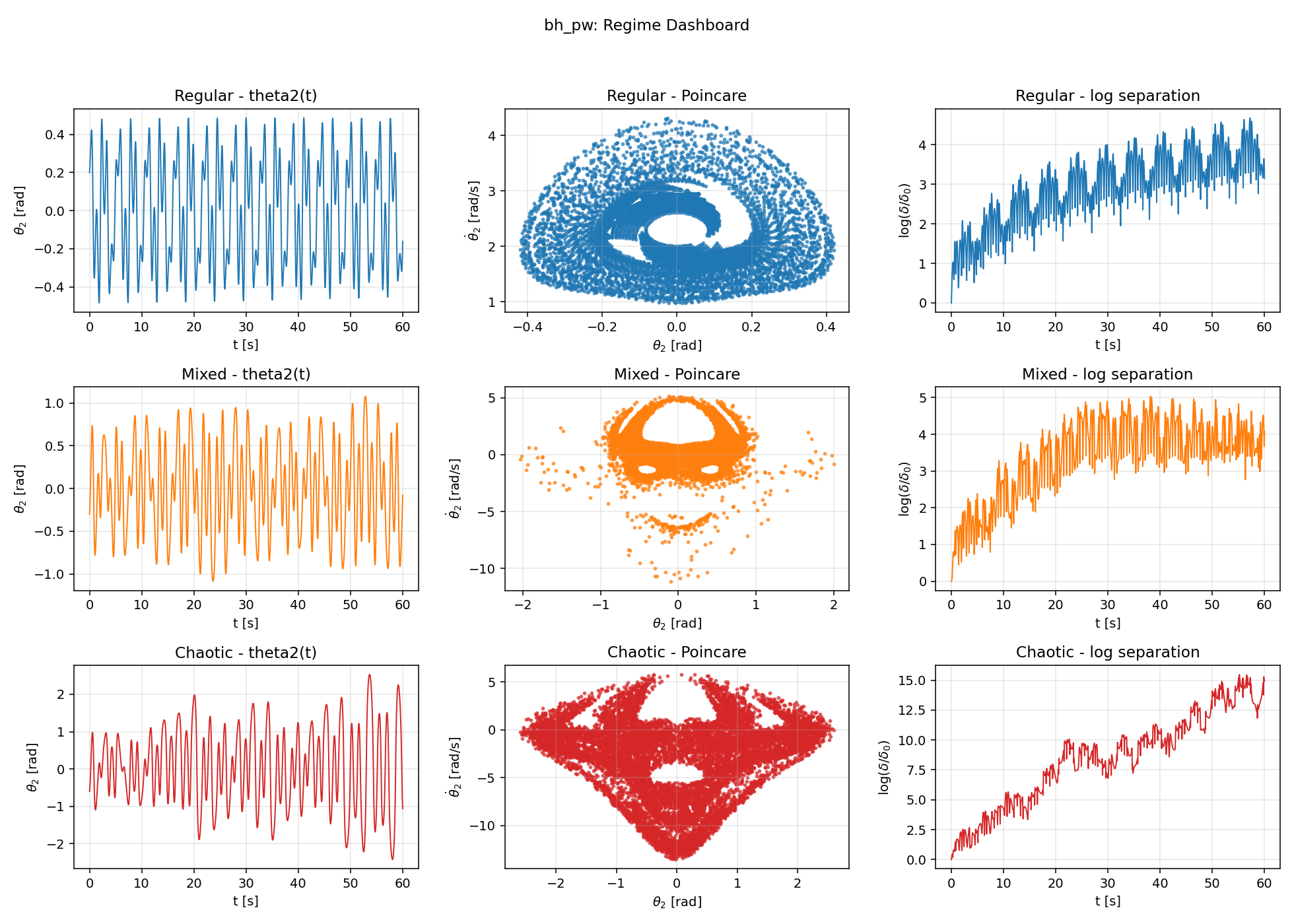
Three representative initial-condition regimes were used throughout: regular $[0.9,\ 0.2,\ 0.0,\ 0.3]$ , mixed $[1.1,\ {-0.3},\ 0.0,\ 0.8]$ , and chaotic $[1.3,\ {-0.6},\ 0.0,\ 1.2]$ (formatted as $[\theta_1,\ \theta_2,\ \dot{\theta}_1,\ \dot{\theta}_2]$ ). These three states were selected by inspection of a preliminary $\dot{\theta}_2(0)$ scan under uniform_g and verified by their FTLE values (Table 2): the regular IC sits in a region of closed Poincaré curves with low $\lambda$ , the chaotic IC sits in the scattered, area-filling region with the highest $\lambda$ , and the mixed IC straddles them.

A scan over the initial angular velocity $\dot{\theta}_2(0)$ was used to produce a Poincaré-response (bifurcation-style) diagram for each model. $\dot{\theta}_2(0)$ was swept from 0.0 to 1.8 rad/s in 80 steps. For each scan value, 100 section points were recorded after discarding the first 60% of crossings as transient. The 60% threshold was checked by recomputing the bifurcation diagrams at thresholds of 0.3, 0.4, 0.5, 0.7, and 0.8: the standard deviation of $\theta_2$ across the scan varied by $\leq 1$ % (uniform_g) and $\leq 3$ % (linear_y), confirming the bifurcation structure is insensitive to choice.

Reproducibility details

Mechanical parameters: $m_1 = m_2 = 1.0$ kg; $L_1 = L_2 = 1.0$ m; $g_0 = 9.81\ \mathrm{m\,s^{-2}}$ . $\theta_1$ measured from downward vertical and $\theta_2$ measured from the first link; $y$ is positive upward. Pivot at the origin for uniform_g and linear_y; at $(0,\ R_{\mathrm{pivot}})$ for bh_pw. Bob positions: for uniform_g/linear_y, $y_1 = -L_1 \cos\theta_1$ and $y_2 = y_1 - L_2\cos(\theta_1 + \theta_2)$ ; for bh_pw, $\mathbf{r}1 = (L_1\sin\theta_1,\ R{\mathrm{pivot}} - L_1\cos\theta_1)$ and $\mathbf{r}_2 = \mathbf{r}_1 + (L_2\sin(\theta_1+\theta_2),\ -L_2\cos(\theta_1+\theta_2))$ . The equations of motion are $M(q)\ddot{q} + C(q,\dot{q}) + \nabla U(q) = 0$ with

M_{11} = (m_1+m_2)L_1^2 + m_2 L_2^2 + 2m_2 L_1 L_2 \cos\theta_2,

M_{12} = M_{21} = m_2 L_2^2 + m_2 L_1 L_2 \cos\theta_2,

M_{22} = m_2 L_2^2,

and $C(q,\dot{q}) = \bigl(-m_2 L_1 L_2 \sin\theta_2 (2\dot{\theta}_1\dot{\theta}_2 + \dot{\theta}_2^2),\ m_2 L_1 L_2 \sin\theta_2\,\dot{\theta}_1^2\bigr)$ . The gravity model (Methods § Gravity field models”) determines the value of $U(q)$ . Poincaré crossings are observed at $\sin\theta_1 = 0$ and $\cos\theta_1 > 0$ , and $\dot{\theta}_1 > 0$ . The 12-IC Gaussian cloud (Results §FTLE convergence”) is generated with the numpy default_rng, with seed = 42. All scripts, parameter files and raw output tables can be found in the gravity-double-pendulum GitHub repository (https://github.com/virajsaraogi613-code/gravity-double-pendulum).

Additional one-factor parameter sweeps were performed for the chaotic regime only: $L_2/L_1 \in [0.6,\ 0.8,\ 1.0,\ 1.2,\ 1.4,\ 1.6]$ , $m_2/m_1 \in [0.5,\ 0.75,\ 1.0,\ 1.25,\ 1.5,\ 2.0]$ , and for linear_y, $\mathrm{d}g/\mathrm{d}y \in [-2.0,\ {-1.0},\ {-0.5},\ 0.0,\ 0.5,\ 1.0,\ 2.0]\ \mathrm{m\,s^{-2}\,m^{-1}}$ . Both $\lambda$ and $\lambda^*$ were calculated for each sweep point.

Results

Sampling quality and numerical stability

Across all models, ensemble Poincaré projections were densely sampled and energy drift remained extremely small, indicating stable integration. For uniform_g, drift ranged from $-5.95\times10^{-9}$ % to $4.91\times10^{-11}$ % with 13,112–17,998 section points (Table 1). For linear_y, drift ranged from $-3.96\times10^{-9}$ % to $-1.93\times10^{-12}$ % with 11,737–16,468 section points (Table 1). For bh_pw, drift ranged from $-1.49\times10^{-12}$ % to $2.21\times10^{-12}$ % with 4,651–12,978 section points depending on body and regime (Table 1).

Model	Energy drift range (%)	Section points (range across regimes)
uniform_g	−5.95×10⁻⁹ to 4.91×10⁻¹¹	13,112 to 17,998
linear_y	−3.96×10⁻⁹ to −1.93×10⁻¹²	11,737 to 16,468
bh_pw (Configs I, II, III)	−1.49×10⁻¹² to 2.21×10⁻¹²	4,651 to 12,978

Table 1 | Sampling quality. Energy drift bounds and Poincaré section-point counts across the three gravity models, aggregated across the regular, mixed, and chaotic regimes.

Uniform gravity baseline

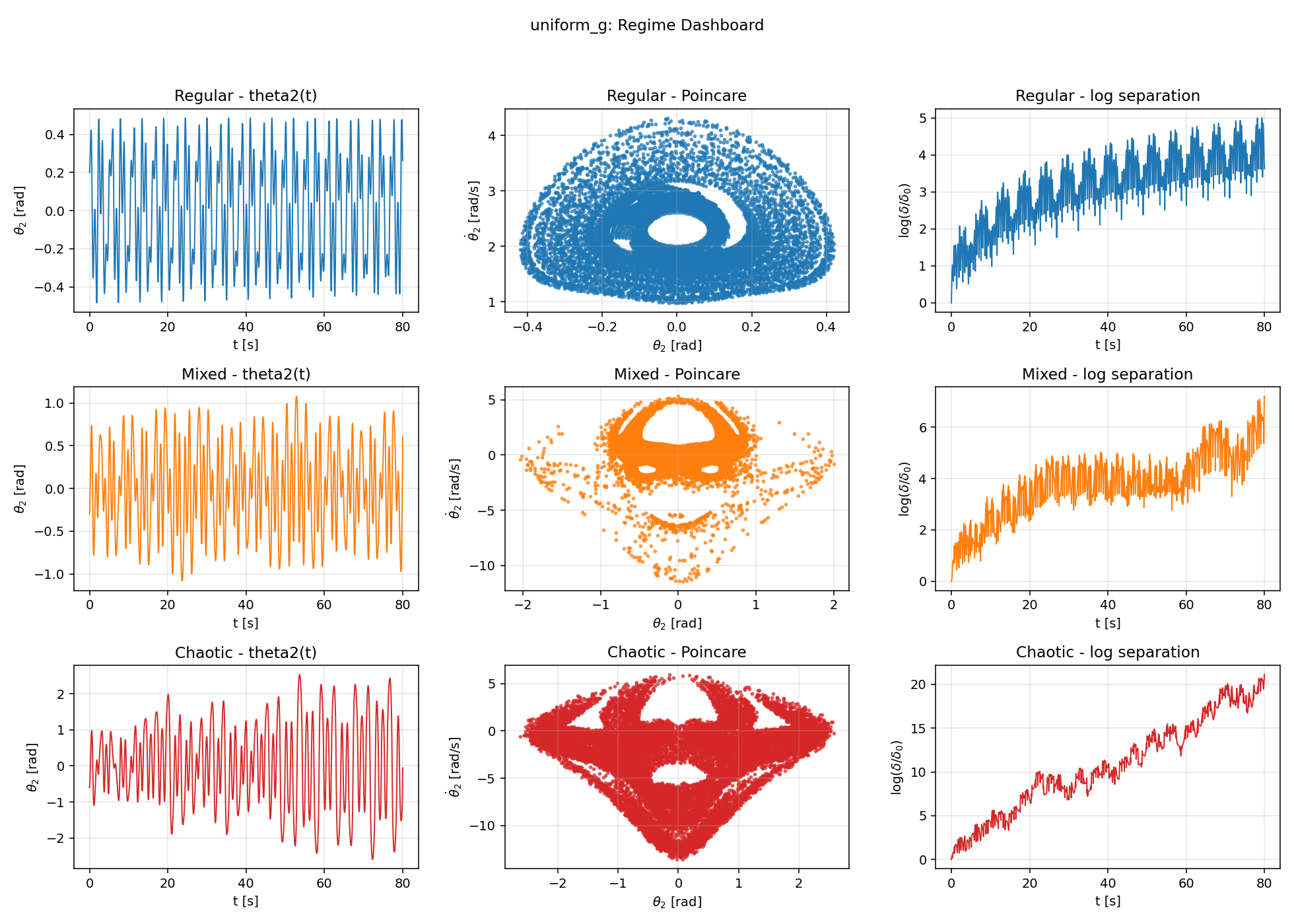
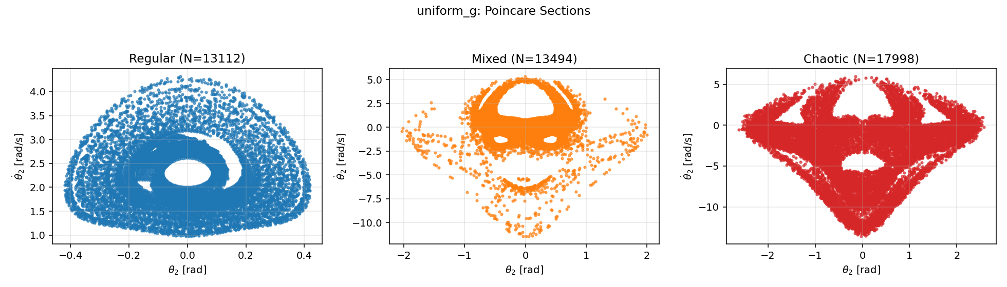
Under uniform_g, the three regimes exhibited increasing sensitivity to initial conditions and increasing phase-space filling in the ensemble Poincaré projection (Figures 1 and 2). The FTLE increased from $\lambda = 0.052$ 1/s ( $\lambda^* = 0.0168$ ) in the regular case to $\lambda = 0.068$ 1/s ( $\lambda^* = 0.0217$ ) in the mixed case, and to $\lambda = 0.248$ 1/s ( $\lambda^* = 0.0793$ ) in the chaotic case (Table 2).

Figure 1 | Phase-space trajectories for the uniform gravity model across the three initial-condition regimes. Increasing trajectory complexity from regular to chaotic is evident in the shape and spread of the curves.

Figure 2 | Ensemble Poincaré projections for the uniform gravity model. Closed curves indicate quasi-periodic motion (regular regime); scattered points indicate chaos (chaotic regime).

Regime	λ (1/s)	λ*
regular	0.052	0.0168
mixed	0.068	0.0217
chaotic	0.248	0.0793

Table 2 | λ and dimensionless λ* per regime under uniform gravity (uniform_g).

Linear vertical gravity gradient

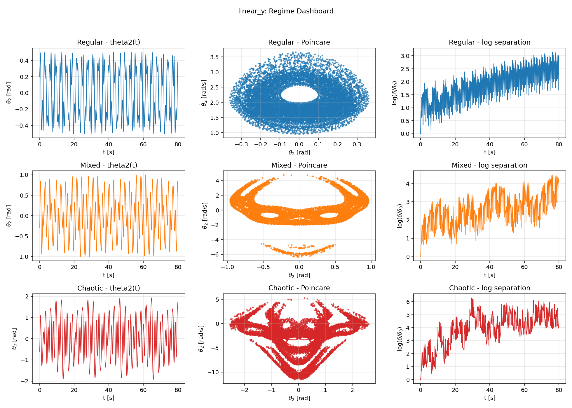
Introducing a linear_y gravity gradient altered the qualitative structure of the ensemble Poincaré projections and reduced the FTLE for the chaotic initial condition relative to the uniform baseline (Figures 3 and 4). In linear_y, the regular and mixed regimes had $\lambda$ = 0.030 1/s ( $\lambda^$ = 0.0095) and $\lambda$ = 0.064 1/s ( $\lambda^$ = 0.0206), respectively. The chaotic regime decreased to $\lambda$ = 0.067 1/s ( $\lambda^$ = 0.0213), compared to $\lambda^$ = 0.0793 under uniform_g (Table 4).

Figure 3 | Phase-space trajectories for the linear gravity gradient model. Compared to Figure 1, the chaotic trajectory shows reduced spread, consistent with lower phase-space stretching under the gradient field.

Regime	λ (1/s)	λ*
regular	0.030	0.0095
mixed	0.064	0.0206
chaotic	0.067	0.0213

Table 3 | λ and λ* per regime under the linear vertical gradient (linear_y).

Figure 4 | Side-by-side ensemble Poincaré projections for the chaotic initial condition across all gravity models. The linear gradient and Configuration I (ε ≈ 11.27) pseudo-Newtonian cases show markedly more structured, less area-filling sections.

Model / Configuration	Regular λ*	Mixed λ*	Chaotic λ*
uniform_g	0.0168	0.0217	0.0793
linear_y	0.0095	0.0206	0.0213
bh_pw Config I	0.0027	0.0009	0.0010
bh_pw Config II	0.0311	0.0248	0.0775
bh_pw Config III	0.0311	0.0244	0.0802

Table 4 | Cross-model comparison of dimensionless λ* across the three initial-condition regimes.

Pseudo-Newtonian (Paczynski-Wiita) gravity

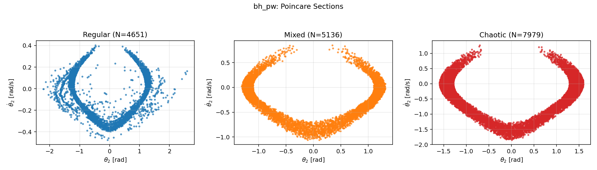
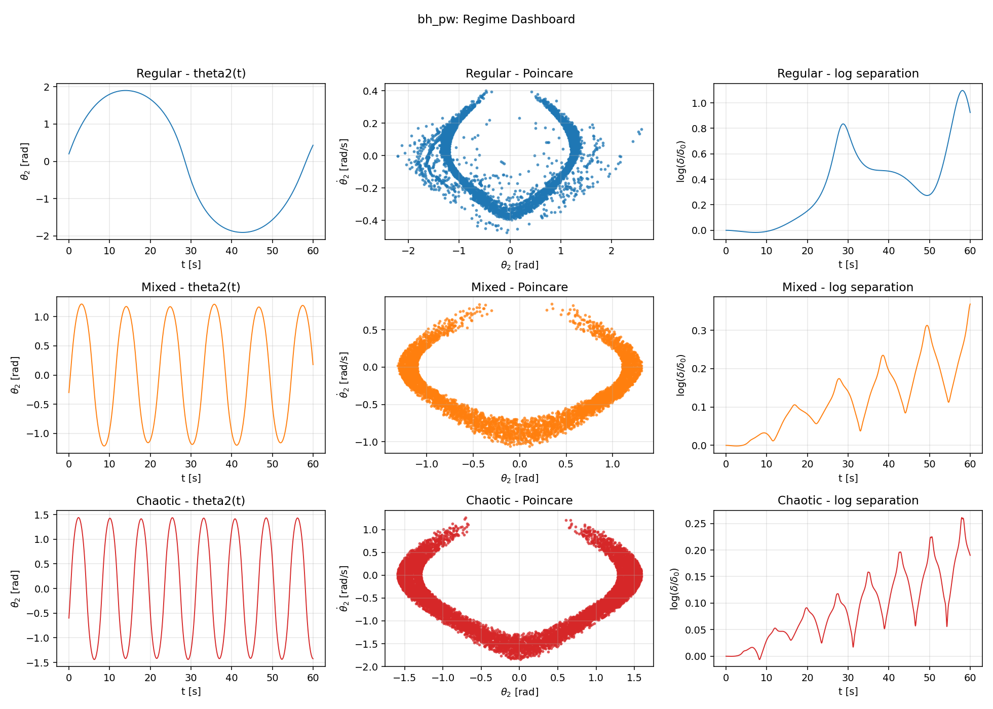
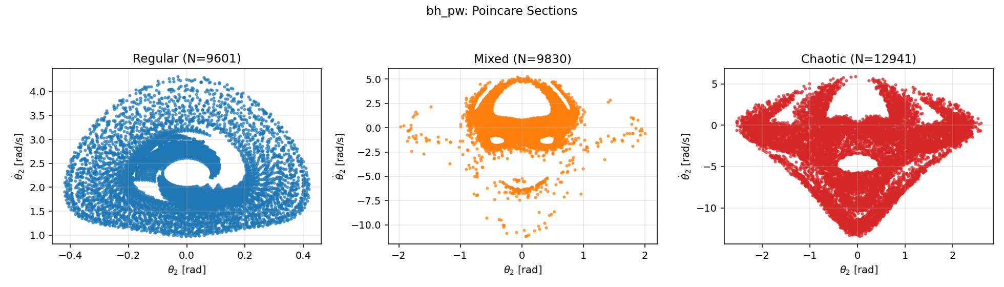
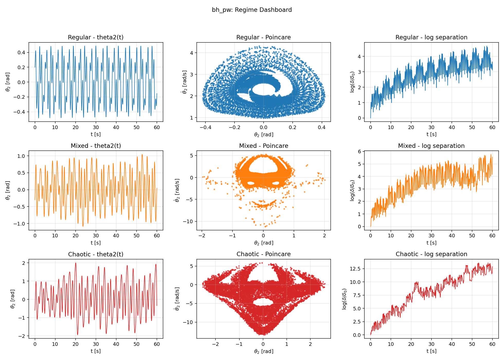
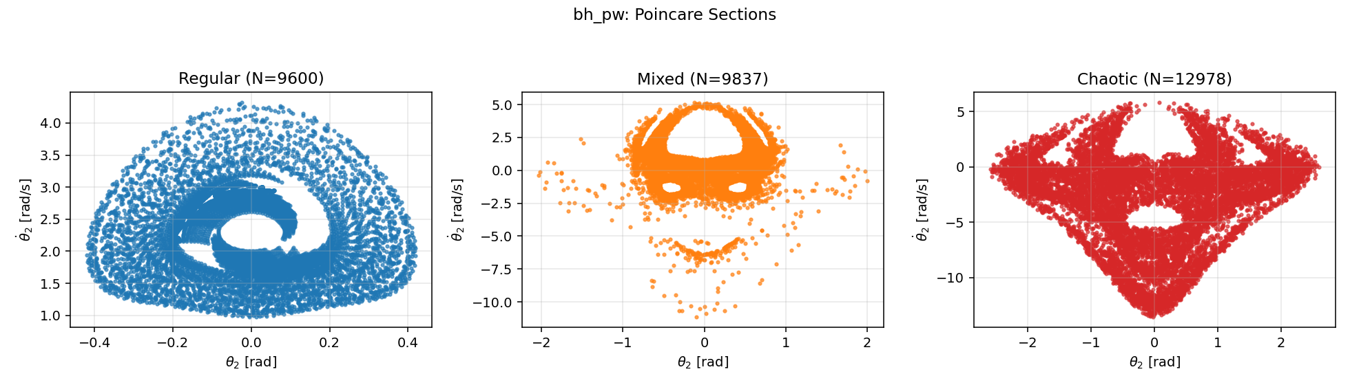
The bh_pw model was evaluated for Configurations I, II, and III, each calibrated so that the local acceleration magnitude at the pivot matched $g_{\mathrm{ref}} = 9.81\ \mathrm{m\,s^{-2}}$ . The resulting ensemble Poincaré projections and FTLEs differed strongly between the Configuration I ( $\varepsilon \approx 11.27$ ) case and the Configurations II and III cases (Figures 4, 5a, 6a, 7a).

For Configuration I ( $\varepsilon \approx 11.27$ ), FTLEs were $\lambda = 0.0085$ , $0.0027$ , $0.0030$ 1/s for regular, mixed, and chaotic regimes, respectively ( $\lambda^* = 0.0027$ , $0.0009$ , $0.0010$ ).

For Configuration II ( $\varepsilon \approx 3.39 \times 10^{-5}$ ), FTLEs were $\lambda = 0.0975$ , $0.0776$ , $0.2426$ 1/s for regular, mixed, and chaotic regimes, respectively ( $\lambda^* = 0.0311$ , $0.0248$ , $0.0775$ ).

For Configuration III ( $\varepsilon \approx 7.88 \times 10^{-12}$ ), FTLEs were $\lambda = 0.0974$ , $0.0765$ , $0.2513$ 1/s for regular, mixed, and chaotic regimes, respectively ( $\lambda^* = 0.0311$ , $0.0244$ , $0.0802$ ).

A $4\times4$ scan over $\varepsilon \in {10^{-3},\ 10^{-2},\ 10^{-1},\ 3\times10^{-1}}$ and $k \in {3,\ 10,\ 30,\ 100}$ for the chaotic IC (Table 6) gave $\lambda^$ in $[0.064,\ 0.391]$ across 15 valid cells; the ( $\varepsilon = 3\times10^{-1}$ , $k = 3$ ) cell hits the toy-potential safety boundary. A mass-invariance check at fixed ( $\varepsilon = 0.01$ , $k = 10$ ) varied $g_{\mathrm{target}}$ by four orders of magnitude with integration horizon and IC velocities scaled to preserve the dimensionless state; $\lambda^$ varied by 7.6% (rel. std., Table 7). Both confirm the dimensionless framing.

ε \ k	k = 3	k = 10	k = 30	k = 100
10⁻³	0.0653	0.0999	0.1185	0.0821
10⁻²	0.0641	0.0893	0.1100	0.0936
10⁻¹	0.1174	0.0947	0.0978	0.1148
3 × 10⁻¹	—	0.3661	0.3910	0.3143

Table 5 | Dimensionless λ* across the 4×4 (ε, k) scan under the pseudo-Newtonian potential, chaotic IC. The (ε ≈ 0.3, k = 3) cell is geometrically inaccessible (toy-potential safety boundary).

g_target (m/s²)	λ (1/s)	λ*
0.1	0.0253	0.0800
1.0	0.0828	0.0828
9.81	0.2798	0.0893
98.1	0.9638	0.0973

Table 6 | Mass-invariance check at fixed (ε = 0.01, k = 10). Integration horizon and IC velocities scaled so that the dimensionless state is preserved across g_target.

Figure 5a | Poincaré sections for the Configuration I (ε ≈ 11.27) pseudo-Newtonian model. All three regimes exhibit thin, curve-like structures, consistent with quasi-periodic motion and very low FTLE values (λ* ∼ 10⁻³).

Figure 5b | Phase-space trajectory dashboard for the Configuration I (ε ≈ 11.27) pseudo-Newtonian model. All three regimes show smooth, low-amplitude oscillations consistent with quasi-periodic motion.

Figure 6a | Poincaré sections for the Configuration II (ε ≈ 3.39 × 10⁻⁵) pseudo-Newtonian model. Phase-space structure closely resembles the uniform gravity baseline, reflecting the near-uniform field experienced at R_pivot ≫ L.

Figure 6b | Phase-space trajectory dashboard for the Configuration II (ε ≈ 3.39 × 10⁻⁵) pseudo-Newtonian model. The chaotic regime (red) shows the irregular, high-amplitude swings characteristic of strong chaos.

Figure 7a | Ensemble Poincaré projections for the Configuration III pseudo-Newtonian model. Results are nearly identical to the Configuration II (ε ≈ 3.39 × 10⁻⁵) case, confirming that dynamics are governed by the L/R_pivot ratio rather than absolute mass when g_ref is matched.

Figure 7b | Phase-space trajectory dashboard for the Configuration III pseudo-Newtonian model. Results are nearly identical to the Configuration II (ε ≈ 3.39 × 10⁻⁵) case, confirming that dynamics scale with L/R_pivot.

Configuration (ε)	Regime	λ (1/s)	λ*
I (ε ≈ 11.27)	regular	0.0085	0.0027
I	mixed	0.0027	0.0009
I	chaotic	0.0030	0.0010
II (ε ≈ 3.39×10⁻⁵)	regular	0.0975	0.0311
II	mixed	0.0776	0.0248
II	chaotic	0.2426	0.0775
III (ε ≈ 7.88×10⁻¹²)	regular	0.0974	0.0311
III	mixed	0.0765	0.0244
III	chaotic	0.2513	0.0802

Table 7 | λ and λ* per regime for the three pseudo-Newtonian configurations.

Parameter sweep results (chaotic regime)

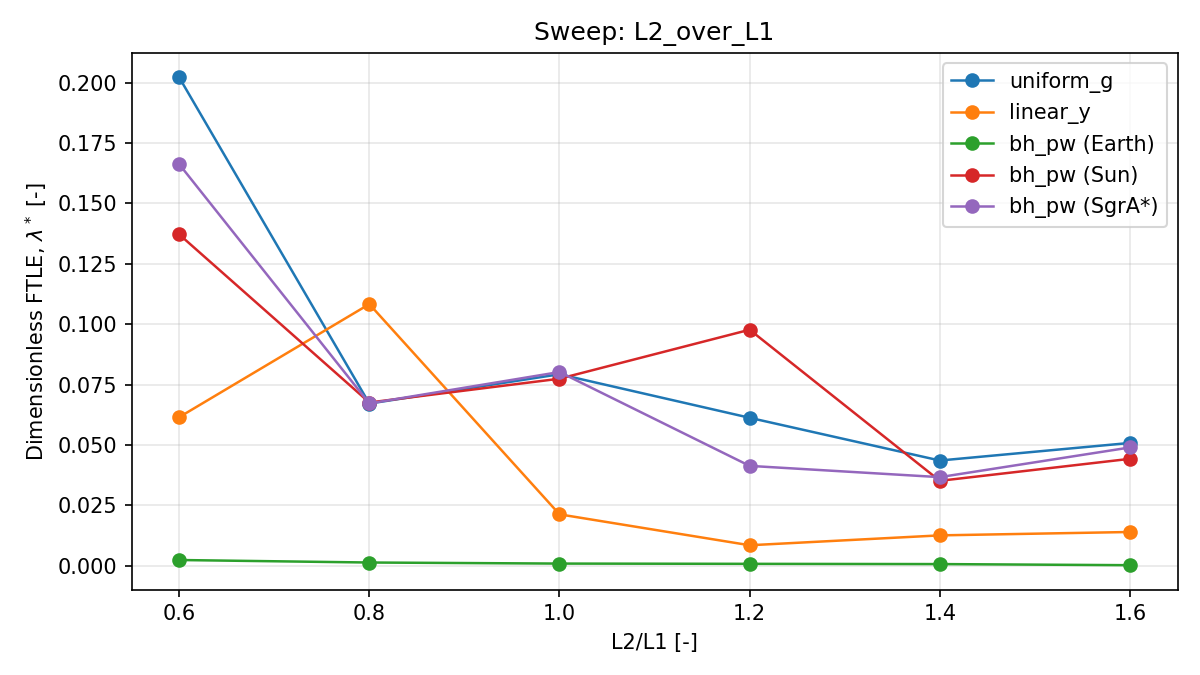
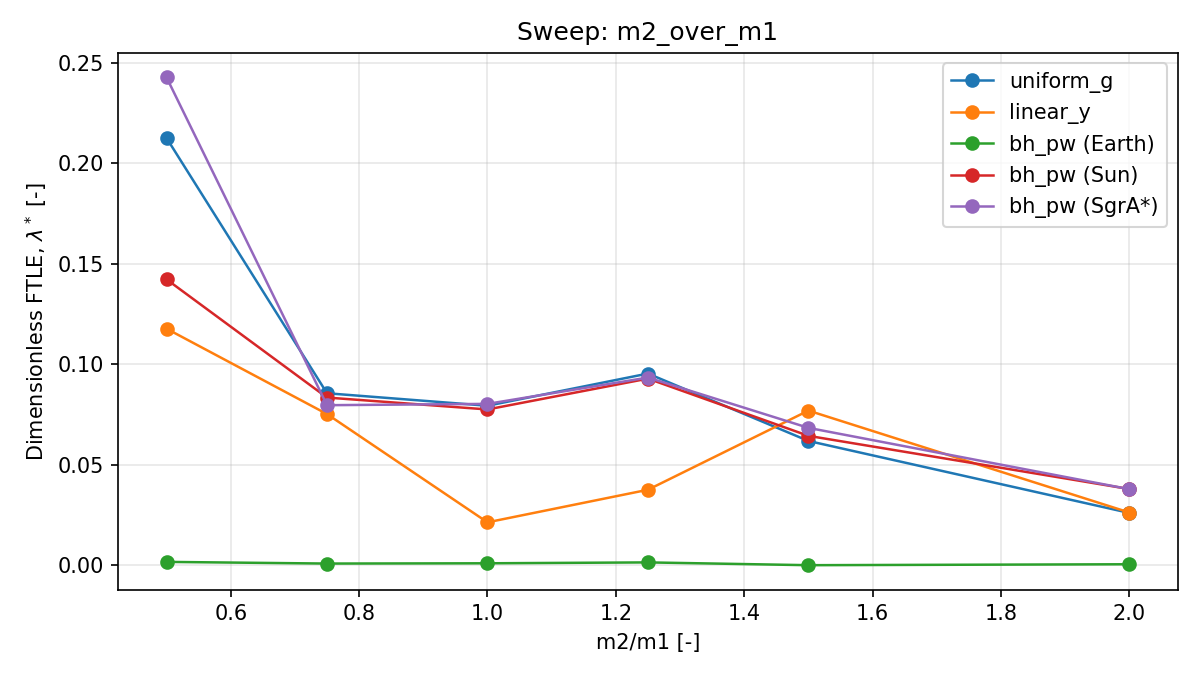
One-factor sweeps quantified how geometry, mass distribution, and gravity gradient modulate chaos strength. In uniform_g, the strongest chaos over the tested grid occurred at $L_2/L_1 = 0.6$ ( $\lambda^* = 0.202$ ) and $m_2/m_1 = 0.5$ ( $\lambda^* = 0.212$ ), with decreasing $\lambda^$ as these ratios increased (Figures 8 and 9). In linear_y, the peak shifted to $L_2/L_1 = 0.8$ ( $\lambda^ = 0.108$ ) and $m_2/m_1 = 0.5$ ( $\lambda^* = 0.118$ ), while a pronounced minimum occurred at $L_2/L_1 = 1.2$ ( $\lambda^* = 0.00854$ ).

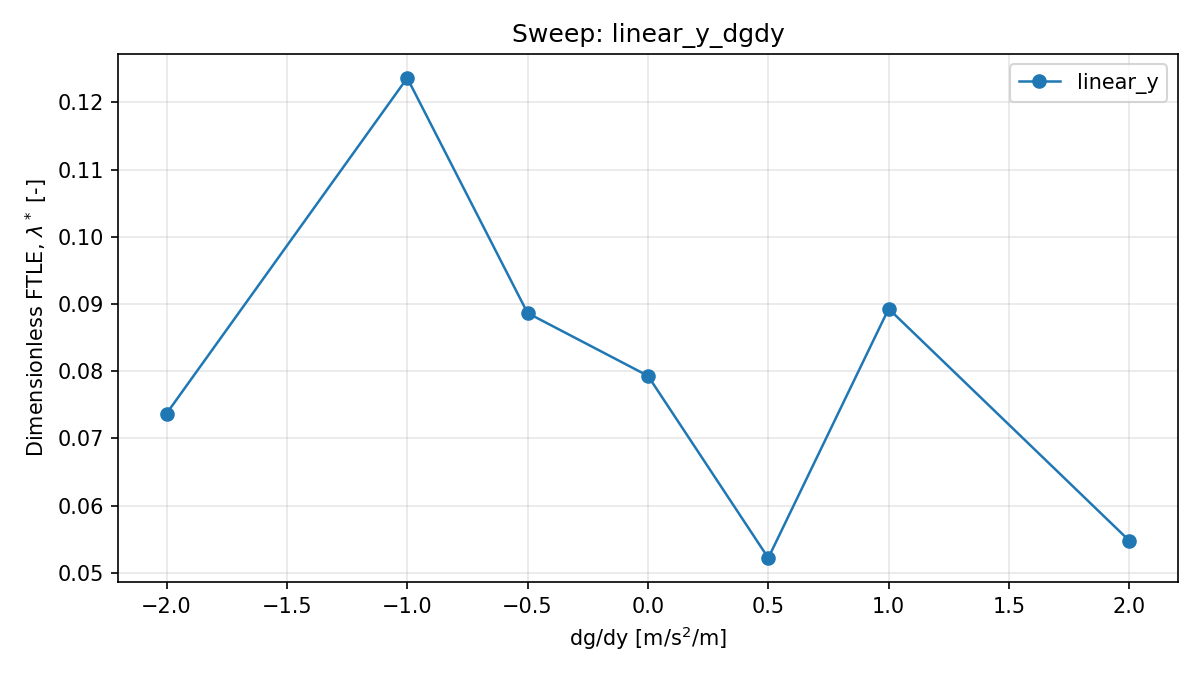
The gravity-gradient sweep in linear_y was non-monotonic and sign-dependent (Figure 10). Over $\mathrm{d}g/\mathrm{d}y \in [-2,\ 2]\ \mathrm{m\,s^{-2}\,m^{-1}}$ , the largest $\lambda^$ occurred at $\mathrm{d}g/\mathrm{d}y = -1.0$ ( $\lambda^ = 0.124$ ), while the smallest tested value occurred at $\mathrm{d}g/\mathrm{d}y = +0.5$ ( $\lambda^* = 0.0522$ ).

For bh_pw, Configurations II and III ( $\varepsilon \ll 1$ ) followed trends similar to uniform_g, with peak $\lambda^$ again at $L_2/L_1 = 0.6$ and $m_2/m_1 = 0.5$ . In contrast, Configuration I ( $\varepsilon \approx 11.27$ ) yielded $\lambda^$ near $10^{-3}$ across the sweep range, consistent with substantially more regular motion under that parameterization.

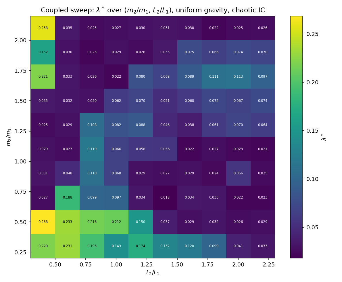
A $10\times10$ coupled sweep over $(m_2/m_1,\ L_2/L_1)$ under uniform_g, chaotic IC (Figure 11) gave $\lambda^*$ in $[0.018,\ 0.268]$ , peaking at $(0.50,\ 0.40)$ and minimising at $(0.70,\ 1.40)$ . The 1D slices at $m_2/m_1 = 1$ and $L_2/L_1 = 1$ recover the earlier single-parameter trends; the off-diagonal structure indicates the two ratios do not act fully independently at small $m_2/m_1$ .

Figure 8 | FTLE (λ*) as a function of link-length ratio L2/L1 for all gravity models in the chaotic regime. Peak chaos occurs at L2/L1 = 0.6 under uniform gravity and the Configurations II and III pseudo-Newtonian model; a pronounced minimum appears near L2/L1 = 1.2 for the linear gradient model.

*Figure 9 | FTLE (λ*) as a function of mass ratio m2/m1 for all gravity models in the chaotic regime. Chaos strength decreases as m2/m1 increases across all models, with peak values at m2/m1 = 0.5.*

Figure 10 | FTLE (λ*) as a function of gravity gradient strength dg/dy for the linear gradient model. The response is non-monotonic: the largest λ* occurs at dg/dy = −1.0 m/s²/m, while a minimum appears near dg/dy = +0.5 m/s²/m.

Figure 11 | λ* over the coupled (m₂/m₁, L₂/L₁) grid under uniform_g, chaotic IC. Numeric values shown in each cell. Peak λ* = 0.268 at (m₂/m₁ = 0.50, L₂/L₁ = 0.40).

FTLE convergence and uncertainty

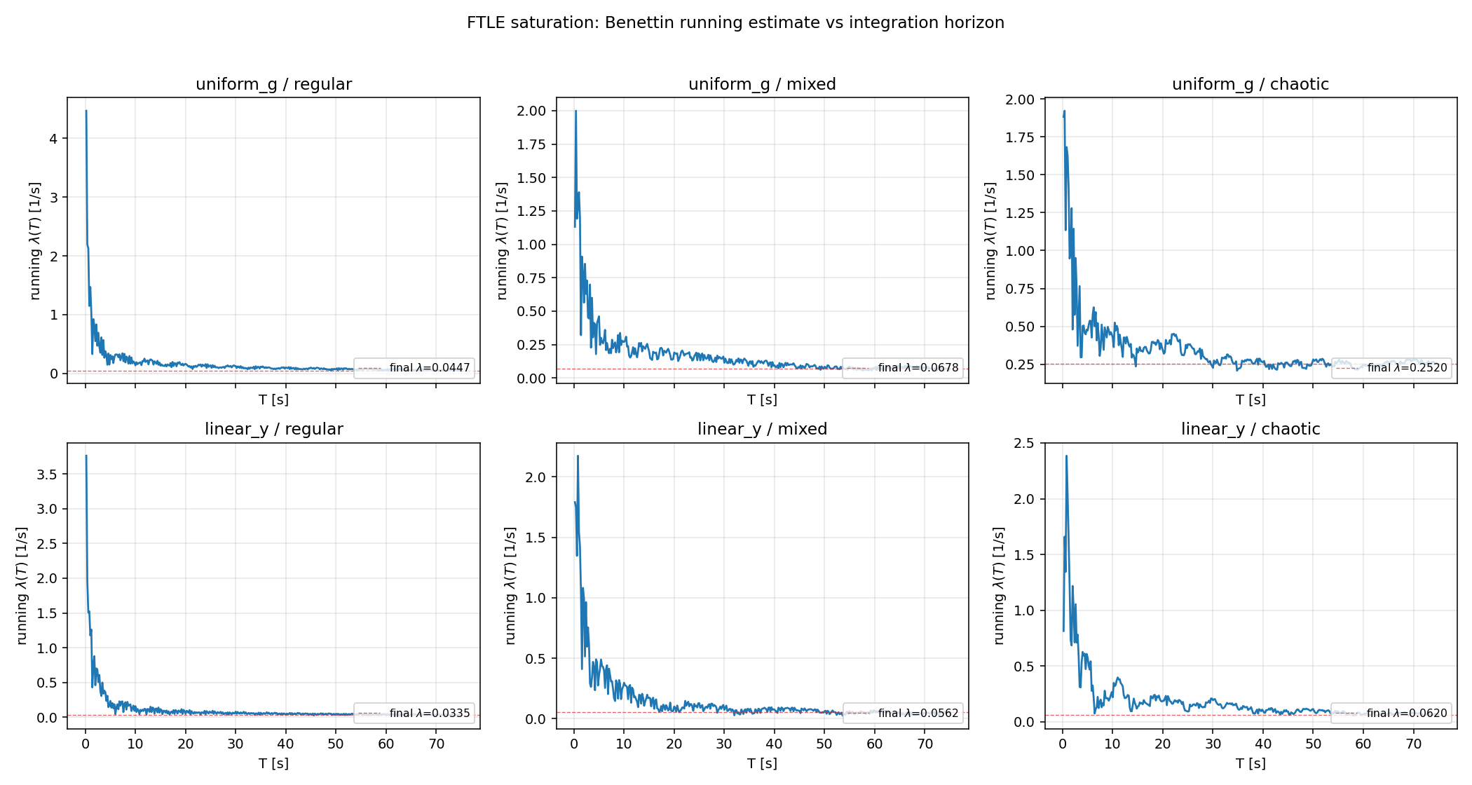
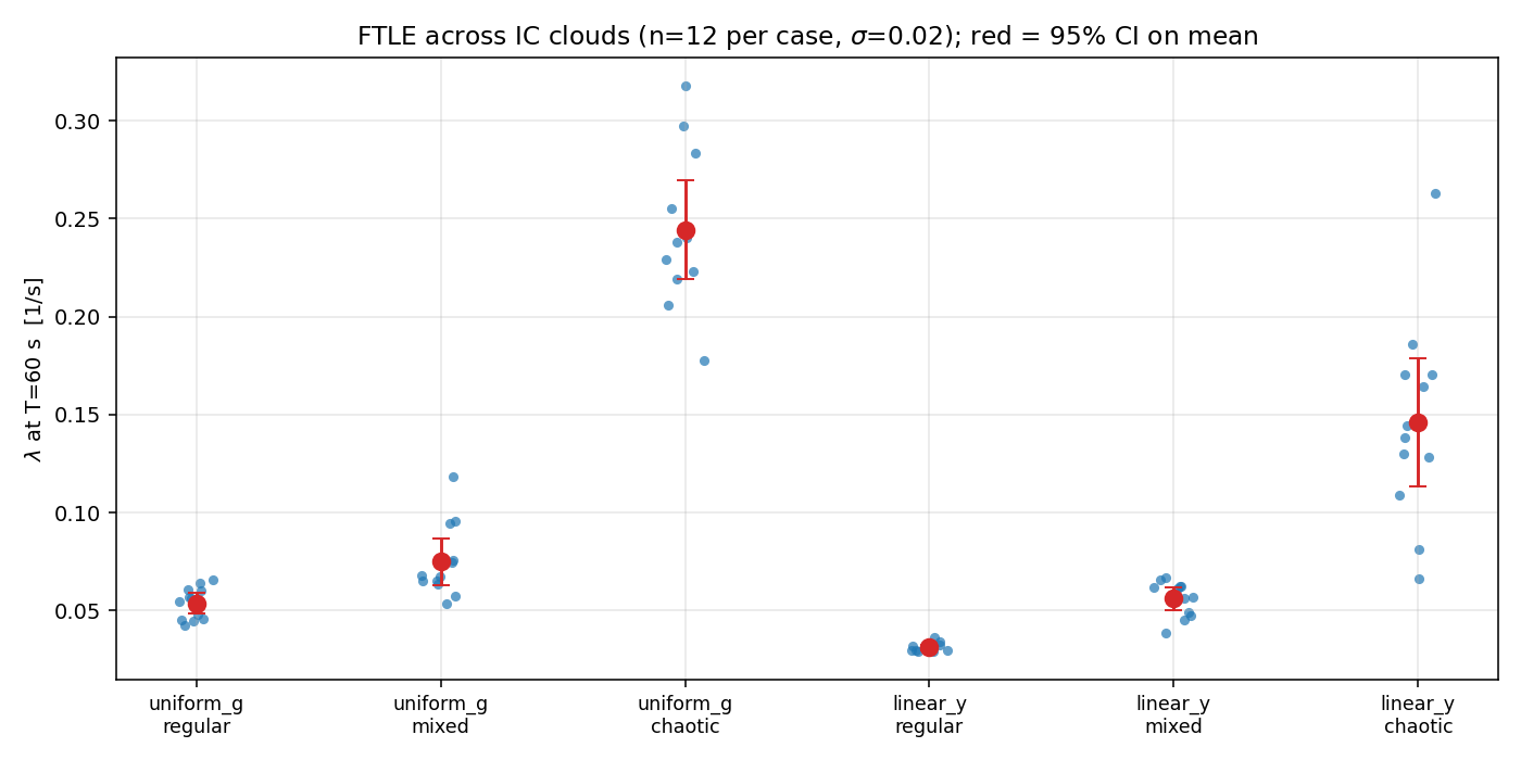
We ran two convergence diagnostics on uniform_g and linear_y. The $\lambda(T)$ curves up to $T = 75$ s saturated well before $T_{\max}$ for all three regimes in both models (Figure 12). A Gaussian cloud of 12 nearby ICs ( $\sigma = 0.02$ , seed $= 42$ ) at $T = 60$ s gave mean $\lambda = 0.244$ for uniform_g chaotic (95% CI $[0.219,\ 0.269]$ ) and $0.146$ for linear_y chaotic (95% CI $[0.113,\ 0.179]$ ); the much wider linear_y cloud ( ${\approx}3\times$ range in $\lambda$ ) indicates the canonical linear_y chaotic IC sits near a basin boundary (Figure 13).

Figure 12 | Running λ(T) estimates for the three regimes under uniform_g (top) and linear_y (bottom), T up to 75 s. All curves level off well before T_max, with the final value marked by a dashed line.

Figure 13 | λ values from 12-IC Gaussian clouds (σ = 0.02) around each canonical IC at T = 60 s. Red bars show 95% CIs on the mean. The linear_y chaotic case (rightmost) shows the widest cloud, consistent with the canonical IC sitting near a basin boundary.

Discussion

Different interpretations of chaos in gravity models

The gravity model was applied to the same mechanical parameters and initial conditions, and altered both the local restoring forces and the potential-energy landscape geometry, which resulted in a change of the phase-structures observed in ensemble Poincaré maps. The linear_y model proved to be the case with the most evident regime shift: the initial condition chaotic under uniform_g had significantly smaller $\lambda$ and $\lambda^*$ , and its ensemble Poincaré plot was more banded with a lower density of points filling the space. This means that for some trajectories, phase space stretching is reduced by the addition of a vertical gravity gradient and for other regimes the change in phase space stretching is not that large. If the gradient is positive, then the restoring torque is enhanced for large amplitude swings, and chaotic swings are damped, because gravity is greater when the bob swings above the pivot. The opposite is done by a negative gradient. This is consistent with the bifurcation sweep, where the value of the chaos parameter $\mathrm{d}g/\mathrm{d}y$ is maximum at negative $\mathrm{d}g/\mathrm{d}y$ and minimum near $\mathrm{d}g/\mathrm{d}y \approx +0.5\ \mathrm{m\,s^{-2}\,m^{-1}}$ , and is closely related to the general set of asymmetrical conditions being a control parameter for the appearance of chaos in coupled oscillators²⁶.

These effects are not monotonic and the parameter sweeps confirm this. The influence of chaos strength on the linear_y was very strong in terms of the link-length ratio, as well as sign and magnitude of $\mathrm{d}g/\mathrm{d}y$ . It is seen that the gradient has an interaction with the effective frequencies and coupling terms in the pendulum, leading to islands of stability and narrow windows of increased chaos, rather than a universal trend of `more gradient $\to$ more chaos’.

Why the present setup requires the use of the variable ε for bh_pw?

For all configurations ( $k = R_{\mathrm{pivot}}/r_s = 10$ constant) the same link lengths ( $L_1 = L_2 = 1$ m) were used and the pivot was located at $R_{\mathrm{pivot}} = 10\,r_s$ . The three configurations thus differ only in the dimensionless ratio $\varepsilon = L_1/R_{\mathrm{pivot}} \approx 11.27$ , $3.39 \times 10^{-5}$ and $7.88 \times 10^{-12}$ for Configurations I, II, and III, respectively. In Configuration I, with $\varepsilon > 1$ , the lengths of the links (1 m each) are larger than the distance $R_{\mathrm{pivot}} \approx 0.0887$ m and the bob trajectories pass through a very nonuniform and direction-changing central field. The results of the trajectories tested were consistent with quasi-periodic motion, with small $\lambda^*$ ( ${\sim}10^{-3}$ ) and with thin curves in Poincaré sections.

In Configurations II and III, $r_s$ is on the kilometre to astronomical scale, in which case $R_{\mathrm{pivot}}$ is quite large compared to 1 m links. In this limit, the field felt by the pendulum is almost constant during its motion and the ensemble Poincaré projections and $\lambda^*$ values are very close to the uniform_g base line. Hence the difference in the body-to-body characteristics of the experiments conducted here is mainly due to the scaling ratio $L/R_{\mathrm{pivot}}$ and not to any intrinsic mass dependence at a fixed value of $g_{\mathrm{ref}}$ at the pivot.

Implications

Based on the obtained results, it is possible to draw a practical conclusion: the nonuniformity of gravity can be used as a control parameter in chaotic studies of coupled mechanical systems. Even a very modest linear gradient can alter which geometries maximize chaos and can decrease $\lambda^*$ , and can even cause the phase space structure of trajectories that are chaotic in uniform gravity to look squashed. This bridges a textbook chaotic system (double pendulum) with gravity-gradient environments important to central-field dynamics, but retains the ease of analysis by standard phase-space tools.

Limitations

There are a few physical modelling caveats. The model of the bh_pw is a pseudo-Newtonian model that does not describe full general relativity; it describes a radial divergence that is very strong, but it ignores any effects related to curvature of spacetime on constraints and time dilation. The model linear_y is a theoretical vertical gradient and is not meant to be a quantitatively accurate model of Earth or solar gravity over meters; rather it is used to test for qualitative sensitivity to gravity inhomogeneity. Idealization of the mechanical system is assumed (massless rods, no damping, no driving) in real double pendula, friction and flexing can change the long time behavior and introduce attractors.

There are caveats to the chaos diagnostics, too. FTLE values are finite time estimates and are window and renormalization schedule dependent, but they represent values of predictability over the selected time window and not an asymptotic value of the Lyapunov spectrum. Bifurcation-style plots are Poincaré-response diagrams versus initial-condition scans; for conservative systems, these should not be used as attractor bifurcation in a strict sense as used for dissipative systems. The reduction of FTLE is a necessary but not sufficient condition for the full sense of chaos suppression; additional analyses like changes in phase-space volume, invariant-measure properties, or full Lyapunov-spectrum verification are needed to prove suppression as indicated in the Future work section.

Future work

There are several extensions to the above, naturally. First, a central field Newtonian model with realistic radii for Earth and Sun ( $\varphi = -GM/r$ ) could be used, in addition to “exaggerated” cases with fixed $\varepsilon = L/R$ , which could emphasize the effects of scaling. Second, the current dimensionless pseudo-Newtonian study can be expanded by increasing the density of the scans of $k = R_{\mathrm{pivot}}/r_s$ and link-length ratios to better characterize the transition from chaotic to quasi-periodic behavior. Third, other chaos diagnostics, such as recurrence plots, the 0–1 test, or a set of multiple Lyapunov exponents, could provide cross-validation of the trends in FTLEs reported herein. Fourth, quantitative KAM diagnostics (e.g., resonance overlap, detection of invariant tori) would aid in the connection of the gravity-model effects with KAM theory.

Conclusion

Of the three gravity models, the linear gradient decreased the chaotic-regime $\lambda^*$ from 0.079 to 0.021, in the bifurcation sweep, the chaotic behavior was most prominent at negative $\mathrm{d}g/\mathrm{d}y$ , and was at its lowest around $+0.5\ \mathrm{m\,s^{-2}\,m^{-1}}$ . The pseudo-Newtonian dynamics are set by $\varepsilon = L_1/R_{\mathrm{pivot}}$ and $k = R_{\mathrm{pivot}}/r_s$ rather than by mass, as is confirmed by the $(\varepsilon, k)$ scan and a mass-invariance check. The single-parameter trends were recovered by a coupled sweep $(m_2/m_1 \times L_2/L_1)$ under uniform gravity with mild interaction at small $m_2/m_1$ . This means that gravity-field geometry can be considered as a chaos control parameter for coupled mechanical systems.

References

T. Shinbrot, C. Grebogi, J. Wisdom, J. A. Yorke. Chaos in a double pendulum. American Journal of Physics. Vol. 60, pg. 491–499, 1992, https://doi.org/10.1119/1.16860. [↩]
S. H. Strogatz. Nonlinear dynamics and chaos: With applications to physics, biology, chemistry, and engineering. Westview Press, 2014. [↩] [↩]
E. N. Lorenz. Deterministic nonperiodic flow. Journal of the Atmospheric Sciences. Vol. 20, pg. 130–141, 1963, https://doi.org/10.1175/1520-0469(1963)020%3C0130:DNF%3E2.0.CO;2. [↩]
P. H. Richter, H. J. Scholz. Chaos in classical mechanics: The double pendulum. Stochastic Phenomena and Chaotic Behaviour in Complex Systems. Vol. 21, pg. 86–97, 1984, https://doi.org/10.1007/978-3-642-69591-9_9. [↩] [↩] [↩] [↩]
M. Tabor. Chaos and integrability in nonlinear dynamics: An introduction. Wiley, 1989. [↩] [↩] [↩]
M. Rafat, M. Wheatland, T. Bedding. Dynamics of a double pendulum with distributed mass. American Journal of Physics. Vol. 77, pg. 216–223, 2009, https://doi.org/10.1119/1.3052072. [↩] [↩]
J. D. Meiss. Symplectic maps, variational principles, and transport. Reviews of Modern Physics. Vol. 64, pg. 795–848, 1992, https://doi.org/10.1103/RevModPhys.64.795. [↩]
A. J. Lichtenberg, M. A. Lieberman. Regular and chaotic dynamics. Springer, 1992. [↩] [↩]
G. Benettin, L. Galgani, A. Giorgilli, J. M. Strelcyn. Lyapunov characteristic exponents for smooth dynamical systems and for Hamiltonian systems; a method for computing all of them. Part 1: Theory. Meccanica. Vol. 15, pg. 9–20, 1980, https://doi.org/10.1007/BF02128236. [↩] [↩]
E. Ott. Chaos in dynamical systems. Cambridge University Press, 2002. [↩]
J. C. Sprott. Chaos and time-series analysis. Oxford University Press, 2003. [↩]
H. Goldstein, C. P. Poole, J. L. Safko. Classical mechanics. Addison Wesley, 2002. [↩]
M. C. Gutzwiller. Chaos in classical and quantum mechanics. Springer, 1990. [↩]
B. V. Chirikov. A universal instability of many-dimensional oscillator systems. Physics Reports. Vol. 52, pg. 263–379, 1979, https://doi.org/10.1016/0370-1573(79)90023-1. [↩]
X. S. Ramos, J. A. Correa-Otto, C. Beauge. The resonance overlap and Hill stability criteria revisited. Celestial Mechanics and Dynamical Astronomy. Vol. 123, pg. 453–479, 2015, https://doi.org/10.1007/s10569-015-9646-z. [↩]
V. S. Aslanov. Prospects of a tether system deployed at the L1 libration point. Nonlinear Dynamics. Vol. 106, pg. 2021–2033, 2021, https://doi.org/10.1007/s11071-021-06884-4. [↩]
W. M. Kaula. Theory of satellite geodesy: Applications of satellites to geodesy. Blaisdell, 1966. [↩]
J. Levin. Chaos and order in models of black hole pairs. Physical Review D. Vol. 67, pg. 044013, 2003, https://doi.org/10.1103/PhysRevD.67.044013. [↩]
B. Paczynski, P. J. Wiita. Thick accretion disks and supercritical luminosities. Astronomy and Astrophysics. Vol. 88, pg. 23–31, 1980. [↩] [↩]
M. Wojna, A. Wijata, G. Wasilewski, J. Awrejcewicz. Numerical and experimental study of a double physical pendulum with magnetic interaction. Journal of Sound and Vibration. Vol. 430, pg. 214–230, 2018, https://doi.org/10.1016/j.jsv.2018.05.032. [↩]
K. Polczynski, A. Wijata, J. Awrejcewicz, G. Wasilewski. Numerical and experimental study of dynamics of two pendulums under a magnetic field. Proceedings of the Institution of Mechanical Engineers, Part I: Journal of Systems and Control Engineering. Vol. 233, Issue 4, pg. 441–453, 2019, https://doi.org/10.1177/0959651819828878. [↩]
E. E. Zotos, F. L. Dubeibe, G. A. Gonzalez. Orbit classification in an equal-mass non-spinning binary black hole pseudo-Newtonian system. Monthly Notices of the Royal Astronomical Society. Vol. 477, pg. 5388–5405, 2018, https://doi.org/10.1093/mnras/sty946. [↩] [↩]
E. E. Zotos, F. L. Dubeibe, J. Nagler, E. Tejeda. Orbit classification in a pseudo-Newtonian Copenhagen problem with Schwarzschild-like primaries. Monthly Notices of the Royal Astronomical Society. Vol. 487, pg. 2340–2353, 2019, https://doi.org/10.1093/mnras/stz1432. [↩] [↩]
J. R. Dormand, P. J. Prince. A family of embedded Runge-Kutta formulae. Journal of Computational and Applied Mathematics. Vol. 6, pg. 19–26, 1980, https://doi.org/10.1016/0771-050X(80)90013-3. [↩]
P. Virtanen, R. Gommers, T. E. Oliphant, M. Haberland, T. Reddy, D. Cournapeau, E. Burovski, P. Peterson, W. Weckesser, J. Bright, S. J. van der Walt, M. Brett, J. Wilson, K. J. Millman, N. Mayorov, A. R. J. Nelson, E. Jones, R. Kern, E. Larson, C. J. Carey, I. Polat, Y. Feng, E. W. Moore, J. VanderPlas, D. Laxalde, J. Perktold, R. Cimrman, I. Henriksen, E. A. Quintero, C. R. Harris, A. M. Archibald, A. H. Ribeiro, F. Pedregosa, P. van Mulbregt. SciPy 1.0: Fundamental algorithms for scientific computing in Python. Nature Methods. Vol. 17, pg. 261–272, 2020, https://doi.org/10.1038/s41592-020-0772-5. [↩]
A. Biswas, S. S. Chaurasia, P. Parmananda, S. Sinha. Asymmetry induced suppression of chaos. Scientific Reports. Vol. 10, pg. 15582, 2020, https://doi.org/10.1038/s41598-020-72476-8. [↩]