Computational Analysis of Prime Gaps: Testing Cramér’s and Hardy–Littlewood’s Conjectures on Finite Ranges

Abstract

The Prime Number Theorem does not reveal anything about the distribution of prime numbers in terms of the gaps between consecutive prime numbers. Cramér’s conjecture, dating back to 1936, bounds how fast those gaps can grow, while the First Hardy–Littlewood conjecture predicts the frequency of occurrence of each even gap size, based upon arithmetic correction factors. We put both these ideas to the test on a big but finite chunk of computed data in this paper. Given a precomputed list of the first 25 million primes (up to 472,882,027), the consecutive gaps g_n, the normalized Cramér ratio R(p_n) = g_n / (log p_n)² and the empirical relative frequencies of even gaps up to g = 200 were calculated and plotted. But the running maximum of R(p_n) increases for some time for the smaller-primes, then decreases and remains confined for the remainder of the range, which is what Cramér’s conjecture would suggest. As p_n grows the fraction of primes that are greater than R decreases regularly; for large primes, there are few (almost none) left above R > 0.3. The gap frequencies also generally agree with the Hardy–Littlewood weights – the gaps that are favored by the theory, such as g = 6 and g = 30, are clear peaks and their predictions are very close. Interestingly, however, the Pearson correlation between the log-transformed frequencies and weights is r = 0.0507 (p = 0.616), and the Spearman correlation is ρ = 0.0364 (p = 0.719) – both fairly close to zero, meaning that there is no obvious linear or monotonic correlation when both are put on the log scale. But that’s not really in conflict with the peak alignment that’s shown in Figure 2; it only means that there’s one correlation number that isn’t the best choice to detect that sort of local “arithmetic” structure. Overall, our findings were in line with the two conjectures we made, and are merely a reminder of how much (or how little) finite computation can say about statements that are truly about asymptotic behavior.

Keywords: prime gaps, Cramér conjecture, Hardy–Littlewood conjecture, computational number theory, prime distribution, normalized gap ratio.

Introduction

In number theory, prime numbers are one of the most fundamental objects, and although they are irregular in their distribution, predicting it is really difficult. It is not only of theoretical interest, either: the knowledge of the distribution of primes has implications in cryptography, coding theory, network design and more.

The Prime Number Theorem provides the first approximation: on average, the spacing of two consecutive prime numbers is about log x near a large integer x^1,2,3. However, this is a mean which covers up a lot of variation between different localities^1,2. A more precise attempt at fixing things up is made by Harald Cramér in 1936, who conjectured that the gap g_n = p_n+1 − p_n between consecutive primes satisfies g_n = O((log p_n)²)^4,5,6. It is a much stronger bound than the Prime Number Theorem alone, but no one has been able to prove it^4,5,6. Prime gaps have also been analyzed from a completely different perspective: Goldston, Pintz, and Yıldırım⁷ demonstrated that gaps could be bounded infinitely often; Zhang⁸ extended this, and later Maynard⁹, and Erdős¹⁰ and Wolf¹¹ looked at the gaps from a more statistical perspective concerning their spacing.

This project started as a relatively straightforward computational problem: what is the nature of the growth of prime gaps as compared to the logarithmic scales? We had large datasets of primes, and examined the gaps over a set of graphs, finding that there were interesting patterns, deviations and clusters, not immediately apparent at first sight. As we proceeded, we found that we had to change the prime data set from our own to the list of the small primes from the PrimePages¹², which contained 25 million. This enabled us to determine whether the patterns we were observing were valid on a much larger scale.

Cramér’s Conjecture

Let p_n be the n^th prime number. Thus the difference between two prime numbers g_n=p_n+1−p_n. We are interested in the growth of these gaps in comparison with the size of the primes, so we study the normalized ratio R(p_n) = g_n / (log p_n)².

The normalization is due to a probabilistic model proposed by Harald Cramér^4,6. For this model, primes are considered heuristically as random integers. They are approximately 1/log x dense. This model predicts that large prime gaps occur infrequently. The maximum size of g_n near p_n is anticipated to grow approximately like (log p_n)².

Therefore, Cramér’s conjecture is that g_n = O((log p_n)²). This implies that the ratio R(p_n) stays bounded: there is some M with R(p_n) < M for all sufficiently large n. As of now this is unproven, and an unconditional upper bound of this strength is not known¹³. The most widely cited unconditional result, by Baker, Harman, and Pintz¹⁴, is only the upper bound g_n = O(p_n^0.525), much weaker than the prediction by Cramér.

One very important note is that Cramér’s original probabilistic model is flawed. Maier¹⁵ proved that the model is incorrect in predicting the distribution of primes over short intervals since the integers are not independent. On this basis, Granville^5,16 argued that the lim sup of R(p_n) is not less than 2e^−γ ≈ 1.1229 (where γ ≈ 0.5772 is the Euler–Mascheroni constant), whereas Cramér proposed that it is equal to 1. This is a sophisticated threshold that is derived from an improved model taking into consideration divisibility by small primes. Banks, Ford, and Tao¹⁷ have performed a more careful study of such probabilistic prime models, which has been related to the Hardy–Littlewood conjectures. Large gap lower bounds have been independently obtained by Ford, Green, Konyagin, and Tao¹⁸, and now extended with Maynard¹⁹. The running maximum of R(p_n) observed up to ∼ 10¹⁸ is around 0.92²⁰, which is also close to the original bound of 1 by Cramér and to the Granville bound of ≈ 1.1229; in the range under consideration, and in the present study, there is no way to distinguish between the two models using finite computational data.

In this paper, we therefore do not attempt a theoretical proof; instead, we study the behaviour of R(p_n) numerically over a finite range of primes. In particular, we analyze the running maximum of R(p_n) and examine how often it exceeds fixed thresholds, providing insight into how well Cramér’s heuristic aligns with observed prime gap data.

Hardy–Littlewood

We have an explicit probabilistic model in the First Hardy–Littlewood Conjecture for the presence of prime patterns^21,22,3. The conjecture holds that the relative frequency of an even gap g between the nearest neighbouring prime numbers is not uniform, but rather it is modulated by an arithmetic correction factor. This weight is called the Hardy–Littlewood weight^21,22. The weight has a multiplicative form over the odd prime divisors of g/2 because for each small prime p, the congruence constraints on pairs of primes separated by g are independent of each other and multiplicative across the primes^21,22,3. This weight is based on the prime divisors of g and is influenced by congruence limits of small primes.

The blue bars in Figure 2 are the observed relative frequencies of even prime gaps (on a logarithmic scale) from the data set of prime numbers. The curve shows the corresponding Hardy–Littlewood predicted weights^21,22. The y-axis is logarithmic because the frequencies of the prime gaps are decreasing rapidly with the gap size. The predicted weights, however, are not exponentially decreasing with gap size as can be observed in the figure. Rather, they oscillate with a gradual trend. The variations can be explained: gaps that are divisible by multiple small primes (like 6, 30, or 210) are favored; on the other hand gaps that are not divisible modulo small primes are not favored^21,22. This means that the conjecture predicts a certain pattern of the probability of the various gap sizes.

The behaviour of the observed frequencies in both graphs is more or less exponential as gap size increases, which is consistent with the general behaviour predicted by the Prime Number Theorem^1,22,2,23. This decay, however, does not seem to be entirely regular, for there are conspicuous gaps which are more frequent than their immediate neighbours, and these local peaks are close to the Hardy–Littlewood predicted weights^21,22. This indicates that the frequency of gaps in the local structure is not only dependent on the gap density but also on the arithmetic structure.

Problem Statement and Objectives

This paper is designed to explore the accuracy of simple heuristic models to the distribution of the prime gaps in a large but finite interval.

In particular, the paper will compute and explore the normalized gap R(p_n) = (p_n+1−p_n)/(log p_n)² up to the largest primes in the dataset, calculate the empirical relative frequencies of even gaps g ≤ 200, compare the empirical relative frequencies with the Hardy–Littlewood gap weights, and verify that as the gap g grows the empirical relative frequencies converge to the Hardy–Littlewood gap weights; and it will verify that patterns seen in a smaller self-generated set of primes do not disappear when a much larger precomputed set of primes is used.

Significance, Scope, and Limitations

The distribution of prime numbers is not uniform and prime gaps are a means of studying the Prime numbers beyond their average distribution. Normalizing by (log p_n)² allows for comparison over a wide range of values for the prime numbers, and directly relates to heuristic models such as Cramér’s conjecture. The predictions of these conjectures are complex and not yet solved, but numerical experiments can illustrate these predictions. They evaluate the likelihood of these forecasts within reachable ranges and gain an understanding of the limitations and strengths of their forecasts. These sorts of computational studies are useful for engaging with open problems in number theory at the high school research level, as they offer a concrete approach to a problem that can be solved using data and viewing through visualization rather than a formal proof.

It is important to point out that this paper is not meant to be comprehensive. We concentrate on the prime gaps between two consecutive primes, up to the highest prime in the datasets that we look at. If we make the comparison between empirical gap frequencies and Hardy–Littlewood predictions, we will only consider even gaps with g ≤ 200 for which there is enough data to make reliable comparisons.

All the results presented here are of finite range and are only computational; they do not prove or disprove any conjecture about the behavior of prime gaps over the long term. It is important to emphasize clearly that the two conjectures of Cramér and Hardy–Littlewood are statements in the asymptotic limit when p_n tends to infinity and therefore may at best be seen to be consistent with finite amount of computational evidence. Furthermore, there is a possibility that a lot of factors can affect very large gaps and rare events: size of data set, numerical accuracy, and pre-processing. Hence, care should be taken in drawing conclusions using extreme values.

Methodology Overview

The data sets analyzed are explained in the next section. It also provides the approaches adopted in Python to compute the prime gaps, normalized ratio and empirical gap frequency. Then, the distribution of even prime gaps, Hardy-Littlewood weights, and the numerical behavior of the normalized gap R(p_n) are presented and interpreted in various figures in the Results section. Finally, the results are related to Cramér’s conjecture and the Hardy–Littlewood conjecture. It highlights the knowledge obtained from the limited range data and the inequalities of using only computational knowledge.

Methods

Research Design

This study is a computational, observational study of the differences between consecutive prime numbers. It is not experimental and does not have human subjects. The aim is to find and quantify numerical patterns in prime gaps and their normalised versions in large but finite datasets.

All data in this study are generated using algorithms or taken from a precomputed file that has the first 25 million prime numbers. The analysis involves computing consecutive prime gaps and other related quantities (normalized gap ratios), and observing their behavior. The study does not involve any random process which is controlled or modified; it examines patterns which are clearly present in the prime sequence.

Datasets

In this study, two sets of prime numbers are used: a small set, self-generated, and a large set precomputed.

The small dataset includes all prime numbers less than or equal to 1,000,000. The primes were computed with python algorithms and thus prime gaps and quantities of consecutive primes could be computed directly as well as normalized quantities. This dataset consists of 78,498 primes and was primarily employed and explored for initial testing, visualization, and debugging of the computational procedures in preparation for using them on a larger scale.

The large dataset is a precomputed list of the first 25 million prime numbers, starting from the smallest prime, 2, to the largest prime, 472,882,027. This dataset was obtained from PrimePages¹². The dataset supports efficient large-scale analysis of prime gaps without the extra burden of generating primes of this size. Its larger size reduces noise and allows the study of rare gap patterns that smaller datasets do not show.

Computation of Gaps and Normalized Quantities

Let p_n and p_n+1 represent consecutive prime numbers in an ordered list of primes. For each pair, we take the prime gap to be g_n=p_n+1−p_n. These gaps are calculated by going through the list of primes and finding the differences between consecutive primes. Each gap is linked to the smaller prime p_n, which acts as the reference point for all normalized quantities and visualizations related to Cramér’s conjecture.

To compare gaps among primes of different sizes, we calculate the normalized Cramér ratio R(p_n) = g_n / (log p_n)². This normalization lets us investigate gaps of different scales on a common basis and reflects the growth rate predicted by Cramér’s heuristic.

Hardy–Littlewood Weights and Gap Frequencies

To make comparisons between theory and experiment, we consider only even prime gaps g such that g ≤ 200. This is accomplished because all prime gaps greater than 2 are even and the number of observations in this range is sufficiently large to be statistically compared.

For each even gap g that we consider within the range, we compute the empirical relative frequency of this gap g, which is the ratio of the number of elements in our data set that have a gap g in between two consecutive prime numbers to the total number of gaps in our data set that are considered.

Then we calculate the corresponding Hardy–Littlewood weight for gaps of the shape g=2k. For every k we factor into prime factors and calculate the product  _{p k, p 3} {p − 1}{p − 2}  where the product is over all the odd prime factors of k. This number is derived from the First Hardy–Littlewood conjecture, and it is the probability of seeing a gap of size g versus all other even gaps.

We normalize the Hardy–Littlewood weights with a common scaling factor to have the same vertical scale as the empirical frequency in Figure 2 so that we can directly compare the two. This scaling factor is given as the ratio of total empirical frequency mass to total raw weight mass: λ = sum f_g / sum w_g where f_g is the empirical relative frequency and w_g is the raw Hardy–Littlewood weight for gap g. Being the empirical frequencies sum up to 1 by definition the scaling factor is 1 / Σ w_g. The sum of the raw Hardy–Littlewood weights of the big data set is Σ w_g = 149.33, thus giving a scaling factor λ ≈ 6.697 × 10⁻³. The values of each raw weight are multiplied by λ before plotting. The normalization preserves the relative structure of the theoretical weights, but allows for a meaningful comparison to the gap patterns for predicted and observed weights over the range of values 0 < g < 200.

Data Analysis and Visualization

We calculated arrays of consecutive gaps, normalized Cramér ratios, and empirical gap frequencies from the prime lists. These were then organized into datasets and used to create the figures.

Various plots were used to emphasize various aspects of the data. The log scale histograms of the even prime gaps (Figure 1) demonstrated the high variability in gap frequencies and had very few large gaps. Empirical relative frequencies of even gaps are compared with normalized (Hardy–Littlewood) weights on the same vertical scale using bar-and-line plots as in Figure 2. The empirical frequency and Hardy–Littlewood weight were plotted using a log-log scatter plot (Figure 3) to assess the similarity of the two for gaps of various sizes. To analyze the Cramér related behaviour we plotted a running maximum curve, namely the maximal value of the normalized ratio R(p_n) for increasing steps p_n. We computed exceedance rates by binning rates into logarithmic bins and calculating the percentage of rates above certain thresholds (Figures 4 and 5).

Computational Tools

This paper has been developed with Python 3.11 and an operating system of macOS. The main libraries used were NumPy for numerical operations, Pandas for manipulation of data, Matplotlib for visualizations, SciPy for statistical analyses and SymPy for symbolic calculations. Computations to process large datasets were performed on a remote machine that was large enough to process the dataset efficiently, and not have to rely on local machine hardware limitations. The Appendix and a supplementary file contain the pseudocode, the values of the parameters, and the full source code.

Results

Prime Gap Distributions in Small and Large Datasets

Empirical distributions are presented in Figure 1 for even gaps up to g = 200, for the generated smaller data set, and for the larger precomputed data set.

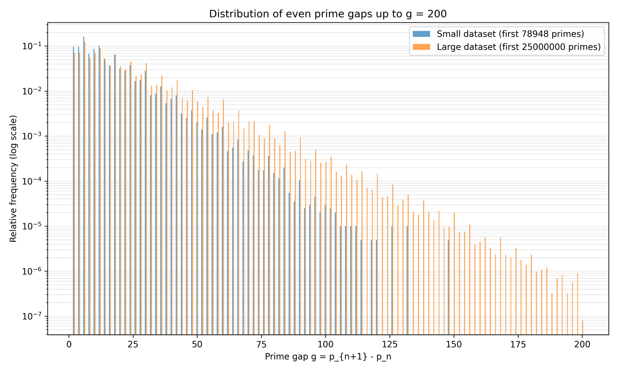
It is observed that the relative frequency of even prime gaps declines rapidly with the size of the gap g for both data sets, in such a way as to form a roughly linear downward trend on the logarithmic y-axis of Figure 1. So, there is an exponential decay in the number of larger prime gaps. The two sets of data show a repeating trend that the third even gap (g=6, 12, 18, etc.) is more frequent than the surrounding gaps. The distributions are very close in all gaps. This indicates that the behavior of the smaller generated data set is representative of the overall behavior. The distribution from the whole prime data set is clearly smoother, however, particularly for larger values of g, due to the reduced statistical noise from the larger sample size.

Empirical Gap Frequencies vs Hardy–Littlewood Weights

Finally, in Figure 2, we display some empirical frequencies and normalized Hardy–Littlewood weights for even gaps up to g = 200.

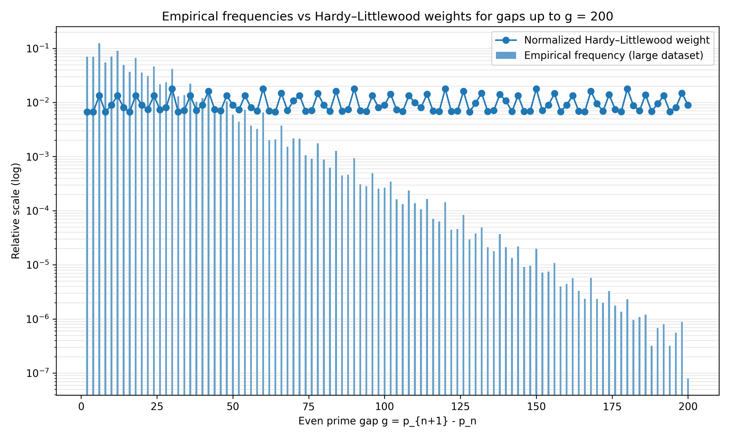
The bars show the actual relative frequencies of even gaps in a large set of numbers, and the line shows the normalized Hardy-Littlewood theoretical weights. For both quantities, there is a general trend of decreasing as the gap size g increases. Nevertheless, the Hardy-Littlewood curve shows some irregularities; there are definite peaks at certain gap values, particularly at multiples of 6 and significantly at multiples of 30.

Remarkably, the actual frequencies usually have local maxima very close to these theoretical peaks. For example, the gap g = 6 and g = 30 have much larger observed frequencies than the adjacent gaps and relative frequencies of approximately 10⁻² and 10⁻³ respectively. The Hardy-Littlewood weights are a pretty good indicator of the relative probability of the event of an even prime gap occurring, as this match shows, although the data may contain a certain amount of statistical noise, particularly for larger differences.

The same data are presented in a different format in Figure 3.

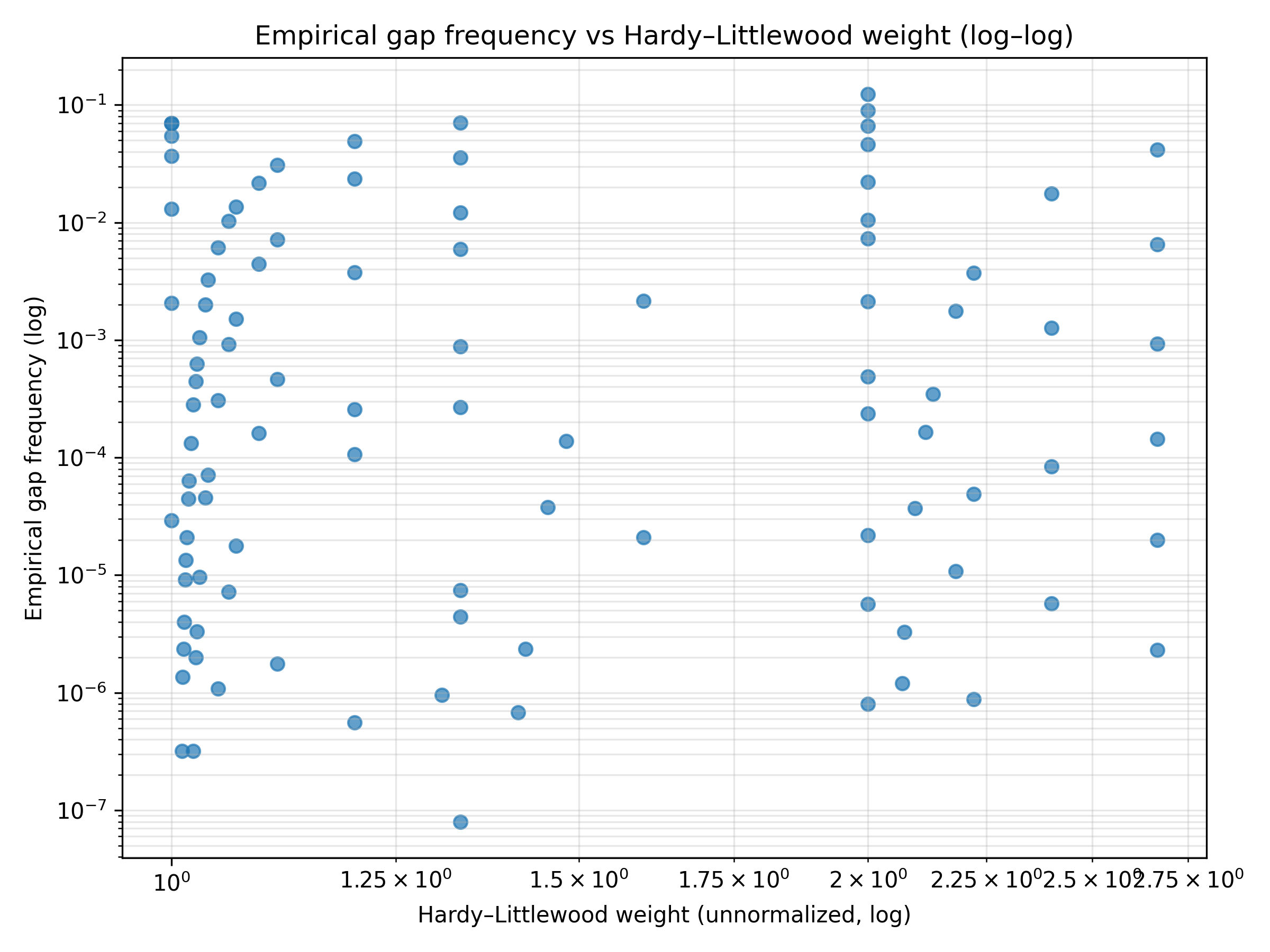
The scatter plot with the even prime gap frequencies plotted on the X-axis and the unnormalized Hardy-Littlewood weights on the Y-axis is shown in Figure 3. The points indicate one gap size each. However, the points are not grouped along a well-defined increase line, but rather, in groups that are vertically grouped denoting the different nature of the gap sizes. There is no correlation between log(weight) and log(frequency): the Pearson cor. coefficient is r = 0.0507 (p = 0.616); the Spearman rank cor. coefficient is ρ = 0.0364 (p = 0.719). For both values, the values are very close to zero and statistically insignificant, indicating that there is no global linear or monotonic correlation between the weights of Hardy–Littlewood and the frequencies in log-space. This is the expected result: If there is a near-zero Pearson r on the log transformed data, then the weights are not predicting the frequencies using a simple power law. The one shown in Figure 2 is only a local, qualitative correspondence at the arithmetically preferred gap sizes, g = 6 and g = 30, not a proportionality. The Hardy–Littlewood model is not a model of absolute size of gaps, but a model of relative ordering of a set of gap sizes.

Behaviour of the Normalized Cramér Ratio

The running maximum of the Cramér ratio R(p_n) is plotted against p_n in Figure 4.

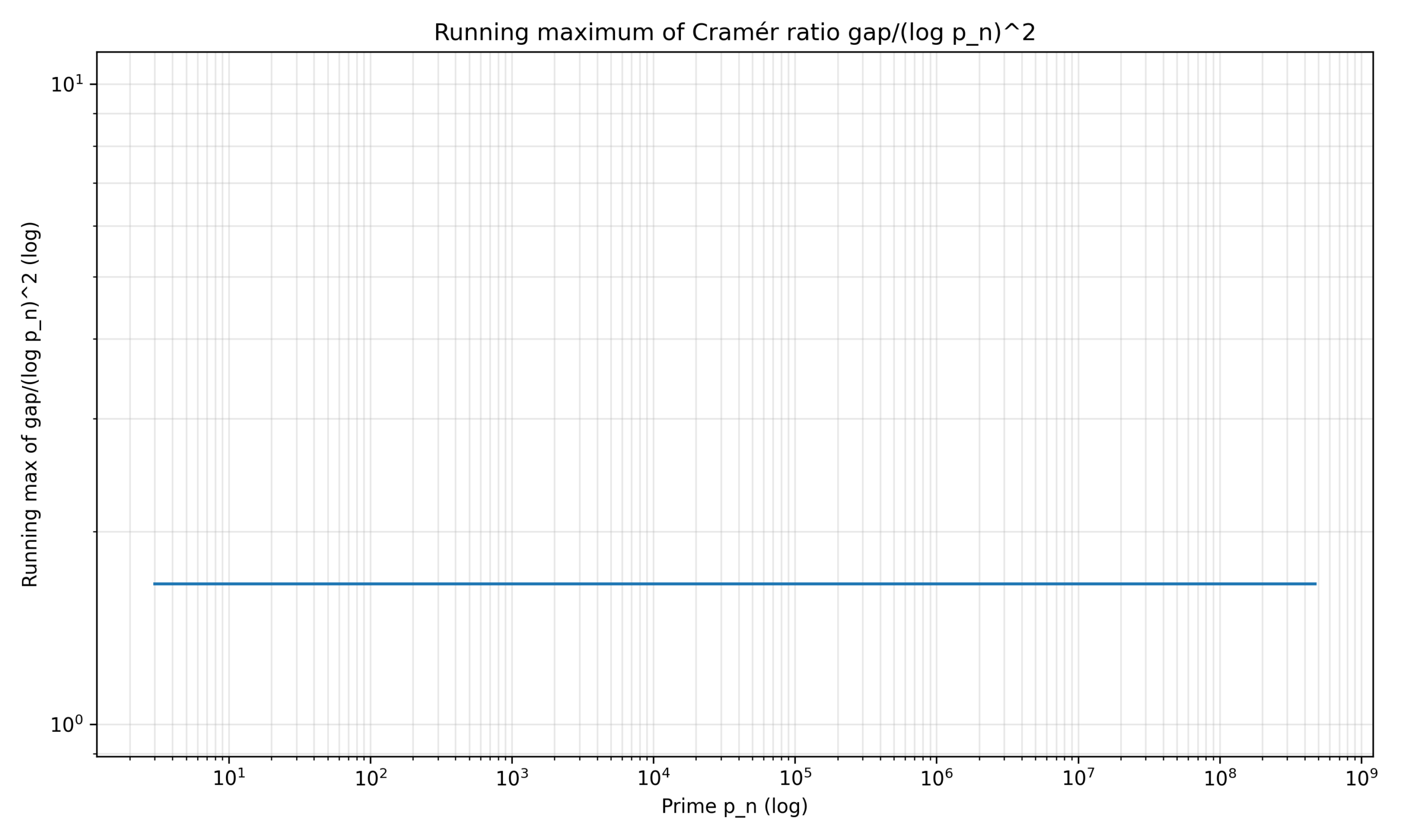
The running maximum of the normalized Cramér ratio R(p_n) is plotted against p_n on log-log scales in Figure 4. The running maximum levels out and remains almost constant over the entire range of primes computed, although there is a slight rise around the very small prime values, not visible on this scale. The graph is almost flat, suggesting that there are no substantially larger normalized gaps as p_n gets larger, up to the largest primes in consideration. The running maximum remains significantly under the Granville threshold of 2e^−γ ≈ 1.1229, marked by the red dashed line in the figure. In the range of computation studied, this is consistent with both Cramér’s original conjecture and Granville’s refinement^5,6,16; as mentioned in the Cramér’s Conjecture subsection above, data up to this scale is not able to separate the two models. Figure 5 presents the same quantity in a different way, with exceedance rates.

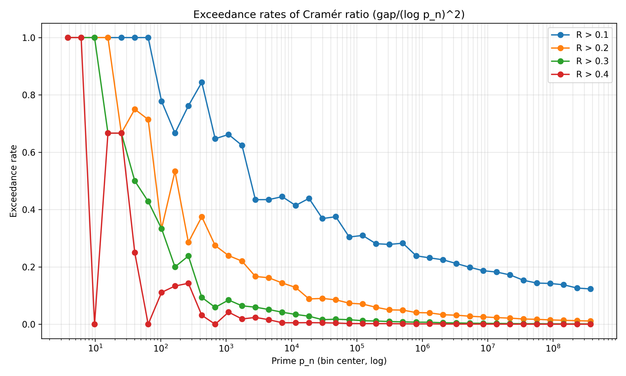
The exceedance rates for the normalized Cramér ratio R(p_n) over a number of fixed thresholds are plotted in Figure 5. These were computed in bins of the prime variable p_n, which were distributed logarithmically. For each curve, the fraction of prime gaps that have R(p_n) larger than a prescribed number, e.g., 0.1, 0.2, 0.3, 0.4, are plotted. The exceedance rates decrease with increasing p_n in comparison with the first interpretation. For example, the percentage of gaps with R(p_n) > 0.1 decreases gradually with the range. The drop is greater for higher threshold. The probability of exceedance becomes very small, even as low as 0, for large values of prime when the value is higher than 0.3 and 0.4 respectively. This trend is indicative that as p_n increases in the range of computations studied the large normalized prime gaps become less frequent. This together with the flat running maximum seen in Figure 4, indicate that there are record gaps, but that these are not more frequent relative to the (log p_n)² scale.

Residual Analysis

The residuals between the gap frequencies, as obtained from the empirical data and the normalized Hardy-Littlewood weights for even gaps up to g = 200 are displayed in Figure 6.

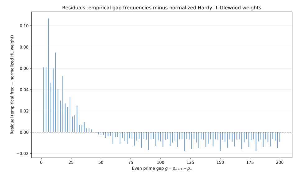
From the Figure 6, it is observed that the residuals are maximum and positive for small gaps (g ≤ 50) with the maximum deviation at g = 6 (residual = 0.107). For g > 50, residuals go through zero and become small and negative with a minimum of residual = −0.018 at g = 180. The overall standard deviation of the residuals is 0.022. The pattern is not just noise: It is characteristic in the sense that the strong positive trend at small gaps and the strong negative trend at large gaps are both systematic and indicate the limit of the single global factor λ in scaling the product of the two. However, the relative peaks are very well preserved throughout the entire range.

Discussion

This investigation looked at how prime gaps behave statistically through empirical computation and comparisons with the heuristic models of Hardy-Littlewood, and Cramér. Even prime gaps were shown in the basic way in Figures 1 and 2. The gaps are exponentially distributed on a log scale as the gap size increases, and the frequency of gaps drops off rapidly with increasing gap size. The figures exhibit a periodic pattern: gaps like 6, 12, and 18 occurred more than their close even gaps. The larger dataset looked smoother than the smaller dataset, and demonstrated how the smaller data set preserved the general shape, but with more statistical noise.

A comparison of empirical relative frequencies and unnormalized Hardy–Littlewood weights is given on a log-log scale in Figure 3. The scatter plot had the points grouped in clusters along the vertical axis by the size of a gap. log(weight) and log(frequency) had a Pearson correlation coefficient of r = 0.0507 (p = 0.616) and a Spearman rank correlation coefficient of ρ = 0.0364 (p = 0.719). Both are close to zero and not statistically significant, and illustrate no global linear or monotonic relationship in log-space. This is the expected result: the Hardy–Littlewood model does not predict a power-law proportionality between weights and frequencies, but rather governs the relative ordering of peaks at arithmetically favored gap sizes. The qualitative peak alignment seen in Figure 2 is a local, structural effect, which is predicted by the conjecture²⁴.

Figures 4 and 5 were used for the normalized Cramér ratio R(p_n) to discuss the large prime gaps. The running maximum in Figure 4 increases at very small prime values and then flattens out, seeming to be mostly flat on log-log scales over the range examined. This means that no gaps of significant size relative to the size of p_n are observed up to the largest values of p_n that have been considered. As can be seen in Figure 5, exceedance rates for higher thresholds (such as R > 0.1, 0.2, 0.3, 0.4) decrease as a function of increasing p_n. In particular, there are very few exceedances over higher thresholds and the number of large primes is very small. These results suggest that large normalized gaps are now less frequently seen than on the scale (log p_n)² in the range studied.

These findings agree with the heuristic models of Hardy–Littlewood and Cramér for the finite range on which they are based, but they do not prove them. The arithmetic structure of the gaps that is visible indicates that the distribution of gaps is not completely random, but rather is influenced by congruence conditions^23,25. In the range explored the steady behavior of the normalized Cramér ratio and the decreasing exceedance rates are consistent with Cramér’s model^6,17; as mentioned above, no distinction is possible between the Cramér and Granville models at this computational scale. These conclusions are empirical — that is, they are shown to be consistent with the theories, but do not necessarily establish them as correct.

The aims set out in the introduction have been met. The empirical distribution of even prime gaps is quantified and their relation to Hardy–Littlewood weights is checked and the growth of large gaps is considered in relation to (log p_n)². All goals were approached in both symbolized and graphical ways, and there were consistent conclusions made in both methods for each goal.

There are also some restrictions. For one, it is a limited amount of data and a very small fraction of the infinite prime sequence. The very rare events and exceptions may not show up even at this level and may easily be overlooked. In addition, the results are sensitive to several factors such as bin width, normalization and floating point precision that may introduce minor discrepancies in the numerical results without altering the general qualitative patterns.

A wider computation to larger prime ranges with more powerful resources can expand the computation, and sample more rare extreme gaps in the future. The same empirical approach could be applied to test other models, including the new versions of Cramér’s conjecture^6,17. Other data, such as distribution of gap spacing in the records or higher moment analyses, could be useful for understanding the structure of large prime gaps^{20,26,27,28,29}.

Conclusion

This research involved a study of the prime gap phenomenon over the first 25 million primes with two heuristic models. The running maximums of R(p_n) were found to be consistently below Granville’s threshold of 2e^−γ ≈ 1.1229 for the entire range computed, and the number of times that the value of R(p_n) exceeded a fixed threshold decreased with increasing p_n. Empirical gap frequencies revealed qualitative peak alignment with predicted frequencies at gap sizes that the Hardy–Littlewood conjecture predicts to be more frequent, g = 6 and g = 30, and near-zero Pearson and Spearman correlations were obtained in log space, verifying that the agreement is structural rather than globally proportional. All in all, these results are compatible with both conjectures on the finite range studied, and highlight the fact that asymptotic statements cannot be supported from computational evidence. To obtain a better understanding of the fine structure of prime gap distributions, future research on larger ranges of primes, or on using other statistical techniques like higher-moment analyses and pair-correlation methods³⁰, may be useful.

Appendix: Computational Methods and Pseudocode

All computations were performed in Python 3.11 using NumPy, Pandas, Matplotlib, SciPy, and SymPy. The full source code is provided as a supplementary file (generate_prime_gap_figures.py).

Parameters

Parameter	Value
Prime dataset	First 25,000,000 primes (PrimePages, ref 6)
Small dataset	First 200,000 primes (self-generated, p ≤ 1,000,000)
Maximum gap analyzed	g = 200
Exceedance bins	40 log-spaced bins
Cramér thresholds	R > 0.1, 0.2, 0.3, 0.4
HL scaling factor λ	≈ 6.697 × 10⁻³
Pearson r (log-log)	0.0507 (p = 0.616)
Spearman ρ (log-log)	0.0364 (p = 0.719)

Pseudocode

1. Gap computation

load primes from CSV into sorted array P
for each consecutive pair (P[n], P[n+1]):
    gap[n] = P[n+1] – P[n]

2. Normalized Cramér ratio

for each gap[n] at prime P[n]:
    R[n] = gap[n] / (ln(P[n]))²
running_max[n] = max(R[0], R[1], …, R[n])

3. Hardy–Littlewood weights and scaling

for each even gap g in 2, 4, 6, …, 200:
    k = g / 2
    w[g] = product of (p-1)/(p-2) over odd prime divisors p of k
    freq[g] = count(gap == g) / total_gaps
scaling_factor = sum(freq) / sum(w)   # = 1 / sum(w)
w_normalized[g] = w[g] * scaling_factor

4. Exceedance rates

divide primes into 40 log-spaced bins
for each bin b and threshold t in 0.1, 0.2, 0.3, 0.4:
    exceedance_rate[b][t] = count(R[n] > t in bin b) / count(primes in bin b)

5. Correlation statistics

log_w = log(w[g]) for all g where w[g] > 0 and freq[g] > 0
log_f = log(freq[g]) for same g
Pearson_r, p_value  = pearsonr(log_w, log_f)
Spearman_r, p_value = spearmanr(log_w, log_f)

References

1. G. H. Hardy, E. M. Wright. An introduction to the theory of numbers. Oxford University Press, 2008. [↩] [↩] [↩]
2. T. M. Apostol. Introduction to analytic number theory. Springer, 1976. [↩] [↩] [↩]
3. H. Davenport. Multiplicative number theory. 3rd ed. Springer, 2000. [↩] [↩] [↩]
4. H. Cramér. On the order of magnitude of the difference between consecutive prime numbers. Acta Arithmetica. Vol. 2, pg. 23–46, 1936, https://doi.org/10.4064/aa-2-1-23-46. [↩] [↩] [↩]
5. A. Granville. Harald Cramér and the distribution of prime numbers. Scandinavian Actuarial Journal. Vol. 1995, pg. 12–28, 1995, https://doi.org/10.1080/03461238.1995.10413946. [↩] [↩] [↩] [↩]
6. J. Pintz. Cramér vs. Cramér: on Cramér’s probabilistic model for primes. Functiones et Approximatio Commentarii Mathematici. Vol. 37, pg. 361–376, 2007, https://doi.org/10.7169/facm/1229619660. [↩] [↩] [↩] [↩] [↩] [↩]
7. D. A. Goldston, J. Pintz, C. Y. Y ld r m. Primes in tuples I. Annals of Mathematics. Vol. 170, pg. 819–862, 2009, https://doi.org/10.4007/annals.2009.170.819. [↩]
8. Y. Zhang. Bounded gaps between primes. Annals of Mathematics. Vol. 179, pg. 1121–1174, 2014, https://doi.org/10.4007/annals.2014.179.3.7. [↩]
9. J. Maynard. Small gaps between primes. Annals of Mathematics. Vol. 181, pg. 383–413, 2015, https://doi.org/10.4007/annals.2015.181.1.7. [↩]
10. P. Erdős. The difference of consecutive primes. Duke Mathematical Journal. Vol. 6, pg. 438–441, 1940, https://doi.org/10.1215/S0012-7094-40-00635-4. [↩]
11. M. Wolf. Nearest-neighbor-spacing distribution of prime numbers and quantum chaos. Physical Review E. Vol. 89, pg. 022922, 2014, https://doi.org/10.1103/PhysRevE.89.022922. [↩]
12. C. K. Caldwell. The prime pages: prime number research, records and resources. https://primes.utm.edu, 2025. [↩] [↩]
13. A. E. Ingham. On the difference between consecutive primes. Quarterly Journal of Mathematics. Vol. 8, pg. 255–266, 1937, https://doi.org/10.1093/qmath/os-8.1.255. [↩]
14. R. C. Baker, G. Harman, J. Pintz. The difference between consecutive primes, II. Proceedings of the London Mathematical Society. Vol. 83, pg. 532–562, 2001, https://doi.org/10.1112/plms/83.3.532. [↩]
15. H. Maier. Primes in short intervals. Michigan Mathematical Journal. Vol. 32, pg. 221–225, 1985, https://doi.org/10.1307/mmj/1029003189. [↩]
16. A. Granville. Different approaches to the distribution of primes. Milan Journal of Mathematics. Vol. 78, pg. 65–84, 2010, https://doi.org/10.1007/s00032-010-0122-7. [↩] [↩]
17. W. D. Banks, K. Ford, T. Tao. Large prime gaps and probabilistic models. Inventiones Mathematicae. Vol. 233, pg. 1471–1518, 2023, https://doi.org/10.1007/s00222-023-01199-0. [↩] [↩] [↩]
18. K. Ford, B. Green, S. Konyagin, T. Tao. Large gaps between consecutive prime numbers. Annals of Mathematics. Vol. 183, pg. 935–974, 2016, https://doi.org/10.4007/annals.2016.183.3.4. [↩]
19. K. Ford, B. Green, S. Konyagin, J. Maynard, T. Tao. Long gaps between primes. Journal of the American Mathematical Society. Vol. 31, pg. 65–105, 2018, https://doi.org/10.1090/jams/876. [↩]
20. T. Oliveira e Silva, S. Herzog, S. Pardi. Empirical verification of the even Goldbach conjecture and computation of prime gaps up to 4 10¹⁸. Mathematics of Computation. Vol. 83, pg. 2033–2060, 2014, https://doi.org/10.1090/S0025-5718-2013-02787-1. [↩] [↩]
21. G. H. Hardy, J. E. Littlewood. Some problems of `Partitio numerorum’; III: On the expression of a number as a sum of primes. Acta Mathematica. Vol. 44, pg. 1–70, 1923, https://doi.org/10.1007/BF02403921. [↩] [↩] [↩] [↩] [↩] [↩]
22. H. L. Montgomery, R. C. Vaughan. Multiplicative number theory I: Classical theory. Cambridge University Press, 2007. [↩] [↩] [↩] [↩] [↩] [↩] [↩]
23. A. Selberg. On the normal density of primes in short intervals, and the difference between consecutive primes. Archiv for Mathematik og Naturvidenskab. Vol. 47, pg. 87–105, 1943. [↩] [↩]
24. R. J. Lemke Oliver, K. Soundararajan. Unexpected biases in the distribution of consecutive primes. Proceedings of the National Academy of Sciences. Vol. 113, pg. E4446–E4454, 2016, https://doi.org/10.1073/pnas.1605366113. [↩]
25. K. Soundararajan. The distribution of prime numbers. Equidistribution in Number Theory, An Introduction, NATO Science Series II. Vol. 237, pg. 59–83, 2007, https://doi.org/10.1007/978-1-4020-5404-4_5. [↩]
26. A. Kourbatov, M. Wolf. Predicting maximal gaps in sets of primes. Mathematics. Vol. 7, no. 5, pg. 400, 2019, https://doi.org/10.3390/math7050400. [↩]
27. A. Kourbatov, M. Wolf. On the first occurrences of gaps between primes in a residue class. Journal of Integer Sequences. Vol. 23, Article 20.9.3, 2020, https://cs.uwaterloo.ca/journals/JIS/VOL23/Wolf/wolf2.html. [↩]
28. T. R. Nicely. New maximal prime gaps and first occurrences. Mathematics of Computation. Vol. 68, pg. 1311–1315, 1999, https://doi.org/10.1090/S0025-5718-99-01065-0. [↩]
29. J. E. Cohen. Gaps between consecutive primes and the exponential distribution. Experimental Mathematics. Vol. 34, pg. 1–20, 2024, https://doi.org/10.1080/10586458.2024.2362348. [↩]
30. H. L. Montgomery. The pair correlation of zeros of the zeta function. Analytic Number Theory (Proc. Sympos. Pure Math., Vol. XXIV), American Mathematical Society, pg. 181–193, 1973. [↩]