
Abstract
Written music leaves much room for interpretation. A marking such as “cresc. poco a poco” tells musicians to grow gradually louder, but two performers will change volume at different rates. We hypothesized that professional musicians would interpret such a marking more similarly to each other than youth musicians would, potentially due to hearing other professional musicians interpret the same passage. To quantify this, we analyzed the timpani crescendo in the Act IV No. 29 Finale of Tchaikovsky’s Swan Lake in 16 recordings found on YouTube, eight by professional orchestras and eight by youth orchestras. A Python script extracted the root-mean-square (RMS) amplitude of each recording every 10 ms, and a 3-second window beginning at the start of the crescendo was kept. Each crescendo was treated as a vector, and every pair of recordings within a group was compared using cosine similarity, with Pearson correlation as a second measure. Mean cosine similarity was .9083 (SD = .1104) across the 28 professional pairs and .8101 (SD = .1363) across the 28 youth pairs (Welch’s t test, p = .005; Mann–Whitney U test, p < .001), and Pearson correlation showed the same difference. Within this exploratory sample, professional crescendos were significantly more similar to each other than youth crescendos. The result concerns only the amplitude trajectory of one short passage and does not describe musical interpretation as a whole.
Keywords: Interpretation, Crescendo, Statistics, Interpretive Similarity, Time-Based Analysis
Introduction
Converting sheet music (or MIDI, etc.) into sound is the most basic description of what musicians do. However, many aspects of music-making are left to the musician to interpret. Expert performers shape tempo, timing, dynamics, articulation, and other parameters in ways that the score does not prescribe1, and different performances of the same composition can vary considerably in these parameters2. Lerch et al. note that tempo markings are frequently treated as suggestions, whereas dynamics are often absent from the score or only roughly defined, and they survey the various ways interpretation influences music-making3. Gabrielsson’s review of performance research shows that the measurement of such performance parameters has been the largest area of empirical work on music performance4.
Dynamics are one of the main tools of this interpretation. Juslin showed that professional guitarists communicated emotions through acoustic cues such as tempo, sound level, and articulation, and that listeners relied on the same cues to recognize the intended emotion5. Structural features of the music matter as well: in Bach’s Well-Tempered Clavier, attack rate, mode, and pitch height guide listeners’ judgments of emotional valence, and attack rate also guides judgments of intensity6. Listeners follow loudness changes continuously, and Geringer found that crescendos are judged as larger changes than decrescendos7, whereas Farbood and Upham showed that dynamics are among the features that shape listeners’ sense of musical tension8. The meaning of a dynamic marking is itself relative. In recordings of Chopin’s Mazurkas, Kosta et al. found that the loudness corresponding to a marking depends strongly on the context in which it appears9,10, and they applied change-point detection to locate changes in dynamics within recorded performances11. Cheng and Chew found that loudness was a more consistent indicator of phrasing than tempo in performances of unaccompanied Bach for solo violin12.
Several studies have measured how performers differ. Repp analyzed expressive timing in 115 commercial recordings of the opening of Chopin’s Etude in E major and found a small number of shared timing strategies alongside individual variation13. Fabian and Schubert compared dotting, articulation, and tempo in 34 commercial recordings of one of Bach’s Goldberg Variations14, and Schubert and Fabian identified the dimensions listeners use to judge baroque performances15. Computational models attempt to capture such regularities in mathematical or algorithmic form16. Widmer used machine learning to discover simple, general rules of expressive performance in complex performance data17, and Cancino-Chacón et al. compared linear and non-linear models that predict expressive dynamics in piano and orchestral music from features of the score18. Lerch et al. point out the difficulty of matching the differences that computational models find to concepts such as “expressiveness”3. Other work has found it difficult to obtain large datasets: Cancino-Chacón et al. note that many large-scale datasets are not publicly available, restricting opportunities to test and fine-tune computational models1, and creating a new multitrack dataset of classical ensemble performances requires careful synchronization of separately recorded parts19.
Judging performance is itself difficult. McPherson and Thompson describe the many factors that affect a judge’s assessment of a performance20. Thompson and Williamon found only moderate agreement between experienced evaluators21, and Wesolowski et al. showed that raters differ in how precisely they apply scoring criteria22. Visual factors also play a role: high school band students rated the same ensemble recordings as more or less expressive depending on the conductor’s facial expression23. Automatic assessment offers one alternative; Wu and Lerch, for example, used learned audio features to assess student percussion performances24. Together, these studies point to an overarching difficulty in creating computational models that can measure certain properties across a whole performance, which is partly linked to the lack of an easily computable association between performance details and audience perception. Thus, we explored a different avenue that could be more applicable to computational models: a bottom-up approach that analyzes one of the smallest interpretive decisions to quantify similarity.
There are reasons to expect professional musicians to play more alike. Expression is not random: Clarke found that pianists imitated real expressive performances more accurately and stably than versions in which the link between musical structure and expression had been disrupted, which suggests that expression is generated from the performer’s understanding of musical structure25. Sloboda found significant agreement among pianists on the position and direction of expressive variation, and the more experienced players made greater use of it26. Listeners also appear to value a shared norm: Repp found that a performance created by averaging several student performances was rated second highest in quality27, and Wolf et al. successfully replicated this study with listeners in Germany and Taiwan28. Professional orchestral musicians typically have extensive training, and they hear many recordings and performances by other professionals. We therefore reasoned that professionals may be familiar with, and unconsciously match, other professionals’ styles of play, so that they converge on a common interpretation of a passage, whereas youth musicians, with less training and exposure, may vary more.
We analyzed a basic part of music, the crescendo, to understand how classical musicians interpret sheet music. A crescendo, in its most basic form, is simply an increase in the volume of play from a lower level to a higher level. However, crescendos are typically designated only by their start and end volumes and thus leave room for interpretation. Therefore, we sampled online recordings of performances and used the progression of volume, measured as RMS amplitude, over a crescendo to measure the similarity between interpretations. We hypothesized that professional musicians would play more similarly to each other than youth orchestra members would. This study measures only one narrow acoustic aspect of interpretation, the amplitude trajectory of a single crescendo. It does not measure interpretation as a whole, which also includes timing, phrasing, articulation, balance, timbre, vibrato, and accentuation.
Methods
Research Design
This is an exploratory observational study that analyzes a small aspect of interpretation to determine whether measuring sound amplitude over time is an effective way to compare interpretations.
Participants or Sample
The timpani crescendo in the Act IV No. 29 Finale of Tchaikovsky’s Swan Lake was sampled for our analysis. This crescendo was chosen because it isolates the effect of a single dynamic marking: few instruments are playing relative to a typical point in an orchestral performance, all the instruments involved have the same dynamic markings, and the passage grows from very quiet to very loud. Eight professional and eight youth orchestra performances were chosen by hand from a YouTube search for the piece (Table 1). A professional orchestra was defined as an orchestra whose musicians are paid for their work and that performs commercially on a repeated basis; the youth group consisted of school and youth orchestras. A recording was included if it was a performance of the same passage and the start of the timpani crescendo could be located. One professional recording was excluded because the start of the crescendo could not be found. The recordings were not simply the first eight of each group that satisfied these criteria, and each recording was selected before its crescendo was heard. However, because of the way YouTube ranks and recommends videos, the sample cannot be considered a random selection of all Swan Lake Finale performances, and factors such as popularity restrict the generalizability of our results.
| ID | Group | Orchestra | Conductor | Source | Start (min:s) |
| P1 | Professional | American Ballet Theater | Not named | https://www.youtube.com/watch?v=JI7AsZGnyi4 | 1:46 |
| P2 | Professional | Royal Liverpool Philharmonic Orchestra | Not named | https://www.youtube.com/watch?v=C7c1b931zvk | 3:05 |
| P3 | Professional | London Symphony Orchestra | André Previn | https://www.youtube.com/watch?v=V2u-QOOzqBM | 3:20 |
| P4 | Professional | Montreal Symphony Orchestra | Charles Dutoit | https://www.youtube.com/watch?v=5BpzS1m6gc0 | 3:20 |
| P5 | Professional | Queensland Symphony Orchestra | Not named | https://www.youtube.com/watch?v=EMotDEOEKzA | 0:02 |
| P6 | Professional | Orchestre symphonique de Montréal | Not named | https://www.youtube.com/watch?v=yE2jFTxLc1Y | 1:53 |
| P7 | Professional | Boston Symphony | Seiji Ozawa | https://www.youtube.com/watch?v=rH8jj6XIvl8 | 2:51 |
| P8 | Professional | Philharmonia Orchestra | Not named | https://www.youtube.com/watch?v=r0f4vYJMbn0 | 3:01 |
| Y1 | Youth | Martin High School Symphony Orchestra | Not named | https://www.youtube.com/watch?v=o8TVBwFU_Iw | 2:58 |
| Y2 | Youth | Highland High Symphony | Not named | https://www.youtube.com/watch?v=Wog6i_R7UOQ | 3:32 |
| Y3 | Youth | Glenbrook HS Symphony Orchestra | Not named | https://www.youtube.com/watch?v=PEKRENMIQhw | 1:56 |
| Y4 | Youth | Kuang Jen High School Orchestra | Not named | https://www.youtube.com/watch?v=V9M_OGK08_c | 34:38 |
| Y5 | Youth | Takanawadai High School | Not named | https://www.youtube.com/watch?v=Iza-ELVWPB4 | 6:18 |
| Y6 | Youth | Tokyo Junior Orchestra Society | Not named | https://www.youtube.com/watch?v=WoHHlEyJo9Q | 1:54 |
| Y7 | Youth | Orchestra Wawon | Not named | https://www.youtube.com/watch?v=79I1wqO3rOw | 3:08 |
| Y8 | Youth | Yilan Youth Wind Orchestra | Not named | https://www.youtube.com/watch?v=-0f2KJzqSeg | 0:59 |
Variables and Measurements
The measured variable was the root-mean-square (RMS) amplitude of the audio, extracted every 10 ms. For each frame of N digital sample values xᵢ (i = 1, …, N), the RMS value is the square root of the mean of the squared amplitudes:
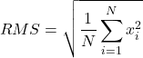
RMS is a relative amplitude measure on the scale of the recording’s digital samples. It is not expressed in decibels and is not a calibrated sound pressure level, so the RMS curves of different recordings can be compared in shape but not in absolute loudness.
Procedure
The analysis followed five steps.
Step 1: The start time of the timpani crescendo was marked manually in each of the 16 recordings, at the same point of the Finale (Table 1).
Step 2: A Python script retrieved the RMS amplitude of each recording every 10 ms (220 samples) with a frame length of 2048 samples, resampled to 22,050 Hz, and merged into a mono channel sound, along with YouTube’s original bit depth for each video (which varied depending on upload).
Step 3: The leading silent and decreasing values of each RMS series were trimmed to give a precise start point for each crescendo.
Step 4: Starting from the first increasing value, 3 seconds of RMS data were kept from each recording, which is enough to contain the timpani crescendo. No smoothing, rescaling, or interpolation was applied; all analyses used the raw RMS values. For a visual comparison only, a wider 8-second window, which includes other instruments entering after the timpani, was also extracted.
Step 5: Python was used to compute the pairwise similarity of the 3-second RMS vectors and to compare the groups statistically, as described below.
Data Analysis
To determine whether two crescendos were interpreted similarly or differently, we turned to linear algebra. The progression of RMS amplitude over the course of a crescendo can be considered a many-dimensional vector, with one dimension for each 10 ms frame. The dot product of two vectors equals the product of their magnitudes multiplied by the cosine of the angle between them, so it can be used to calculate that cosine as a measure of similarity. Similarity was therefore measured with cosine similarity:

where A and B are the RMS vectors of two recordings and the sums run over all frames in the 3-second window. A value of 1 means that A and B have the same shape up to a scaling factor, and 0 means that they are unrelated (they form a right angle). Because RMS values are never negative, cosine similarity here lies between 0 and 1. We chose cosine similarity because it disregards differences in overall level between recordings, which depend largely on recording conditions rather than on interpretation, and compares only the shape of the crescendo. As a second measure, we used the Pearson correlation coefficient r, which is the cosine similarity of the two vectors after each has had its mean subtracted:
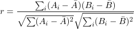
Because all RMS values are positive, any two crescendos share a large positive component, which keeps their cosine similarity high. Pearson correlation removes each vector’s mean and therefore compares only how the two curves vary around their own average level.
Similarity was computed for every pair of recordings within each group: 28 pairs within the professional group and 28 pairs within the youth group. For Pearson correlation, the 64 pairs between the groups were also computed. The mean pairwise similarity of each group was then calculated. We tested whether the mean within-professional similarity was significantly greater than the mean between-group similarity using a permutation test. Then, we tested whether the mean within-professional similarity was significantly higher than the mean within-youth similarity. For cosine similarity, the two groups of pairwise values were compared using a permutation test, Welch’s t test, and the Mann–Whitney U test, all one-sided. For Pearson correlation, the hypothesis that professional similarity is greater than youth similarity was tested with a one-sided Mann–Whitney U test. As an informal check, we listened to the pairs with the highest and lowest similarity under each measure to see whether they also sounded the most and least alike; this was true for cosine similarity but not for Pearson correlation. The analysis code is given in the Appendix, and the raw and processed RMS data are provided as supplementary material.
We used cosine similarity because it is used in areas such as machine learning to group ideas based on qualitative similarity, and it is relatively resistant to noise in high dimensions compared with metrics such as Euclidean distance. Also, it discards magnitude, which is not very meaningful in our analysis due to recording differences and post-recording sound transformations before our analysis. We used Pearson correlation because it measures how much one sequence can be predicted from the other and therefore measures whether the two samples progress similarly over time.
Ethical Considerations
The study used only publicly available recordings and involved no human participants or animal subjects, so institutional review board (IRB) approval was not required.
Results
Figures 1 and 2 show the 3-second RMS trajectories of the timpani crescendo for the professional and youth recordings. In the two line charts, the professional crescendos form a qualitatively tighter band than the youth performances.
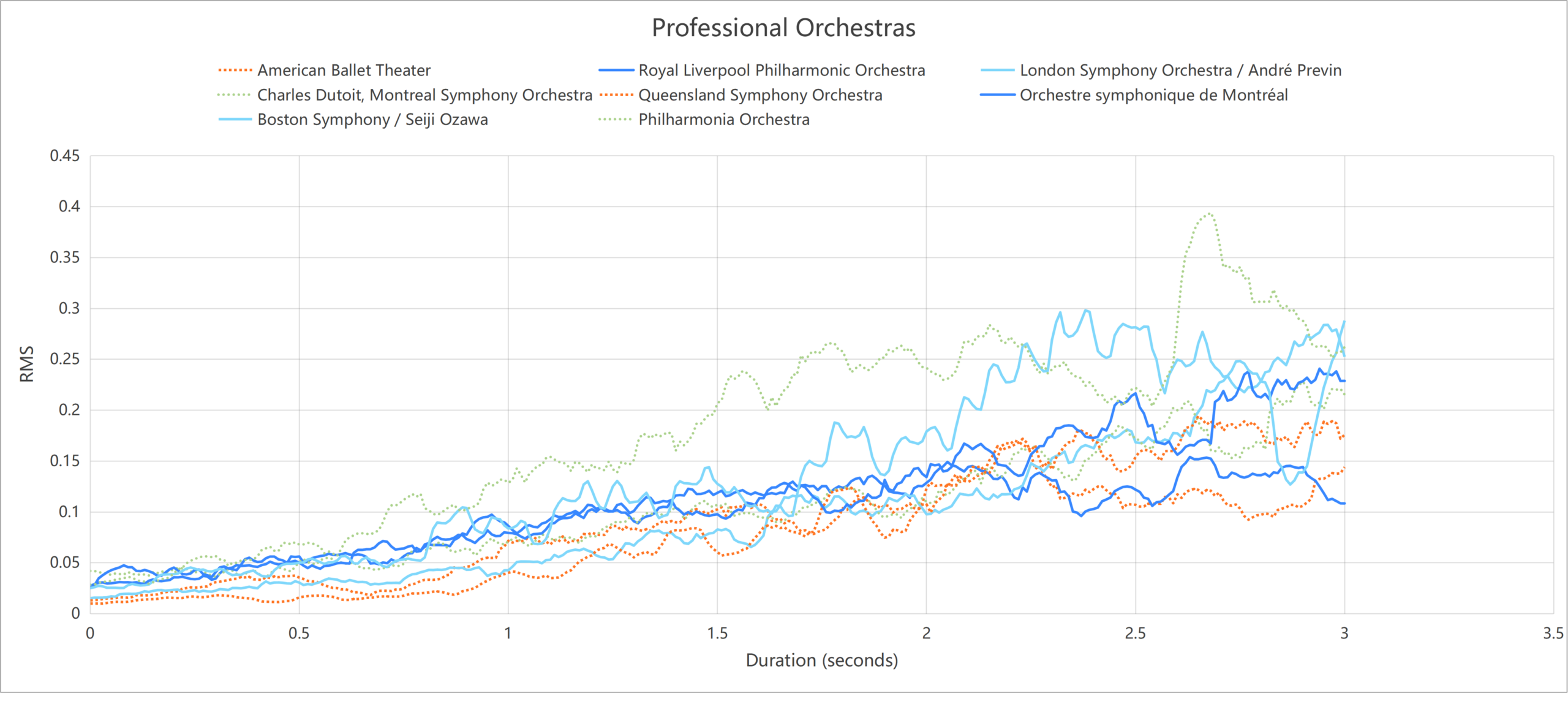
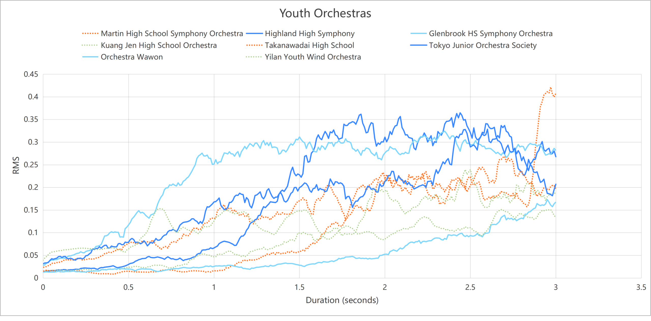
Table 2 summarizes the pairwise similarities. The difference between average within-professional similarity and average between-group similarity was 0.018718. Using a null hypothesis that labels were irrelevant and that this result occurred due to random chance, this difference was recomputed for each permutation of the labels “professional” and “youth”. The proportion of permutations with an equal or larger difference was 538/12870 = 0.041803, giving a permutation p-value of 0.041803 < 0.05, indicating significantly greater similarity within the professional group compared to between the two groups.
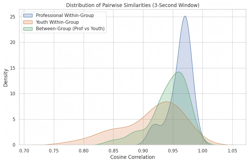
In addition, there was a larger difference between the average pairwise distances within the professional group and within the youth group. The mean cosine similarity of the 28 professional pairs was .9622 (SD = .0185), and that of the 28 youth pairs was .9139 (SD = .0490), an absolute difference of .0483. There was significantly greater than 0 difference according to the permutation test, with a permutation p-value of 49/12870 = 0.003807. The difference was significant with both Welch’s t test (p = .0025) and the Mann–Whitney U test (p < .001). Pearson correlation gave the same result: the mean within-professional correlation was .8707 (SD = .0599), the mean within-youth correlation was .7056 (SD = .1671), and the difference was significant (U = 550, p = .005). The mean between-group correlation, .7981 (SD = .1301), lay between the two within-group values. Figure 3 shows the distribution of the pairwise Pearson correlations for each comparison.
| Measure | Within professional (28 pairs) | Within youth (28 pairs) | Between groups (64 pairs) | Test of professional vs. youth |
| Cosine similarity | .9622 ± .0185 | .9139 ± .0490 | .9434 ± .0308 | Permutation test, p = 0.0846; Welch’s t test, p = .0025; Mann–Whitney U test, p < .001 |
| Pearson r | .8707 ± .0599 | .7056 ± .1671 | .7981 ± .1301 | Mann–Whitney U = 550, p = .005 |
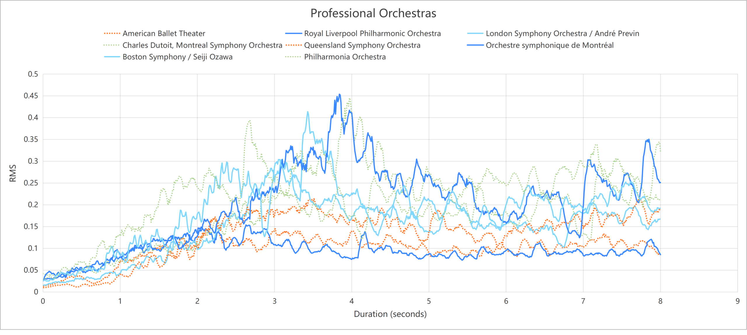
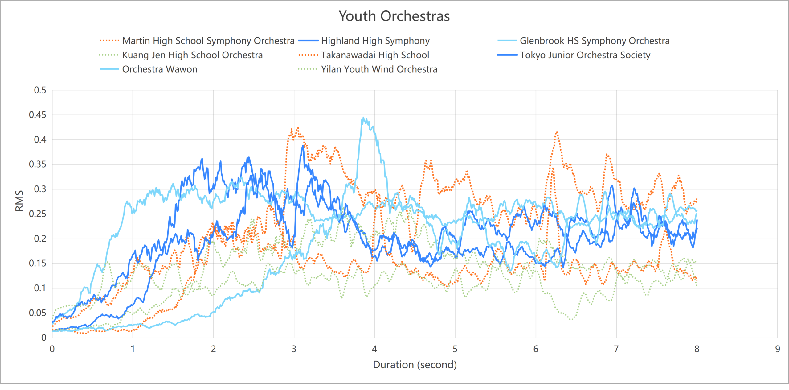
When the window was widened to 8 seconds to include the other instruments that enter after the timpani crescendo, the youth orchestras’ lines again appeared qualitatively more erratic than the professional orchestras’ lines, which stayed closer to a common pattern (Figures 4 and 5).
Discussion
In this sample, the RMS amplitude trajectories of the professional orchestras’ timpani crescendos were significantly more similar to each other than those of the youth orchestras. Cosine similarity and Pearson correlation showed the same difference, and the mean between-group correlation fell between the two within-group means. This is consistent with our hypothesis that professional musicians converge on a shared interpretation of a passage, and with earlier findings that expressive performance is closely tied to musical structure and can be imitated25 and that listeners favor performances close to the average27. The result should be read narrowly: it is a limited analysis of the amplitude changes in one short crescendo, not of the entire interpretation of a score.
The study makes two contributions that should not be equated. The methodological contribution is a clear, quantitative way to measure similarity in small interpretive decisions, such as a single short crescendo or decrescendo, which does not require large datasets. The empirical contribution, evidence that professional orchestras play this crescendo more alike than youth orchestras, rests on a small, non-random sample and should be treated as exploratory. The agreement between the two similarity measures is relevant to the method: because all RMS values are positive, cosine similarity is high for almost any pair of crescendos, whereas Pearson correlation removes this shared positive level. That both measures show the same group difference suggests the result is not simply a by-product of the cosine measure.
Factors other than training could also contribute to the difference. Professional orchestras may be more familiar with this repertoire, and an orchestra’s own traditions and its conductor shape how a passage is played; conductors also influence how expressive an ensemble is perceived to be23. Recording technology, room acoustics, and microphone placement differ between commercial recordings and school concert videos and can change the measured RMS curve. Differences in instrumentation and ensemble size, for example between a wind orchestra and a full symphony orchestra, may also affect the sound of the passage.
Our sample size was small, which reduced the power of our analysis. In addition, selection bias introduced by the selection process restricts our results regarding similarity to our 16-performance sample. The recording environments varied widely, only one passage of one work was studied, and only the timpani crescendo was analyzed. Our definition of professional status rests on paid, repeated commercial performance and does not account for individual players’ training or experience. The similarity measures were also not validated against synthetic crescendos with known differences. The informal listening check described in the Methods was subjective and is not a substitute for formal validation.
We also found that crescendo shapes varied noticeably, especially among the youth orchestras, likely because dynamic markings are relatively vague compared to rhythmic or pitch markings3. Our method of turning lists of data points into graphs could be used to easily turn audio data into visual data, in which we found it easier to spot detailed patterns. Although the method is constrained to amplitude data, pairing it with a way to handle differences in absolute volume between performances and sections could allow it to be used on longer, more complicated sections.
Future studies could use a larger and more balanced sample, several musical excerpts, several instruments, a standardized recording environment, and independent assessments of musicians’ skill, which would make it easier to test the hypothesis. The comparison metric could also be applied to other samples, for example piano performances or performances from different eras, to quantify the relative stability or change of interpretation of a specific indication to change volume. Our methods could also be applied wherever too few data are available to tune a more complicated model.
Appendix
Appendix A Python code for Retrieving RMS
import os
import subprocess
import pandas as pd
import numpy as np
import librosa
import yt_dlp

from scipy.spatial.distance import cosine

from scipy import stats

def clean_leading_trajectory(series):

    values = series.dropna().values

    if len(values) == 0:

        return series

    # Step 1: Find first index within [0.01, 0.1]

    start_idx = 0

    while start_idx < len(values):

        val = values[start_idx]

        if 0.01 <= val <= 0.1:

            break

        start_idx += 1

    if start_idx >= len(values):

        return pd.Series(np.nan, index=series.index)

    # Step 2: From start_idx, remove any leading decreasing data

    curr_idx = start_idx

    while curr_idx < len(values) - 1:

        if values[curr_idx + 1] >= values[curr_idx]:

            break

        curr_idx += 1

    trimmed_values = values[curr_idx:]

    new_values = np.pad(trimmed_values, (0, len(series) - len(trimmed_values)), 'constant', constant_values=np.nan)

    return pd.Series(new_values, index=series.index)

def parse_time(t_str):

    """Converts spreadsheet time string into total seconds."""

    if pd.isna(t_str):

        return 0

    t_str = str(t_str).strip().replace("''", "'").replace('“', '"').replace('‘', "'").replace('"', '')

    if "'" in t_str:

        parts = t_str.split("'")

        mins = int(parts[0]) if parts[0] != '' else 0

        secs = int(parts[1]) if len(parts) > 1 and parts[1] != '' else 0

        return mins * 60 + secs

    elif t_str.isdigit():

        return int(t_str)

    return 0

def get_real_rms_stream(url, start_sec, duration=10, sr=22050, hop_length=220):

    """Extracts the exact audio stream segment into memory via an ffmpeg pipe and computes RMS."""

    ydl_opts = {

        'format': 'bestaudio/best',

        'quiet': True,

        'no_warnings': True,

        'http_headers': {

            'User-Agent': 'Mozilla/5.0 (Windows NT 10.0; Win64; x64) AppleWebKit/537.36 (KHTML, like Gecko) Chrome/120.0.0.0 Safari/537.36'

        }

    }

    with yt_dlp.YoutubeDL(ydl_opts) as ydl:

        info = ydl.extract_info(url, download=False)

        stream_url = info['url']

    ffmpeg_cmd = [

        'ffmpeg', '-ss', str(start_sec), '-i', stream_url, '-t', str(duration + 2),

        '-f', 'f32le', '-acodec', 'pcm_f32le', '-ar', str(sr), '-ac', '1', '-loglevel', 'panic', '-'

    ]

    process = subprocess.Popen(ffmpeg_cmd, stdout=subprocess.PIPE, stderr=subprocess.PIPE)

    stdout_data, _ = process.communicate()

    y = np.frombuffer(stdout_data, dtype=np.float32)

    if len(y) == 0:

        raise ValueError("Empty audio stream returned")

    yt, index = librosa.effects.trim(y, top_db=30)

    start_sample = index[0]

    end_sample = start_sample + int(duration * sr)

    y_trimmed = y[start_sample:end_sample]

    if len(y_trimmed) < int(duration * sr):

        padding = int(duration * sr) - len(y_trimmed)

        y_trimmed = np.pad(y_trimmed, (0, padding), 'constant')

    rms = librosa.feature.rms(y=y_trimmed, hop_length=hop_length)[0]

    return rms

def preprocess_increasing_beginning(df):

    """Filters each column from the first row downwards: if a value decreases, we discard it and shift up, repeating until the column starts with non-decreasing values."""

    filtered_df = df.copy()

    orchestra_cols = [col for col in filtered_df.columns if col != 'Frame_Index']

    for col in orchestra_cols:

        vals = filtered_df[col].dropna().tolist()

        # While the first element is greater than the second, remove the first element to make it increasing from the start

        while len(vals) > 1 and vals[0] > vals[1]:

            vals.pop(0)

        # Re-pad or truncate to match original DataFrame row index structure

        if len(vals) < len(filtered_df):

            vals = vals + [0.0] * (len(filtered_df) - len(vals))

        else:

            vals = vals[:len(filtered_df)]

        filtered_df[col] = vals

    return filtered_df

def main():

    excel_file = 'Swan-Lake-Finale-list.xlsx'

    if not os.path.exists(excel_file):

        print(f"Error: Master list '{excel_file}' not found.")

        return

    xls = pd.ExcelFile(excel_file)

    groups = {'professional': [], 'youth': []}

    # 1. Processing and Streaming Audio into memory

    for sheet_name in xls.sheet_names:

        df_sheet = pd.read_excel(excel_file, sheet_name=sheet_name)

        sheet_lower = sheet_name.lower()

        if 'pro' in sheet_lower or 'expert' in sheet_lower:

            group_key = 'professional'

        elif 'youth' in sheet_lower or 'student' in sheet_lower or 'junior' in sheet_lower:

            group_key = 'youth'

        else:

            group_key = 'professional' if '1' in sheet_name or len(groups['professional']) < 8 else 'youth'

        print(f"\n--- Streaming: {group_key.upper()} ({sheet_name}) ---")

        count = 0

        for idx, row in df_sheet.iterrows():

            if count >= 8:

                break

            if pd.notna(row.iloc[0]):

                name = str(row.iloc[1]).strip().replace('\n', ' ')

                url = row.iloc[2]

                time_str = row.iloc[3]

                if pd.isna(url):

                    continue

                start_sec = parse_time(time_str)

                print(f"[{group_key.upper()}] Extracting RMS: {name}...")

                try:

                    rms = get_real_rms_stream(url, start_sec)

                    groups[group_key].append({'name': name, 'rms': rms})

                    count += 1

                except Exception as e:

                    print(f" -> Failed: {e}")

    # 2. Save combined raw RMS profiles

    for group_name, output_file in [('professional', 'professional_RMS_Data.xlsx'), ('youth', 'Youth_RMS_Data.xlsx')]:

        members = groups[group_name]

        if members:

            combined_dict = {}

            max_len = max(len(m['rms']) for m in members)

            combined_dict['Frame_Index'] = list(range(max_len))

            for m in members:

                vals = m['rms']

                if len(vals) < max_len:

                    vals = np.pad(vals, (0, max_len - len(vals)), 'constant')

                elif len(vals) > max_len:

                    vals = vals[:max_len]

                combined_dict[m['name']] = vals

            df_combined = pd.DataFrame(combined_dict)

            with pd.ExcelWriter(output_file) as writer:

                df_combined.to_excel(writer, sheet_name='Raw_RMS_Profiles', index=False)

            print(f"Successfully saved raw trajectories to '{output_file}'!")

if __name__ == '__main__':

    main()
Appendix B Core Statistics Analysis Python Code
import pandas as pd
import numpy as np
from scipy.stats import ttest_ind, mannwhitneyu
import seaborn as sns
import matplotlib.pyplot as plt

def run_analysis(prof_path='/content/Professional_RMS_Data.xlsx', youth_path='/content/Youth_RMS_Data.xlsx'):

    # 1. Load the data

    print("Loading data...")

    prof_df = pd.read_excel(prof_path)

    youth_df = pd.read_excel(youth_path)

    print("Professional shape:", prof_df.shape)

    print("Youth shape:", youth_df.shape)

    # Helper to clean and calculate similarities

    def compute_pairwise_similarities(df):

        numeric_df = df.select_dtypes(include=[np.number]).dropna()

        data = numeric_df.values.T  # Shape: (orchestras, features)

        corr_matrix = np.corrcoef(data)

        triu_indices = np.triu_indices_from(corr_matrix, k=1)

        similarities = corr_matrix[triu_indices]

        return corr_matrix, similarities

    # 2. Compute within-group similarities

    prof_corr, prof_sims = compute_pairwise_similarities(prof_df)

    youth_corr, youth_sims = compute_pairwise_similarities(youth_df)

    print(f"\nProfessional Within-Group Similarity (Mean ± Std): {np.mean(prof_sims):.4f} ± {np.std(prof_sims):.4f}")

    print(f"Youth Within-Group Similarity (Mean ± Std): {np.mean(youth_sims):.4f} ± {np.std(youth_sims):.4f}")

    # 3. Combined analysis (All 16 orchestras)

    prof_numeric = prof_df.select_dtypes(include=[np.number]).dropna()

    youth_numeric = youth_df.select_dtypes(include=[np.number]).dropna()

    combined_data = np.hstack([prof_numeric.values, youth_numeric.values])

    all_corr = np.corrcoef(combined_data.T)

    triu_indices_16 = np.triu_indices_from(all_corr, k=1)

    all_16c2_sims = all_corr[triu_indices_16]

    between_sims = all_corr[:8, 8:].flatten()

    print(f"\nTotal 16C2 Pairwise Pairs: {len(all_16c2_sims)}")

    print(f"Between-Group Similarity (Mean ± Std): {np.mean(between_sims):.4f} ± {np.std(between_sims):.4f}")

    # 4. Statistical comparisons

    u_stat, mw_p_val = mannwhitneyu(prof_sims, youth_sims, alternative='greater')

    print(f"\n--- Statistical Tests (H1: Professional Similarity > Youth Similarity) ---")

    print(f"T-test p-value: {p_val:.6f} (t-stat: {t_stat:.4f})")

    print(f"Mann-Whitney U p-value: {mw_p_val:.6f} (U-stat: {u_stat:.4f})")

    # 5. Plot distributions

    plt.figure(figsize=(10, 6))

    sns.kdeplot(prof_sims, label='Professional Within-Group', fill=True)

    sns.kdeplot(youth_sims, label='Youth Within-Group', fill=True)

    sns.kdeplot(between_sims, label='Between-Group (Prof vs Youth)', fill=True)

    plt.title('Distribution of Pairwise Similarities')

    plt.xlabel('Pearson Correlation Coefficient')

    plt.ylabel('Density')

    plt.legend()

    plt.savefig('similarity_distribution.png')

    print("\nPlot saved as similarity_distribution.png")

    plt.show()

if __name__ == '__main__':

    run_analysis()
Supplementary Material
References
- C. E. Cancino-Chacón, M. Grachten, W. Goebl, G. Widmer. Computational models of expressive music performance: a comprehensive and critical review. Frontiers in Digital Humanities. Vol. 5, pg. 25, 2018, https://doi.org/10.3389/fdigh.2018.00025. [↩] [↩]
- A. Lerch, C. Arthur, A. Pati, S. Gururani. Music performance analysis: a survey. Proceedings of the 20th International Society for Music Information Retrieval Conference. pg. 33–43, 2019, https://archives.ismir.net/ismir2019/paper/000002.pdf. [↩]
- A. Lerch, C. Arthur, A. Pati, S. Gururani. An interdisciplinary review of music performance analysis. Transactions of the International Society for Music Information Retrieval. Vol. 3, pg. 221–245, 2020, https://doi.org/10.5334/tismir.53. [↩] [↩] [↩]
- A. Gabrielsson. Music performance research at the millennium. Psychology of Music. Vol. 31, pg. 221–272, 2003, https://doi.org/10.1177/03057356030313002. [↩]
- P. N. Juslin. Cue utilization in communication of emotion in music performance: relating performance to perception. Journal of Experimental Psychology: Human Perception and Performance. Vol. 26, pg. 1797–1813, 2000, https://doi.org/10.1037/0096-1523.26.6.1797. [↩]
- A. Battcock, M. Schutz. Acoustically expressing affect. Music Perception. Vol. 37, pg. 66–91, 2019, https://doi.org/10.1525/mp.2019.37.1.66. [↩]
- J. M. Geringer. Continuous loudness judgments of dynamics in recorded music excerpts. Journal of Research in Music Education. Vol. 43, pg. 22–35, 1995, https://doi.org/10.2307/3345789. [↩]
- M. M. Farbood, F. Upham. Interpreting expressive performance through listener judgments of musical tension. Frontiers in Psychology. Vol. 4, pg. 998, 2013, https://doi.org/10.3389/fpsyg.2013.00998. [↩]
- K. Kosta, R. Ramirez, O. F. Bandtlow, E. Chew. Mapping between dynamic markings and performed loudness: a machine learning approach. Journal of Mathematics and Music. Vol. 10, pg. 149–172, 2016, https://doi.org/10.1080/17459737.2016.1193237. [↩]
- K. Kosta, O. F. Bandtlow, E. Chew. Dynamics and relativity: practical implications of dynamic markings in the score. Journal of New Music Research. Vol. 47, pg. 438–461, 2018, https://doi.org/10.1080/09298215.2018.1486430. [↩]
- K. Kosta, O. F. Bandtlow, E. Chew. A change-point approach towards representing musical dynamics. Mathematics and computation in music. Springer, pg. 179–184, 2015, https://doi.org/10.1007/978-3-319-20603-5_18. [↩]
- E. Cheng, E. Chew. Quantitative analysis of phrasing strategies in expressive performance: computational methods and analysis of performances of unaccompanied Bach for solo violin. Journal of New Music Research. Vol. 37, pg. 325–338, 2008, https://doi.org/10.1080/09298210802711660. [↩]
- B. H. Repp. A microcosm of musical expression. I. Quantitative analysis of pianists’ timing in the initial measures of Chopin’s Etude in E major. The Journal of the Acoustical Society of America. Vol. 104, pg. 1085–1100, 1998, https://doi.org/10.1121/1.423325. [↩]
- D. Fabian, E. Schubert. Musical character and the performance and perception of dotting, articulation and tempo in 34 recordings of Variation 7 from J. S. Bach’s Goldberg Variations (BWV 988). Musicae Scientiae. Vol. 12, pg. 177–206, 2008, https://doi.org/10.1177/102986490801200201. [↩]
- E. Schubert, D. Fabian. The dimensions of baroque music performance: a semantic differential study. Psychology of Music. Vol. 34, pg. 573–587, 2006, https://doi.org/10.1177/0305735606068105. [↩]
- G. Widmer, W. Goebl. Computational models of expressive music performance: the state of the art. Journal of New Music Research. Vol. 33, pg. 203–216, 2004, https://doi.org/10.1080/0929821042000317804. [↩]
- G. Widmer. Discovering simple rules in complex data: a meta-learning algorithm and some surprising musical discoveries. Artificial Intelligence. Vol. 146, pg. 129–148, 2003, https://doi.org/10.1016/S0004-3702(03)00016-X. [↩]
- C. E. Cancino-Chacón, T. Gadermaier, G. Widmer, M. Grachten. An evaluation of linear and non-linear models of expressive dynamics in classical piano and symphonic music. Machine Learning. Vol. 106, pg. 887–909, 2017, https://doi.org/10.1007/s10994-017-5631-y. [↩]
- B. Li, X. Liu, K. Dinesh, Z. Duan, G. Sharma. Creating a multitrack classical music performance dataset for multimodal music analysis: challenges, insights, and applications. IEEE Transactions on Multimedia. Vol. 21, pg. 522–535, 2019, https://doi.org/10.1109/TMM.2018.2856090. [↩]
- G. E. McPherson, W. F. Thompson. Assessing music performance: issues and influences. Research Studies in Music Education. Vol. 10, pg. 12–24, 1998, https://doi.org/10.1177/1321103X9801000102. [↩]
- S. Thompson, A. Williamon. Evaluating evaluation: musical performance assessment as a research tool. Music Perception. Vol. 21, pg. 21–41, 2003, https://doi.org/10.1525/mp.2003.21.1.21. [↩]
- B. C. Wesolowski, S. A. Wind, G. Engelhard. Examining rater precision in music performance assessment: an analysis of rating scale structure using the multifaceted Rasch partial credit model. Music Perception. Vol. 33, pg. 662–678, 2016, https://doi.org/10.1525/mp.2016.33.5.662. [↩]
- B. A. Silvey. The role of conductor facial expression in students’ evaluation of ensemble expressivity. Journal of Research in Music Education. Vol. 60, pg. 419–429, 2012, https://doi.org/10.1177/0022429412462580. [↩] [↩]
- C.-W. Wu, A. Lerch. Assessment of percussive music performances with feature learning. International Journal of Semantic Computing. Vol. 12, pg. 315–333, 2018, https://doi.org/10.1142/S1793351X18400147. [↩]
- E. F. Clarke. Imitating and evaluating real and transformed musical performances. Music Perception. Vol. 10, pg. 317–341, 1993, https://doi.org/10.2307/40285573. [↩] [↩]
- J. A. Sloboda. The communication of musical metre in piano performance. The Quarterly Journal of Experimental Psychology Section A. Vol. 35, pg. 377–396, 1983, https://doi.org/10.1080/14640748308402140. [↩]
- B. H. Repp. The aesthetic quality of a quantitatively average music performance: two preliminary experiments. Music Perception. Vol. 14, pg. 419–444, 1997, https://doi.org/10.2307/40285732. [↩] [↩]
- A. Wolf, R. Kopiez, F. Platz, H.-R. Lin, H. Mütze. Tendency towards the average? the aesthetic evaluation of a quantitatively average music performance: a successful replication of Repp’s (1997) study. Music Perception. Vol. 36, pg. 98–108, 2018, https://doi.org/10.1525/mp.2018.36.1.98. [↩]