Modeling Temporal Dynamics for Cavitation-Induced Valve Plate Failure Detection in Hydraulic Pumps

Abstract

This study investigates the use of machine learning for fault detection of cavitation-induced valve plate failures in hydraulic piston pumps using multivariate sensor data. We compared  non-sequential models with engineered lagged features to sequence-based deep learning models that explicitly include temporal dependencies using an established experimental dataset. Long Short-Term Memory (LSTM) networks achieved the highest performance among the evaluated models, while tree-based and feedforward Neural Network (NN) models also achieved strong classification performance. Pairwise McNemar testing on non-overlapping comparison units showed that most differences among the stronger-performing models were not statistically significant after correction for multiple comparisons. The SHapley Additive exPlanations (SHAP) analysis further reveals that leak-line flow, output pressure, and temperature-output are the most influential sensor variables. With some notable differences in the relative importance of tempature-related variables, pressure and flow measurements otherwise broadly agreed with the feature-importance analysis reported by Rojek and Blachnik.

Keywords: hydraulic piston pump, cavitation, valve plate failure, preventative maintenance, multivariate sensors, LSTM, SHAP analysis

Introduction

Hydraulic systems are critical to a wide range of industrial and mobile machinery applications, from manufacturing plants to heavy-duty construction equipment. The hydraulic piston pumps at the core of these systems are crucial for maintaining system pressure and performance¹. Pump failures, in particular due to cavitation damage in valve plates, lead to costly downtimes, safety hazards, and excessive maintenance. As such, the ability to detect fault conditions through real-time monitoring is both a technical and economic imperative. With advancements in sensor technology and machine learning, there is growing interest in developing data-driven diagnostic tools that can identify anomalies associated with developing system faults.

In industrial environments, hydraulic system failures have significant consequences, as unplanned downtime can lead to production losses, safety risks, and costly repairs. Valve plate failures caused by cavitation are insidious, since they develop gradually and often aren’t noticed until substantial damage has occurred². Early detection lets operators schedule maintenance and source replacement parts ahead of critical failures, and  also helps them avoid secondary damage to the system.

Despite the availability of sensor data in many modern systems, there is still a lack of clarity around how to utilize the rich sensor data to detect faulty operations and how specific signals relate to different types of failures³. Because it is unclear which pressure, flow, or temperature readings are the most reliable indicators of cavitation damage, it is difficult to prioritize sensor placement in design and interpret anomalous readings to make informed maintenance decisions.

Machine learning techniques applied to sensor data in fault detection have the ability to model complex, nonlinear relationships that traditional threshold- or rule-based methods fail to capture⁴. These approaches can identify subtle patterns in multivariate time-series data for more reliable detection of component degradation. Machine learning models can use historical sensor data to differentiate between normal sensor signals and early fault signatures for predictive maintenance⁵.

This study analyzes sensor measurements and known failure conditions with machine learning techniques. The goal is to help detect faults and improve decision-making in the maintenance of hydraulic systems.

Relevant Works

In a variety of mechanical and industrial equipment, the use of condition monitoring and fault detection has been widely studied⁶. While much of the general research is not specific to hydraulic pump units (HPUs), it offers useful insights into the application of machine learning techniques for equipment health diagnostics. HPUs are critical components in many industrial and mobile hydraulic systems. They remain a challenge for accurate and reliable fault detection as they have complex internal processes and real-world sensor data is noisy.

More traditional machine learning methods, such as Support Vector Machines (SVMs) and Decision Trees, have been used to classify sensor readings and detect mechanical failures in general applications such as rotating machinery or gearboxes. However, they often underperform when used with systems that generate complex multivariate time-series data like HPUs⁷. Fault patterns are harder to isolate with basic models since features such as pressure, temperature, and flow can have varying relationships under different load conditions.

Deep learning may perform better than traditional machine learning because it is better suited to sequential and high-dimensional data. Convolutional Neural Networks (CNNs) can identify local patterns in sensor signals. LSTMs, a type of Recurrent Neural Network, can take a sequence of measurements and model how patterns change over time. Both CNNs and LSTMs perform strongly in time-series-based tasks like bearing fault detection and predictive maintenance for turbines^8,9. These models provide useful architectures that can be adapted to HPU datasets, especially those involving sensor measurements like pressure, temperature, and flow.

Applied to HPUs, many models still face limitations, including lack of interpretability⁷. Put simply, it is difficult for engineers to understand which input variables are contributing to the model’s decisions. Because of this, most current models fall short of being practical tools for fault diagnosis in HPUs. Improving generalization, interpretability, and robustness is open challenge, and one that our work aims to address.

Recent primary studies have further demonstrated the effectiveness of sequence-based deep learning for machinery fault diagnosis. For example, hybrid CNN-LSTM and multiscale CNN-LSTM architectures have performed strongly in rolling bearing fault diagnosis. These models learn fault signatures directly from vibration data, reducing reliance on manually engineered input features and making them more adaptable to different fault signaturesfeatures^8,9. This demonstrates the applicability of sequence-based deep learning for industrial condition monitoring and provides additional motivation for investigating LSTM-based approaches for hydraulic pump fault detection.

The work of Rojek and Blachnik¹ focuses on cavitation-induced damage in hydraulic piston pumps and provides a foundation for using machine learning models for HPU fault detection. Their experimental model used the HPU valve plate, which regulates fluid flow. With it, they created a labeled dataset by introducing minor, moderate, and severe degrees of cavitation and taking real-world measurements. The resulting dataset includes eight sensor readings related to pressure, temperature, and flow at different points in the system. The authors used a random forest, gradient-boosted trees, and multilayer perceptron (MLP) model to classify the condition of the valve plate and reported fairly good performance in detecting failure cases. Their MLP model achieved classification accuracies of 87.48% and 89.27% on failure test sets, respectively, showing promise in generalizing to previously unseen fault types.

Research Gap and Contribution

Machine learning models are typically trained and evaluated on individual discrete points rather than time series sequences of sensor data and therefore do not capture the temporal relationships present in multivariate sensor measurements. To address this, we incorporate sequence-based learning to explicitly model temporal relationships in sensor data and compared their performance against non-sequential approaches commonly reported in the literature.

We also specifically build on the prior work of Rojek and Blachnik¹ in serveral ways. They compared how several conventional machine learning models performed in distinguishing between healthy and faulty valve plate conditions using sensor data from an HPU. We further investigated whether more advanced machine learning approaches which explicitly incorporate temporal data can improve performance. Unlike Rojek and Blachnik, who used a static snapshot of discrete sensor readings, we use sequential models to capture time-dependent trends in the data. Given that the sensor signals are high-frequency and continuous, we hypothesize that incorporating sequence-based learning will allow the model to better capture temporal relationships in the sensor measurements.

Rojek and Blachnik¹ performed feature-importance analysis using traditional model-based importance measures but left the subject of interpretability of sequential deep learning models for hydraulic pump fault diagnosis unexplored.  Our  study integrates interpretability analyses to identify the most influential sensor features. We applied SHAP analysis to the best-performing LSTM model to provide global and local explanations of the LSTM model’s predictions and compared our results with the feature rankings reported in their study. We also investigated whether SHAP applied to a sequential LSTM model provides consistent or complementary insights into the sensor variables most strongly associated with cavitation-induced valve plate failures.

Dataset

The dataset was collected from controlled experiments monitoring the condition of valve plates in hydraulic piston pumps¹. It consists of sensor readings and operational data collected from a hydraulic power unit. This unit is a key component in many industrial and mobile hydraulic systems and supplies pressurized fluid to the piston pump. It is important for assessing the overall health of the system.  The data captures normal operating conditions as well as various degrees of cavitation-induced damage to the valve plate, allowing for the development of predictive models that can detect valve plate failures using sensor measurements.

Rojek and Blachnik¹ simulated both normal and faulty conditions in a hydraulic power unit subjected to different levels of valve plate cavitation damage. They created a dataset of healthy and faulty pump states which included parameters like pressure, flow rate, temperature and leakage to train machine learning models to recognize different failure patterns.

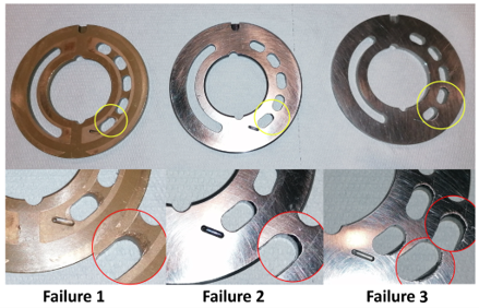
Each row in the dataset represents a single observation from an experimental run. It includes real-time measurements of eight distinct parameters and captures real-time measurements of critical performance indicators. 1. Pressure-leak line is the pressure at the location of fluid leakage. This line reflects internal resistance or pressure losses due to wear. 2. Temperature-leak line measures the thermal profile near the site of leakage. It is a measure of friction-induced heating. 3. Pressure-output measures how the system performs under load and is the fluid pressure from the pump  4. Temperature-suction line is the temperature at the intake and can tell us whether elevated inlet temperatures contribute to cavitation or inefficiency. 5. Temperature-output is the fluid temperature post-compression. This value represents energy transfer into the fluid and thermal load across the pump. 6. Flow-leak line is the volume of unintended fluid escaping per unit of time and a measure of internal degradation. 7. Flow-output is directly related to the overall performance and is the volume of fluid delivered by the pump. 8. Temperature difference is the difference between leak-line temperature and suction-line temperature. This indicates abnormal thermal behavior from mechanical wear or fluid anomalies. The study categorizes valve plate failures into three levels of cavitation damage which directly influence the pumps’ efficiency and reliability.  Minor cavitation damage is characterized by small pits and surface erosion which causes minimal impact on performance. Deeper erosion and material loss which results in efficiency reductions and minor leakage issues is considered moderate damage. The damage is considered severe with extensive material removal resulting in significant leakage and a drastic decline in performance. Figure 1 shows photographs of the three valve plate failure cases. Failure 2 represents the smallest damage state, Failure 1 a moderate damage state, and Failure 3 the largest damage state. These damage states were used to define the failure labels throughout the dataset. Machine learning models were trained and evaluated with the corresponding sensor measurements for each operating condition.

Two preprocessing steps were performed prior to the development of the machine learning models. First, any rows containing missing values were removed. The values were then averaged over one-second intervals to reduce data redunancy from high sampling frequency. There were a total of 146,359 usable observations after preprocessing. This included 68,347 healthy samples: 47,207 samples from Failure 1, 14,333 from Failure 2, and 16,472 from Failure 3.

Methodology

Input Features and Output Target

The output variable in Table 1 is 0 for normal operation and 1 for any degree of failure.  The three different examples of failure cases (Failures 1, 2, and 3) are collectively labeled as failure cases in the output classification.

The input consists of eight continuous sensor readings which describe the hydraulic power unit’s operational state. (Table 1) Deviations of thermal, pressure, and flow during pump operation can indicate potential failures.

	Variable Name	Variable Description
Input	Pleak line	pressure leak line
	Tleak line	temperature leak line
	Poutput	pressure output
	Tsuction line	temperature suction line
	Toutput	temperature output
	Fleak line	flow leak line
	Foutput	flow output
	Tdiff	Tleak line – Tsuction line
Output	binary label	normal or failure operating conditions

Data Preprocessing

Feature scaling was performed prior to training. The eight input features were standardized using StandardScaler for the feedforward Neural Network,. The scaler was fitted on the training data and then the transformation  applied to the validation and test sets. This ensured that the scaling parameters were estimated without information from the validation or test data. The remaining models used same preprocessing procedures described for their respective experiments.

We used a shift function to generate lagged features for the modes that treat observations independently. This was done by offsetting each value by a specified number of steps for all eight input variables in Table 1. New columns were created for each lag we chose.To ensure comparability, lag intervals from the study by Rojek and Blachnik¹ were replicated, followed by additional experiments using alternative lag values to assess their impact on model performance. Rojek and Blachnik¹ experimented with autoregressive features by including up to three historical samples (i.e., values from the previous three seconds). We hypothesize that the short lag windows Rojek and Blachnik may not capture the behavior associated with long-term and gradual cavitation-induced degradation.  We tested both short-term and long-term lag combinations on baseline models and during hyperparameter tuning. To clarify the terminology, “lag 1” refers to shifting a variable by 1 second into the past and “lag 60” refers to a 60-second shift, etc. We used comparisons of lag 0 to other lags as short as 1 second and as long as 60, 600 and 6000 seconds. Because the 6000-second lag was generated separately for each operating-condition dataset, the first 6000 observations in each dataset did not have a complete lag history and were excluded from that lagged-feature experiment. This left 62,347 healthy, 41,207 Failure 1, 8,333 Failure 2, and 10,472 Failure 3 observations. A range of lag values was evaluated because the optimal lookback is problem dependent and needs to be determined empirically¹⁰. After preprocessing removed rows with missing values, the healthy, Failure 1, Failure 2, and Failure 3 datasets contained 68,347, 47,207, 14,333, and 16,472 observations, respectively. Random Forest, XGBoost, and the feedforward Neural Network used these datasets and had identical sample counts. LSTM operates on fixed-length input sequences rather than on individual observations, so has different sample counts. Sequences were generated separately within each experimental run to ensure that no sequence crossed the boundary between healthy and failure experiments. With a sequence length of 600 and a stride of one, each sequence contains 600 consecutive observations followed by a label corresponding to the observation. Since each run must use the initial 600 observations to form the first sequence in LSTM, there are 600 fewer labeled LSTM samples compared to the observation-level dataset. This difference is reflected in Table 4.

Train-Validation-Test Split

The dataset was split into training, validation, and testing sets consistent with the procedure recommended and used by Rojek and Blachnik and ensures comparability with their results. Following their procedure, the final 15,000 healthy-condition samples were included in both the validation and test sets. This results in shared healthy-condition samples between these two sets, which may lead to optimistic estimates of generalization for the healthy class and is a limitation of the present work. Because the number of samples collected for Failure 1 was much higher than for the other sets, only Failure 1 data was used to represent failed conditions in the training set. The data corresponding to Failure 2 was used exclusively as a validation set. This allowed for tuning and model selection on failure conditions that were not observed during training. The data from Failure 3 was reserved entirely for the test set, providing new data for final performance evaluation. The use of three separate data sets allows the model to be trained and assessed on different cavitation-induced damage patterns.  The training set contains all samples used to learn model parameters, the validation set is used to tune hyperparameters, and the Failure 3 data was reserved for final performance evaluation.

All of the no-failure data except the last 15,000 samples, was used for training. The final 15,000 samples of no-failure data were then included in both validation and test sets. This ensured that the testing phase had a consistent reference for normal behavior across both validation and test cases. Table 2 shows the final sample counts in train, validation and test sets. The train-validation-test split allowed the model to learn from clear examples of working and faulty systems and then be validated and tested on new failure cases to evaluate its generalizability.

Target	Train Set	Validation Set	Test Set
Normal	53347	15000	15000
Failure	47207	14333	16472

Models and Evaluation Metrics

In non-sequential deep learning models, observations are treated independently and temporal structure is introduced only through engineered lagged features. They are used to provide a reference for performance from models using simplified assumptions about time. Sequential deep learning models explicitly incorporate events that happen over time since they are trained on ordered sensor measurements. Because these two categories of model handle information regarding time in two very different manners, an assessment of the effects of temporal information methods on predictive accuracy can be made.

Non-Sequential Models with Lagged Features

We evaluated four models: 1. Random Forest¹¹, 2. XGBoost¹², 3. a feedforward Neural Network¹³, and 4. a Long Short-Term Memory (LSTM) network¹⁴. Random Forest is versatile, robust to overfitting, and handles complex relationships well. However, it can be slow to train and challenging to interpret due to the large number of trees. XGBoost is highly accurate and efficient with large, complex datasets but needs to be tune carefully and requires a lot of computation. This makes it harder to train compared to simpler models. The Feedforward Neural Network is flexible and can detect non-linear relationships in data, particularly when multiple hidden layers are used. This is particularly true when multiple hidden layers are used¹³. It can automatically learn high-level feature representations and adapts well to large datasets. However, neural networks require careful tuning of numerous hyperparameters, are computationally intensive to train. They are often considered “black box” models as they are difficult to interpret. The Random Forest, XGBoost, and feedforward Neural Network models are non-sequential, meaning that each observation is independent. They do not inherently account for the order of data points. This can be problematic in time series contexts. In response, lagged features are constructed that inject past information into each data point, so some time-based patterns can be captured indirectly. Details on how these lagged features were constructed can be found in the data preprocessing section.

We looked at precision, recall, and the F1-score to assess model performance. Precision tells us how many of the predicted positives were correct.   Recall reflects how many positives were captured. The F1-score is a calculation that incorporates both precision and recall. In addition, we report the area under the receiver operating characteristic curve (ROC–AUC). The ROC-AUC evaluates the model’s ability to discriminate between normal and failure conditions. We also looked at performance on the training, validation and test sets to evaluate for generalizability across different scenarios and identify potential overfitting.

Grid searches were used to systematically test various hyperparameter combinations for both Random Forest and XGBoost classifiers to identify the most effective setup for model generalization and performance¹⁵. We used time series cross-validation with 10 splits in our validation process, similar to Rojek and Blachnik’s study¹. Training on earlier data and validating on later data prevents the mixing of past and future observations from confounding model training. We used the F1-weighted scoring metric which balances precision and recall. F1 score accounts for class imbalance by weighting scores according to class frequency.

Common and well-validated configurations in the literature were used to select the parameters and their values. As show in table 3, the hyperparameters of n_estimators, max_features, min_samples_split, and max_depth were tuned for the Random Forest Model. Multiple values for the n_estimators parameter were tested [100, 500, 1000] to see how the model performed with increasing complexity. This was done as increasing the number of trees is known to reduce variance and improve generalization up to a saturation point^11,16. Max_features, the number of features considered at each split, was varied from 1 to 8 (maximum number of features) to control the randomness and reduce correlation between trees. This increases ensemble diversity and robustness^11,17. Min_samples_split was tested from 20 to 200 in increments of 10. This sets the minimum number of samples needed to split an internal node and both limits overly deep trees and reduces overfitting¹⁸. Max_depth varied tree depth values from 2 to 20 in increments of 2 and also added a value for unrestricted depth to control the bias–variance tradeoff inherent in decision tree learning¹⁷.

Six hyperparameters in the XGBoost model were tuned to give the maximum flexibility and control over learning (Table 3). N_estimators was evaluated across the values of 100, 500, and 1000. Varying the number boosting iterations directly influences model capacity and overfitting behavior^19,12. The learning_rate, also known as eta, controls how quickly the model learns and was varied from 0.001 to 0.3. This compared conservative versus aggressive updates since lower learning rates are known to improve generalization at the cost of additional boosting rounds¹⁹. Max_depth was tested at values from 2 to 20 in increments of 2, as well as at unlimited depth, regulating tree complexity and preventing overfitting in gradient-boosted modelsmodels^12,18. We also adjusted subsample, the fraction of training instances used per tree, across values from 0.5 to 1.0 in increments of 0.1 to introduce introduces stochasticity in order to reduce variance and improve robustness¹⁹. Colsample_bytree determines the fraction of features used per tree and was varied from 0.5 to 1.0 in increments of 0.1 to encourage feature diversity and mitigate the dominance of highly correlated inputs¹². Together, these parameters enabled flexibility to balance model performance and generalization.

Seven hyperparameters were tuned for the feedforward Neural Network model in order to optimize its architecture, learning dynamics, and regularization (Table 3). The number of hidden layers was varied from 1 to 5 in increments of 1. This allowed different levels of model depth and abstraction. Deeper architectures enable hierarchical feature learning at the cost of overfittingoverfitting¹³. The neuron number in each layer was varied [16, 32, 64, 128, 256]. This trades off representational capacity against overfitting risk^13,20. The learning rate was varied [0.0001, 0.001, 0.01]  to test both conservative and aggressive learning schedules by controlling the step size during optimization. Learning rate affects how well the model converges during training and can affect final model performanceperformance²¹. The batch size was varied [8, 16, 32, 64] to examine its effect on training stability and convergence. We also experimented with dropout rates of [0, 0.1, 0.2, 0.3, 0.5] by randomly deactivating neurons during training. Both smaller batch size and dropout can introduce gradient noise and improve generalization²². Batch normalization was either enabled or disabled to reduce internal covariate shift and increase learning rates by normalizing intermediate layer outputs²³.

Model	Parameter	Range
Random Forest	n_estimators	[100,500,1000]
	max_features	Between 1 and 8 with increment of 1
	min_samples_split	Between 20 and 200 with increment of 10
	max_depth	None, between 2 and 20 with increment of 2
Xgboost	n_estimators	[100,500,1000]
	learning_rate	Between 0.001 and 0.3
	max_depth	None, between 2 and 20 with increment of 2
	subsample	Between 0.5 and 1 with increment of 0.1
	colsample_bytree	Between 0.5 and 1 with increment of 0.1
Feedforward NN	number of layers	Between 1 and 5 with increment of 1
	number of neurons	[16, 32, 64, 128, 256]
	learning_rate	[0.0001, 0.001, 0.01]
	batch_size	[8, 16, 32, 64]
	dropout_rate	[0, 0.1, 0.2, 0.3, 0.5]
	batch_norm	[True, False]
LSTM	number of layers	[1, 2, 3, 4, 5]
	number of neurons	[16, 32, 64, 128, 256]
	learning_rate	[0.0001, 0.001, 0.01]
	dropout_rate	[0, 0.1, 0.2, 0.3]
	batch_size	[8, 16, 32, 64]
	sequence_length	[60, 300, 600]

Sequential Models

Long Short-Term Memory (LSTM) networks are a specialized type of Recurrent Neural Network (RNN) which capture both short-term and long-term dependencies to learn from sequential data¹⁴. Traditional RNNs are limited in their ability to learn from long sequences since they struggle with vanishing and exploding gradient problems. LSTMs address this with a unique cell structure that includes input, output, and forget gates. These gates regulate the flow of information through the network and allow it to selectively remember or forget information over time. The ability to regulate information and learn from long sequences makes LSTMs effective for time series applications such as predictive maintenance, anomaly detection, and fault diagnosis^7,8.

The raw sensor data was restructured into overlapping time windows so that the LSTMs would have the sequential inputs they required. Each sequence was a continuous segment of readings across all eight sensors for a fixed number of timesteps. A window length of 600 timesteps would capture 600 seconds of sensor data into each training instance.  The label immediately following the sequence denotes the pump’s operating condition (healthy or failure). Window length is an important tuning parameter. Short sequences are sensitive to transient fluctuations but can be too short to detect larger patterns present in that longer sequences. Longer sequences have more historical context but increase the amount of computation needed and can overfit the data.

For the LSTM model, hyperparameters for architectural depth, representational capacity, and temporal context were adjusted to explore their effects on fault detection, as shown in Table 3. For architectural depth, the number of recurrent layers was varied from 1 to 5 to see how deeper hierarchies affect feature extraction¹⁴. For representational capacity, the number of hidden units within each LSTM layer was adjusted [16, 32, 64, 128, 256] to study its influence on both learning stability and generalization^24,13. Since dropout has been shown to improve generalization in recurrent neural networks, different dropout rates [0, 0.1, 0.2, 0.3] were applied to each recurrent layer. Dropout can mitigate overfitting at the expense of information retention²⁵. The final output layer used a single sigmoid-activated Dense neuron to classify each sample as either cavitation or non-cavitation. Training-related hyperparameters were tuned. Varied batch sizes were tried [8, 16, 32, 64] to see they had any effect on gradient stability or how quickly the  model learned²². Sequence length was varied [60, 300, and 600 timesteps] to see if temporal context length had an effects²⁶. These sequence lengths represent short-, medium-, and longer-duration contexts and were chosen to study the effect of increasing historical information on classification performance. Input sequences were generated separately within each experimental run after dataset partitioning. Consecutive sequences were created using a sliding window with a stride of one sample; therefore, adjacent 600-sample input windows overlap by 599 samples (99.83%). Sequence generation was restarted at every experimental-run boundary so that no sequence crossed between healthy and failure experiments or between the training, validation, and test datasets. The number of training epochs was constant at 50, and Adam optimizer was used for model training across all experiments. The learning rate for the feedforward Neural Network was also varied following the same range, [0.0001, 0.001, 0.01], to assess its impact on convergence behavior and generalization performance, as shown in table 3²⁷. We used a binary cross-entropy loss function for the fault-detection task. SHAP analysis (GradientExplainer from the SHAP library) was performed to improve the interpretability of the best-performing LSTM model. A background dataset consisting of 20 randomly selected training sequences was used as the reference dataset, and SHAP values were computed for a balanced sample of 100 test sequences (50 Normal and 50 Failure 3). SHAP values were computed for every timestep and feature within each sequence. For the per-sample plot, signed SHAP values were averaged across the 600 timesteps of each sequence. Global feature importance was calculated as the mean absolute SHAP value across all samples and timesteps for each sensor.

Similarly to non-sequential models, to assess sequential model performance, we rely on precision, recall, and F1-score, the area under the receiver operating characteristic curve (ROC–AUC). Given that the dataset is relatively well balanced, ROC–AUC provides a robust, threshold-independent measure of overall separability between classes. Similarly, we compare train performance with distinct validation and test sets to evaluate generalization over time.

Results and Discussion

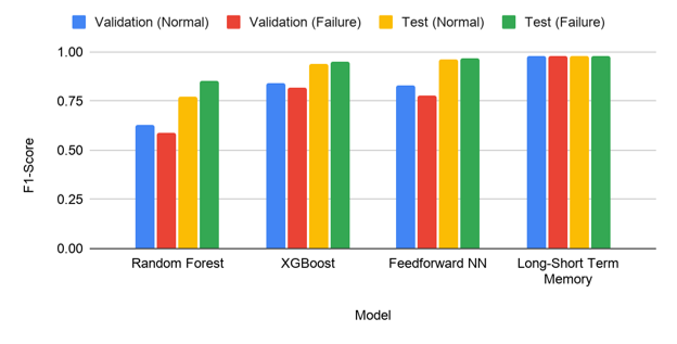
Here, we evaluate the machine learning models for their effectiveness in detecting cavitation-induced fault detection in hydraulic piston pumps. The predictive performance of non-sequential and sequential models is assessed using standard classification metrics. Model generalizability, performance differences between different approaches, and feature-level interpretability are then analyzed with SHAP. Finally, SHAP and standard classification are combined for quantitative and qualitative analysis of model effectiveness and practical relevance.Table 4 summarizes the precision, recall, F1-score, and ROC AUC results for all models across all datasets.  The Random Forest model shows perfect performance on the training set, with F1-scores of 1.00 for both Normal and Failure classes, followed by a substantial drop in validation performance to F1-scores of 0.63 (Normal) and 0.59 (Failure). This gap suggests overfitting to the training data and limited generalization to the validation condition. Test performance improves relative to validation, achieving F1-scores of 0.77 (Normal) and 0.85 (Failure), but still underperforms compared to other models. The XGBoost model demonstrates strong and consistent performance across datasets. Validation F1-scores reach 0.84 for Normal and 0.82 for Failure, while test F1-scores further improve to 0.94 and 0.95, respectively (Table 4, Figure 2). The higher scores for training compared to validation indicate some overfitting on the validation set. However, the overall the model shows robust generalization and effective learning of nonlinear feature interactions.

The scaled feedforward Neural Network achieved validation F1-scores of 0.83 for the Normal class and 0.74 for the Failure class. Performance improved on the Failure 3 test condition, with F1-scores of 0.94 for both Normal and Failure (Table 4, Figure 2), indicating stronger performance on the test condition than on the validation condition. The LSTM model achieved validation F1-scores of 0.90 for the Normal class and 0.88 for the Failure class. Performance increased on the Failure 3 test condition, with F1-scores of 0.97 for Normal and 0.98 for Failure (Table 4, Figure 2), demonstrating strong test-set classification performance while also indicating a noticeable difference between validation and test performance. The data shows that sequence modeling and learning temporal dependencies are effective for cavitation-related fault classification.

Figure 2 Compares validation and test F1-scores for the models. The Random Forest model underperforms other models during validation. XGBoost and the feedforward Neural Network show strong performance. The LSTM model had excellent F1-scores across all evaluation sets.

Model	Train/ Test	Label	Preci- sion	Recall	F1	ROC AUC	Samples
Random Forest   n_estimators = 100 max_features = 7 min_samples_split = 90	Train	Normal	1.00	1.00	1.00	1.00	53347
		Failure	1.00	1.00	1.00		47207
	Valid	Normal	0.61	0.64	0.63	0.55	15000
		Failure	0.60	0.57	0.59		14333
	Test	Normal	0.97	0.64	0.77	0.82	15000
		Failure	0.75	0.98	0.85		16472
Xgboost   n_estimators = 200 learning_rate = 0.3 max_depth = 4 subsample= 0.9 colsample_bytree = 0.9	Train	Normal	1.00	1.00	1.00	1.00	53347
		Failure	1.00	1.00	1.00		47207
	Valid	Normal	0.80	0.88	0.84	0.89	15000
		Failure	0.86	0.77	0.82		14333
	Test	Normal	1.00	0.88	0.94	0.98	15000
		Failure	0.90	1.00	0.95		16472
Feedforward NN   Layers: 4 Neurons per Layer: 128 Learning Rate: 0.01 Batch Size: 64 Dropout Rate: 0.5 Batch Normalization: False Feature Scaling: Standard Scaler	Train	Normal	0.89	0.99	0.94	0.98	53347
		Failure	0.99	0.86	0.92		47207
	Valid	Normal	0.72	0.98	0.83	0.68	15000
		Failure	0.97	0.60	0.74		14333
	Test	Normal	0.90	0.98	0.94	0.98	15000
		Failure	0.98	0.90	0.94		16472
Long-Short Term Memory   sequence_length = 600 batch_size = 64 num_layers = 2 units = 128 dropout = 0.3 epochs = 50	Train	Normal	1.00	1.00	1.00	1.00	52747
		Failure	1.00	1.00	1.00		46607
	Valid	Normal	0.85	0.95	0.90	0.98	14400
		Failure	0.95	0.83	0.88		13733
	Test	Normal	1.00	0.95	0.97	0.99	14400
		Failure	0.96	1.00	0.98		15872

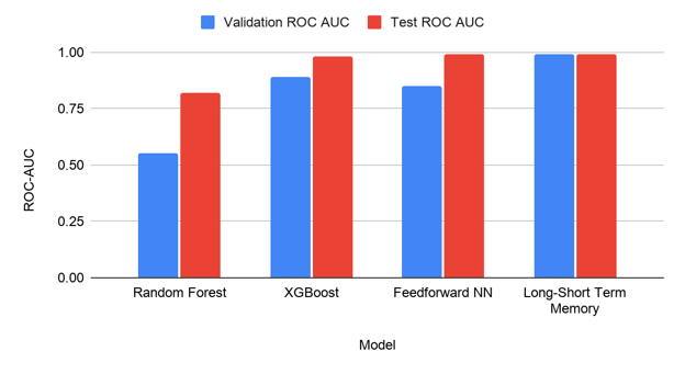
As shown in Table 4 and Figure 3, the Random Forest model achieves a validation ROC AUC of only 0.55, indicating weak separation between Normal and Failure classes, though its test ROC AUC improves to 0.82. XGBoost demonstrates strong discrimination, with ROC AUC values of 0.89 on validation and 0.98 on the test set as shown in Table 4 and Figure 3. The scaled feedforward Neural Network exhibits a larger difference between evaluation conditions, achieving a ROC–AUC of 0.68 on the validation set and 0.98 on the test set. The LSTM model demonstrates strong discriminative performance, achieving ROC–AUC values of 0.98 on the validation set and 0.99 on the test set (Table 4, Figure 3).

All reported classification metrics were obtained using the default decision threshold of 0.5. An optimal decision threshold would depend on operational requirements and whether false positives or false negatives carry greater costs. A lower threshold increases sensitivity to failures at the expense of more false positives, whereas a higher threshold can reduce unnecessary maintenance actions but at the risk of missing failures. Operational priorities of the intended deployment environment should consequently inform selection of the decision threshhold. Optimizing this threshhold for specific industrial applications could be the subject of future work.

Comparing training and validation/test results for each model shows important differences in generalizability. Both the Random Forest and XGBoost models performed perfectly during training, but the Random Forest model did poorly on the validation set. The likely explanation for this is overfitting. XGBoost performed strongly on validation and had a smaller gap between training and validation as a result. The feedforward Neural Network also showed a substantial training-to-validation performance gap for the Failure class, indicating weaker generalization to the Failure 2 validation condition. Similar to Random Forest and XG Boost, LSTM achieved perfect training performance but lower validation performance, also indicating some overfitting. Validation performance remained strong, suggesting that it generalized well to the unseen Failure 3 condition.

Performance on the test set is consistently higher than on the validation set for non-sequential models. This suggests that the Failure 3 test condition is more readily distinguishable from normal operation than the Failure 2 validation condition. Because only one failure run was available for validation and one for testing, it is indeterminate whether this is related to intrinsic characteristics of the Failure 2 and Failure 3 cases or broader differences in cavitation severity. Additional experiments using a large number of independent failure runs would be needed to make this assessment.

We tuned all models and evaluated their predictive performance on the validation and test sets. Then, we conducted pairwise McNemar tests to see if the differences in classification accuracy was statistically significant. The McNemar test analyzes disagreement patterns to compare classifiers on the same dataset and distinguishes whether differences are due to chance or meaningful performance advantage.

For the McNemar analysis, one LSTM window was selected every 600 samples separately within each test experimental run. This was done because treating every LSTM prediction as a separate comparison would have created dependence between adjacent units from the significant overlap between stride-one LTSM windows. There were 51 aligned non-overlapping comparison units in all (24 healthy and 27 Failure 3).  So models were compared on the same units, predictions from the Random Forest, XGBoost, and feedforward Neural Network were evaluated at the corresponding target observations. Exact two-sided McNemar tests were performed for all six pairwise model comparisons, with Holm correction applied to account for multiple comparisons.

The results in Table 5 show that, after Holm correction, only the comparison between Random Forest and XGBoost was statistically significant (adjusted p = 0.023). There was no statistical significance in the remaining five pairwise comparisons. Though the LSTM achieved the highest aggregate test performance, the McNemar analysis on the 51 non-overlapping comparison units does not show statistically significant differences between the LSTM and the other models.

Model A	Model B	A+/B-	A-/B+	Raw p-value	Holm-adjusted p-value	Significant
Random Forest	XGBoost	0	9	0.004	0.023	Yes
Random Forest	Feedforward NN	3	11	0.057	0.229	No
Random Forest	LSTM	2	11	0.022	0.112	No
XGBoost	Feedforward NN	3	2	1.0000	1.0000	No
XGBoost	LSTM	2	2	1.000	1.0000	No
Feedforward NN	LSTM	2	3	1.0000	1.0000	No

Based on the aggregate validation and test metrics, the LSTM was selected for SHAP analysis. SHAP(SHapley Additive exPlanations) helped to attribute each LSTM model prediction to individual input features, allowing both local (per-sample) and global (dataset-level) interpretation of model behavior. By evaluating both per-sample and aggregate contributions, SHAP analysis allows us to understand which sensor signals help to predict different failure scenarios and to identify consistent indicators of cavitation-induced degradation.

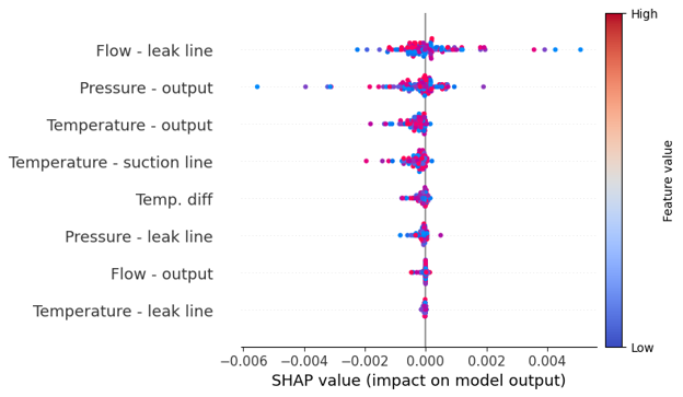
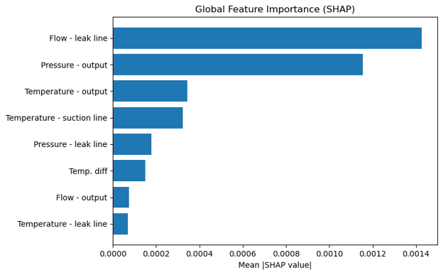
The top plot (per-sample SHAP) in Figure 4 shows how individual features influence each prediction across the dataset. The SHAP analysis identified leak-line flow as the most influential feature, followed by output pressure, temperature-output, and suction-line temperature. Rojek and Blachnik¹ also found leak-line flow and output pressure to be among the most important variables. However, our LSTM-based SHAP analysis assigns relatively greater importance to temperature-output than the baseline study, suggesting that temporal modeling may capture additional information contained in the evolution of thermal measurements. The bottom plot (global mean SHAP) shows that, overall, leak-line flow is the most important feature, followed by output pressure, temperature-output, and suction-line temperature. The order of importance assigned by SHAP agrees with our empiric understanding of hydraulic systems and the results of prior studies. Increases in leak-line flow and pressure are related to earlier findings of internal wear and cavitation damage, while reductions in output pressure and flow are related to subsequent declining pump performance. These insights from the model are of practical use, as operators can focus on the most informative measurements for fault detection, condition monitoring, and maintenance planning. The SHAP analysis helps to explain which sensor inputs influenced the LSTM predictions and are therefore most relevant to hydraulic system operation. The relative differences between features is more important than the absolute magnitudes, since SHAP values are aggregated along long sequences. The slight ordering differences among lower-ranked features arises from their different aggregation procedures. The per-sample plot uses signed SHAP values averaged across timesteps while the global plot uses mean absolute SHAP values across all samples and timesteps.

A key finding of this study is the noticeable performance gap between sequential and non-sequential models. Using lagged-feature partially captures temporal context, but may not fully capture the long-term dependencies associated with gradual cavitation damage. The LSTM explicitly learns across extended time horizons and better captures patterns associated with cavitation damage. This is shown in the higher F1-scores and ROC–AUC values on both validation and unseen failure test sets.

Our results outperform previously reported models for hydraulic pump fault detection. Using static machine learning models, Rojek and Blanchnik reported classification accurances below 90%. On the failure 1 dataset, they reported accuracies of 0.8455 for Gradient Boosted Trees, 0.8442 for Random Forest, and 0.8868 for the Multilayer Perceptron (MLP) model under optimal lag configurations. For unseen fault conditions, the MLP model achieved 0.8748 accuracy on Failure 2 and 0.8927 on Failure 3. Performance was moderately generalizable, but still below 90% in all cases. The LSTM performed better in aggregate on both validation and test conditions in this dataset than the previously reported models. These results suggest that sequence-based learning is beneficial for high-frequency sensor data in hydraulic systems.

The SHAP analysis shows that the model prioritizes sensor measurements associated with hydraulic pump condition. In particular, the prominence of leak-line flow and output pressure is broadly consistent with prior hydraulic fault studies^2,7,5,6. The agreement between the SHAP results and our prior physical understanding makes the LSTM results easier to interpret.

Knowing which measurements are most important for detecting failures allows engineers to optimize sensor placement during pump design and reduce costs which would be associated with placing additional sensors. It also allows them to focus on the most informative signals. Moreover, predictions from the models allow for planned and justifiable maintenance interventions based on interpretable evidence rather than opaque model output data.

Limitations

This study has several limitations. First, the experimental dataset is from a single hydraulic power unit and may not apply to other pump designs, or in other operating conditions or industrial environments. Different loads, temperatures, and other factors can all affect hydraulic systems, so the model might not apply to real-world conditions without additional retraining or adaptation even in pumps of similar design. Testing it in different conditions and on different machines would be needed.

Second, the number of measurements is limited to eight sensor readings. Other factors like vibration, acoustic emissions, and oil quality could help predict pump failures in addition to the pressure, temperature, and flow characteristics studied.

Third, the number of distinct failure modes is limited to three cavitation severity levels. Because LSTMs rely less on manually engineered input features, they may detect other hydraulic faults such as bearing wear or seal degradation. This would increase the utility of the model while still using the same measurement data.

Fourth, we adopted the same train-validation-test partitioning strategy as Rojek and Blachnik¹, so that our study could be directly compared with their experimental protocol. As a result, although the failure cases are different, the validation and test sets share the same healthy-condition samples. While this allows for a direct comparison with the baseline study, the shared controls may result in optimistic estimates of the healthy class performance. Evaluating the proposed models using fully independent validation and test sets should be a future research goal. This would assess model generalizability in a more rigorous manner.

Fifth, the validation and test datasets have a single independent failure run. The differences in model performance between these datasets suggest that some failure cases may be easier to classify than others. A larger collection of different pump failure scenarios is needed for additional validation.

Finally, each deep learning model was trained and evaluated using a single random initialization and data partition. Though this is consistent with the baseline study used for comparison, it nonetheless represents a single experimental outcome.

Conclusions

This study set out to develop and evaluate machine learning approaches for fault detection of cavitation-induced valve plate failures in hydraulic piston pumps using sensor data. We show that explicitly modeling temporal dependencies can improve predictive performance.

LSTM performed best overall, with the highest aggregate F1-score and ROC–AUC on both validation and test datasets. These results were numerically better than those reported in previous work. However, after correcting for multiple comparisons, pairwise McNemar testing on non-overlapping comparison units did not show statistically significant differences between the LSTM and the other models.

Beyond performance, SHAP analysis showed that the LSTM predictions were influenced most strongly by leak-line flow, output pressure, and temperature-output. These results provide insight into the sensor measurements most strongly influencing the model’s predictions.

While the study is limited by the scope of the dataset and feature availability, the results demonstrate the value of sequence-based learning and explainable AI for hydraulic system diagnostics.

References

1. Rojek, Marcin, and Marcin Blachnik. “A Dataset and a Comparison of Classification Methods for Valve Plate Fault Prediction of Piston Pump.” Applied Sciences, vol. 14, no. 16, Aug. 2024, p. 7183. DOI.org (Crossref), https://doi.org/10.3390/app14167183. [↩] [↩] [↩] [↩] [↩] [↩] [↩] [↩] [↩] [↩] [↩] [↩]
2. Xia, Shiqi, et al. “Modelling and Fault Detection for Specific Cavitation Damage Based on the Discharge Pressure of Axial Piston Pumps.” Mathematics, vol. 10, no. 14, July 2022, p. 2461. DOI.org (Crossref), https://doi.org/10.3390/math10142461. [↩] [↩]
3. Neupane, Dhiraj, et al. “Data-Driven Machinery Fault Diagnosis: A Comprehensive Review.” Neurocomputing, vol. 627, Apr. 2025, p. 129588. ScienceDirect, https://doi.org/10.1016/j.neucom.2025.129588. [↩]
4. Yahya, Mohammed A., et al. “Deep Learning for Multivariate Time Series Anomaly Detection: An Evaluation of Reconstruction-Based Methods.” Artificial Intelligence Review, vol. 58, no. 12, Oct. 2025, p. 400. DOI.org (Crossref), https://doi.org/10.1007/s10462-025-11401-9. [↩]
5. Jardine, Andrew K.S., et al. “A Review on Machinery Diagnostics and Prognostics Implementing Condition-Based Maintenance.” Mechanical Systems and Signal Processing, vol. 20, no. 7, Oct. 2006, pp. 1483–510. DOI.org (Crossref), https://doi.org/10.1016/j.ymssp.2005.09.012. [↩] [↩]
6. Qi, Ruosen, et al. “A Review on Data-Driven Condition Monitoring of Industrial Equipment.” Algorithms, vol. 16, no. 1, Dec. 2022, p. 9. DOI.org (Crossref), https://doi.org/10.3390/a16010009. [↩] [↩]
7. Dai, Juying, et al. “Signal-Based Intelligent Hydraulic Fault Diagnosis Methods: Review and Prospects.” Chinese Journal of Mechanical Engineering, vol. 32, no. 1, Sept. 2019, p. 75. Springer Link, https://doi.org/10.1186/s10033-019-0388-9. [↩] [↩] [↩] [↩]
8. Xu, Yang, et al. “A Hybrid Deep-Learning Model for Fault Diagnosis of Rolling Bearings.” Measurement, vol. 169, Feb. 2021, p. 108502. DOI.org (Crossref), https://doi.org/10.1016/j.measurement.2020.108502. [↩] [↩] [↩]
9. Wu, Chunming, and Shupeng Zheng. “Fault Diagnosis Method of Rolling Bearing Based on MSCNN-LSTM.” Computers, Materials & Continua, vol. 79, no. 3, 2024, pp. 4395–411. DOI.org (Crossref), https://doi.org/10.32604/cmc.2024.049665. [↩] [↩]
10. Leites, José, et al. “Lag Selection for Univariate Time Series Forecasting Using Deep Learning: An Empirical Study.” arXiv:2405.11237, arXiv, 18 May 2024. arXiv.org, https://doi.org/10.48550/arXiv.2405.11237. [↩]
11. Breiman, Leo. “Random Forests.” Machine Learning, vol. 45, no. 1, Oct. 2001, pp. 5–32. DOI.org (Crossref), https://doi.org/10.1023/A:1010933404324. [↩] [↩] [↩]
12. Chen, Tianqi, and Carlos Guestrin. “XGBoost: A Scalable Tree Boosting System.” Proceedings of the 22nd ACM SIGKDD International Conference on Knowledge Discovery and Data Mining [San Francisco California USA], 2016, pp. 785–94. DOI.org (Crossref), https://doi.org/10.1145/2939672.2939785. [↩] [↩] [↩] [↩]
13. Goodfellow, Ian, Yoshua Bengio, and Aaron Courville. Deep Learning. MIT Press, 2016. [↩] [↩] [↩] [↩] [↩]
14. Hochreiter, Sepp, and Jürgen Schmidhuber. “Long Short-Term Memory.” Neural Computation, vol. 9, no. 8, Nov. 1997, pp. 1735–80. DOI.org (Crossref), https://doi.org/10.1162/neco.1997.9.8.1735. [↩] [↩] [↩]
15. Bergstra, James, and Yoshua Bengio. “Random Search for Hyper-Parameter Optimization.” Journal of Machine Learning Research, vol. 13, 2012, pp. 281–305. [↩]
16. Oshiro, Thais Mayumi, et al. “How Many Trees in a Random Forest?” Machine Learning and Data Mining in Pattern Recognition, edited by Petra Perner, Springer, 2012, pp. 154–68. Springer Link, https://doi.org/10.1007/978-3-642-31537-4_13. [↩]
17. Hastie, Trevor, et al. The Elements of Statistical Learning. Springer, 2009. Springer Series in Statistics. DOI.org (Crossref), https://doi.org/10.1007/978-0-387-84858-7. [↩] [↩]
18. Probst, Philipp, et al. “Tunability: Importance of Hyperparameters of Machine Learning Algorithms.” arXiv:1802.09596, arXiv, 22 Oct. 2018. arXiv.org, https://doi.org/10.48550/arXiv.1802.09596. [↩] [↩]
19. Friedman, Jerome H. “Greedy Function Approximation: A Gradient Boosting Machine.” The Annals of Statistics, vol. 29, no. 5, Oct. 2001. DOI.org (Crossref), https://doi.org/10.1214/aos/1013203451. [↩] [↩] [↩]
20. Srivastava, Nitish, Geoffrey Hinton, Alex Krizhevsky, Ilya Sutskever, and Ruslan Salakhutdinov. “Dropout: A Simple Way to Prevent Neural Networks from Overfitting.” Journal of Machine Learning Research, vol. 15, 2014, pp. 1929–58. [↩]
21. Bengio, Yoshua. “Practical Recommendations for Gradient-Based Training of Deep Architectures.” arXiv:1206.5533, arXiv, 16 Sept. 2012. arXiv.org, https://doi.org/10.48550/arXiv.1206.5533. [↩]
22. Keskar, Nitish Shirish, et al. “On Large-Batch Training for Deep Learning: Generalization Gap and Sharp Minima.” arXiv:1609.04836, arXiv, 9 Feb. 2017. arXiv.org, https://doi.org/10.48550/arXiv.1609.04836. [↩] [↩]
23. Ioffe, Sergey, and Christian Szegedy. “Batch Normalization: Accelerating Deep Network Training by Reducing Internal Covariate Shift.” arXiv:1502.03167, arXiv, 2 Mar. 2015. arXiv.org, https://doi.org/10.48550/arXiv.1502.03167. [↩]
24. Greff, Klaus, et al. “LSTM: A Search Space Odyssey.” arXiv:1503.04069, arXiv, 4 Oct. 2017. arXiv.org, https://doi.org/10.48550/arXiv.1503.04069. [↩]
25. Zaremba, Wojciech, et al. “Recurrent Neural Network Regularization.” arXiv:1409.2329, arXiv, 19 Feb. 2015. arXiv.org, https://doi.org/10.48550/arXiv.1409.2329. [↩]
26. Bengio, Yoshua. “Representation Learning: A Review and New Perspectives.” arXiv:1206.5538, arXiv, 23 Apr. 2014. arXiv.org, https://doi.org/10.48550/arXiv.1206.5538. [↩]
27. Kingma, Diederik P., and Jimmy Ba. “Adam: A Method for Stochastic Optimization.” arXiv:1412.6980, arXiv, 30 Jan. 2017. arXiv.org, https://doi.org/10.48550/arXiv.1412.6980. [↩]