Stability Analysis of Low-Earth-Orbit Mega-Constellations Under Debris Growth Using Probabilistic and Dynamical Systems Models

Abstract

Rapid deployment of mega-constellations into Low-Earth Orbit (LEO) has created a risk of collision cascade that existing regulatory and engineering frameworks are not built to handle. Kessler syndrome, a self-sustaining debris cascade capable of rendering entire orbital shells inaccessible, is shifting from theoretical possibility to operational concern. This paper develops and cross-validates a four-framework analytical model to determine the combination of satellite areal density and debris generation per catastrophic collision at which LEO debris growth becomes unstable. The frameworks are a discrete-state Markov chain of satellite lifecycle transitions, a coupled ordinary differential equation system for population-level satellite and debris dynamics, a 10,000-trial-per-parameter Monte Carlo simulation, and a graph-theoretic spectral analysis of the collision network. All four share a common mean-field description of a single orbital shell, so their agreement is an internal consistency check rather than four independent confirmations. All four locate the same instability threshold, expressed through a dimensionless collision reproduction number R₀=αβρₛ/δ; the threshold R₀=1 corresponds to a satellite population of order 10⁴ under canonical 550 km LEO parameters. In practical terms, the stable regime extends to roughly 20,000 satellites, a marginal zone occupies 20,000 to 38,000 satellites, and the system becomes dynamically unstable above approximately 38,000 satellites without aggressive debris mitigation. While many existing models are more detailed, they are computationally expensive and analytically opaque, which makes the location of the threshold hard to interrogate directly. These findings are therefore directly usable by constellation designers, debris-removal developers, and the regulators responsible for orbital-traffic policy.

Keywords: Kessler Syndrome, LEO mega-constellations, orbital stability, space debris, Markov chain, Monte Carlo simulations, dynamical system, graph theory, satellite density, active debris removal, space traffic management

Introduction

Spaceflight has a vast and extensive history, but in the last decade, particularly the last seven years, Low-Earth Orbit (LEO) has undergone a rapid and consequential transformation in space activity. For a majority of nearly seven decades after the launch of Sputnik in 1957, governmental agencies occupied the orbital environment by conducting carefully planned missions with one or two satellites at a time. That era of limited and careful engineering of satellites is now being transformed and heavily populated by private commercial operators who are pursuing high-speed internet connection on an industrial scale. The most prominent among these is SpaceX’s Starlink program, which received authorization for up to 42,000 satellites that were deployed in batches of 60 aboard reusable Falcon 9 rockets. The initiation of the Starlink program proved to be highly influential, accounting for roughly 70 percent of all operational satellites launched into orbit between 2019, when Starlink operations began, and early 2023, with the constellation continuing to expand since¹. Beyond Starlink, Amazon’s Project Kuiper has secured licenses for 3,236 satellites, the United Kingdom’s OneWeb has filed for over 6,000, and China’s state-backed Guowang constellation could eventually encompass an additional 13,000 objects². International projects such as the European Union’s IRIS² program add further to this growth, which recent projections suggest could bring the number of active LEO satellites to the order of 100,000 within the next two decades³.

This transformation in Low Earth Orbit offers indisputable social benefits. These mega constellations provide internet connectivity that has shown great potential in bridging the digital divide and supporting global real-time disaster response. Specifically, the LEO constellations offer latencies between 20 and 40 milliseconds as opposed to the 600-millisecond round-trip delays which are inherent to geostationary links (GEO links). LEO satellite signals also support Doppler-based positioning systems which calculate location based on shifts in signals between transmitters and their corresponding receivers, accurately locating other satellites within a 200-meter radius⁴. LEO constellation architecture can also provide early warning systems from space with a spatial coverage that exceeds any ground-based counterparts⁵. Their lower altitude provides for higher-resolution sensing and fast revisit times, which allows the constellations to quickly detect fast-moving threats such as hypersonic aircraft. Furthermore, since these constellations consist of coordinating satellites, they can track targets more reliably and maintain resilience even if individual satellites fail. These advantages explain why commercial operators have been so enthusiastic about these mega-constellations, as well as the robustness of the systems in providing continuous global data services⁶.

While these expansions are beneficial in the short-term advancement of communication, the orbital environment is still a finite space with a limited capacity for growth. Objects in LEO travel at a rate of 7.5 km/s, and the relative velocity between two objects intersecting orbital paths can range from 10 km/s to over 15 km/s. In addition, since mega-constellations occupy varying altitude bands, with the satellites within these bands sharing similar velocities, collision is sensitive to areal density, which is the number of objects per square meter of orbital surface area.  These speeds transform and scale the kinetic energy of objects in orbit drastically, where even a 1-centimeter aluminum sphere can have the kinetic energy equivalent to a hand grenade. Thus, a single collision could disperse on the order of 1,000 to 10,000 fragments spanning all size classes, of which typically several hundred are large enough (greater than roughly 10 cm) to be individually capable of triggering a further catastrophic breakup, and which persist as collision hazards for years to decades⁷. As of 2025, surveillance networks regularly track more than 35,000 objects larger than 10 cm, while statistical models maintained by the European Space Agency estimate on the order of one million objects between 1 and 10 cm and more than 100 million fragments smaller than 1 cm in Earth orbit^8,9. Thus, every new satellite added to the orbital environment increases collision probability, and since many objects are too small for routine tracking, satellites cannot maneuver to avoid these collisions^7,10.

The framework for understanding when this system might become self-reinforcing was established in a 1978 paper, where NASA scientist Donald J. Kessler and his colleague Burton Cour-Palais analytically demonstrated that at a certain orbital critical point, the rate at which collision-generated debris accumulates would exceed the rate at which debris is removed due to atmospheric drag, which would cause the orbital environment to enter a loop of self-sustaining cascades of satellite collisions¹¹. This theoretical framework, universally coined the Kessler Syndrome, has been studied and analyzed through increasingly sophisticated models. Hudson (2022) built KESSYM, a stochastic simulation finding that the Kessler Syndrome is statistically near inevitable within 200 to 250 years under baseline assumptions, although preventable with timely action¹². Sturza and Saura Carretero (2021) modelled the expected time to Kessler Syndrome as a function of satellite number, satellite size, and orbital configuration, and identified a safe-space boundary within that parameter space¹⁰. In accordance with this, debris removal measures have also drastically grown. To name a few, the European Space Agency (ESA)’s e.Deorbit program pioneered chaser-satellite architecture using robotic arms to capture tumbling objects such as ENVISAT, contactless plasma beam methods have demonstrated deceleration of debris without physical contact, and electromagnetic active debris removal (ADR) architectures promise cost reductions of 90 to 95 percent over conventional chemical-propulsion removal^13,14,8.

This threat is not only hypothetical but grounded in reality today. In 2009, the collision between the Iridium 33 satellite and the Russian Cosmos 2251 spacecraft created a significant threat to the orbital field at an altitude of 790 km, where more than 2,000 trackable fragments formed a debris cloud that is still in orbit today¹⁵. Furthermore, in 2019, the ESA was forced to execute a collision avoidance maneuver on their Aeolus Earth observation satellite to avoid hitting a Starlink satellite. This near collision highlights another structural asymmetry that was quantified by Bennett and Cudney (2026). Starlink accounts for 52 percent of all mass in LEO and 75 percent of all mass launched into LEO between 2019 and early 2023, which makes orbital sustainability and mega-constellation policy intrinsically linked¹.

The debris modeling community has responded with increasingly sophisticated tools such as NASA’s LEGEND, ESA’s MASTER, and MIT ARCLab’s MOCAT-MC toolbox. The findings obtained through the use of these tools have been substantial. For example, by utilizing MOCAT-MC, Appel’s 2024 master thesis at MIT found exponential growth in object populations as the LEO altitude increased, as well as an exceedance of the critical tipping point under baseline launch traffic¹⁶. However, while these tools provide a detailed simulation that can track thousands of fragments over a long period of time, many of them are computationally demanding. It would be inaccurate, however, to describe these tools as uniformly unavailable: ESA’s MASTER debris model can be obtained without charge through the Space Debris User Portal, and MIT ARCLab’s MOCAT-MC framework is released as open-source software. The more fundamental limitation is one of analytical transparency rather than access. As a result, these models create a barrier between the researchers who are noting these threats and the engineers and companies that need to act on them. These models are also limited because they provide numerical values, but not a real insight into the underlying structural causes of the instability¹⁶. While the numerical values are exact, the real structural instability drivers that shape how the system behaves, such as orbital interactions, density thresholds, and coordination effects, aren’t explained.

This paper will address this gap by developing a collection of simplified mathematical models that will identify the tipping point where LEO mega-constellations transition from a stable and sustainable operation, to one that is unstable and Kessler-like. The specific question being addressed is: at what combination of satellite areal density and debris-generation rate does the LEO debris system transition from stable to dynamically unstable behavior? To answer this question, four supporting frameworks will be utilized: a discrete Markov Chain model to capture the individual satellite lifecycle transitions; a system of coupled differential equations to govern satellite population and debris dynamics; Monte-Carlo simulations to validate the analytical thresholds under realistic assumptions; and a graph-theoretic collision-network analysis that captures how the satellites’ positions and movement patterns create connections, capturing both where they are in space and how they interact. The combination of these four frameworks on a single condition will establish a strong and transparent conclusion that can help policy makers to influence design guidelines and regulatory debris policies.

Background and Prior Work

The Physical Environment of Low-Earth Orbit

Conventionally, LEO spans 200 to 2,000 km above Earth’s surface, and it is the most dynamically active band where mega-constellations operate, and where debris accumulation poses the greatest long-term risk for near-Earth space. Satellites in this region orbit at velocities of approximately 7.5 km/s, completing a full circuit of Earth in roughly 90 to 120 minutes. Today, LEO hosts the large majority of all operational satellites, and a single commercial constellation accounts for over half of the total mass in that regime¹. High orbital velocity is beneficial for low-latency communications in LEO, but it also creates a major risk. Since the kinetic energy of a collision scales with the square of the relative velocity, even a minute impact can release energy comparable to several kilograms of high explosive for each kilogram of the object’s mass.

The classical collision rate model, which is identical to the molecular kinetic theory, gives the collision rate experienced by a given satellite as:

where ρ is the spatial number density of objects in the shell (per cubic meter), σ is the effective collision cross-section of the satellite (square meters), and v_rel is the mean relative velocity between objects in meters per second. This expression for collision rate is linear in terms of density and cross-sections, which means that the growth of the number of mega-constellations, as well as the trend for an increased cross-section for satellites, increases the collision rate simultaneously¹⁷. Furthermore, from the standpoint of navigation engineering, Tao et al. (2025) noted that growth of LEO communication satellites has reintroduced satellite selection challenges at an unprecedented scale, as each ground-based observer sees far more satellites than before¹⁸. Thus, this challenge provides more substantial evidence that accounting for density trajectory is vital in collision models.    

Two related densities appear in this paper and should be distinguished. The volumetric number density ρ (objects per m³) enters the classical collision rate above, whereas the population models below are written in terms of the areal density ρₛ(objects per m² of shell surface). For a shell of thickness H, the two are related by ρ=ρₛ/H, and it is this relation, with H≈50 km, that converts between the per-satellite collision rate and the shell-averaged quantities used later.

The orbital lifetime of debris in LEO varies dramatically with altitude. At 400 km, atmospheric drag is sufficient to deorbit most objects within months to a few years. At 550 km, orbital lifetimes extend to approximately five years for large objects, and considerably longer for smaller, denser debris fragments. Above 800 km, lifetimes can reach decades or centuries. For example, the 2007 Chinese ASAT test at 865 km altitude generated a debris cloud with long-lasting consequences for the orbital environment¹⁵. However, these debris clouds aren’t simply a collision hazard. Shareefdeen and Al-Najjar (2024) demonstrated that space debris has a full pollution cycle, from how fragments are created to when chemical byproducts are released as they burn in the atmosphere⁹. Furthermore, Mackintosh et al. (2026) highlighted that although most of this debris sits around a certain altitude, the peak collision probability is approximately 50 km above this debris-dense area³. The reason behind this, however, is intuitively straightforward. In efforts to avoid this debris dense area, satellites are located just above this altitude; however, to achieve the same high-quality resolution as it would be in the debris-dense area, the satellites must be bigger, and since there is an increased cross section for each satellite, the probability of collision is much higher.

The Kessler Syndrome: Formulation and History

The Kessler Syndrome was formally introduced by Donald J. Kessler and Burton G. Cour-Palais in their 1978 paper “Collision Frequency of Artificial Satellites: The Creation of a Debris Belt,” published in the Journal of Geophysical Research¹¹. Using straightforward kinetic theory, they established that the orbital environment had a carrying capacity that could be governed by the ratio of debris creation to debris removal rates. In essence, once the debris creation rate exceeds the rate at which debris is removed due to atmospheric drag, the system enters an unstable loop¹¹. The core condition for Kessler Syndrome is:

In the decades following Kessler and Cour-Palais’s work, the theory was refined by numerous researchers. Kessler himself refined the theory years later in 1991 and formalized the conditions for collisional cascading in terms of object population density thresholds (cited in Hudson, 2022)¹². In the years following this revisitation, the issue gained momentum as the hypothesized threats became reality. Specifically, the 2007 Chinese anti-satellite weapon test,  which destroyed the Fengyun-1C weather satellite, sent more than 3,000 cataloged fragments into a debris cloud, making it the most environmentally damaging fragmentation event on record¹⁵. This renewed urgency was further emphasized two years after, with the aforementioned 2009 Iridium-Cosmos collision and Hudson’s 2022 stochastic simulation KESSYM^9,12. In 2021, Sturza and Saura Carretero took an alternative approach, modelling growth of the object population with a nonlinear ordinary differential equation of the form:

The N² term of the ODE captures the essential quadratic growth of collision rate with object count, implying that doubling the satellite density roughly quadruples the pairwise collision rate. 

Active Debris Removal Technologies

The physical analysis of stability thresholds connects directly to the question of whether debris removal technologies can effectively shift those thresholds. ESA’s e.Deorbit program, detailed by Jaekel et al. (2018), created the chaser-satellite architecture, which consisted of a robotic arm capturing a tumbling object, stabilizing it, and then performing deorbit burn¹³. While this direct approach could be beneficial in the long run, many engineering challenges emerge from uncontrolled tumbling debris, and there are many ambiguities with obtaining objects that are outside of a country or state’s jurisdiction. However, contactless methods avoid the physical entanglement risks. Takahashi (2025) demonstrated a cusp-type bi-directional radiofrequency plasma thruster that uses a plasma beam to decelerate debris without causing any net force difference on the observer satellite itself¹⁴. Furthermore, Choueiri (2026) proposed electromagnetic debris removal systems, including orbital magnetic tugboats and momentum-exchange tethers, that predict per-object removal costs of roughly $300,000⁸. This is highly significant because it is roughly a 90 to 95 percent reduction compared to conventional chemical-propulsion approaches.  As these technologies are considered, they are reflected onto the debris decay rate parameter in the differential equation model of this paper, which raises the critical instability threshold.

Markov Chain and Monte Carlo Methods

The Markov chain framework that is highlighted later in this paper utilizes a well-established mathematical foundation. Using their Marathon Software library, Rechner and Berger (2016) showed that analyzing a single spectral measure of a state-transition graph gives a reliable estimate of how a Markov chain will settle into its long-term behavior¹⁹. These findings demonstrated that the single spectral measure closely predicted the chain’s mixing time, so it was useful to determine whether a satellite lifecycle will stabilize or remain unpredictable for a long period of time. Furthermore, the Monte Carlo simulation described later obtains collision events from a Poisson process and samples fragmentation counts from an empirical distribution²⁰. This process was executed using a randomized simulation approach, which has been validated in related debris-modeling studies such as Appel (2024) in the MOCAT-MC context and by Hudson (2022) in the KESSYM context^16,12.

Methods: A Multi-Framework Stability Analysis

The modeling approach that is developed here deliberately utilizes four distinct but complementary frameworks. As opposed to a single model of analysis, utilizing four different mathematical approaches, which rest on different mathematical assumptions but share a common mean-field description, provides an internal consistency check on the same critical threshold rather than four independent confirmations. These four frameworks, including a Markov chain analysis, coupled differential equation modeling, a Monte Carlo simulation, and a graph-theoretic analysis, are described in detail below.

Discrete-State Markov Chain Model

The first framework that will be utilized is the discrete-state Markov Chain Model. The model treats each individual satellite as its own system that transitions through the five operational states of a satellite. This approach captures the satellite lifecycle of each satellite irrespective of others, which allows for an analysis of how population behavior emerges and is altered by individual discrete-state transition probabilities.

The five operational states for the satellites are defined as follows: S₁ (Operational), where the satellite is functioning as it normally should; S₂ (Maneuvering), where the satellite is executing a maneuver in the effort to avoid collision; S₃ (Collision), where the satellite experiences a hypervelocity or catastrophic collision; S₄ (Debris), where the satellite has fragmented into debris; and S₅ (Deorbited), where the object has been removed from orbit, through natural atmospheric drag or a controlled deorbit. This framework uses finite Markov chains, where the fundamental matrix describes the expected lifecycle behavior of each satellite, as rigorously analyzed by Rechner and Berger (2016) for general state-graph analysis¹⁹. These transitions can be visualized more simply in Figure 1.

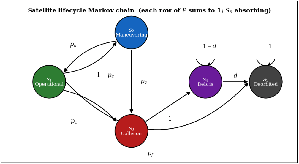
The transition matrix P governing evolution between states is:

rows sum to 1; state S₅ (Deorbited) is absorbing

where: p_c=ρ×σ×v_rel is the collision probability derived from the classical collision rate formula; pm is the probability of successful maneuver execution; pf is the satellite failure probability; and d is the debris decay rate, or the probability that a debris fragment deorbits due to atmospheric drag. All of these parameters are expressed as dimensionless probabilities that are scaled to a one-year time step in order to retain a consistent analysis.

The Markov chain has an absorbing state at S₅ (Deorbited), as well as a near-absorbing state at S₄ (Debris) if debris decay d is low (d≈0). One natural quantity to consider is the stationary distribution π = [π₁, π₂, π₃, π₄, π₅], which satisfies:

For an absorbing Markov chain, the stationary distribution places all probability on the absorbing (deorbited) state, so it cannot itself serve as a stability criterion. The chain is therefore analyzed through its fundamental matrix, which gives the expected time a satellite spends in each transient state, and hence its expected operational lifetime and its probability of suffering a catastrophic collision before it deorbits. With the corrected, row-stochastic transition matrix these quantities are well defined: for the nominal parameters the expected on-orbit lifetime is about five years, consistent with the five-year post-mission disposal rule, and the probability of a catastrophic collision during a satellite’s lifetime is on the order of one percent. These per-satellite statistics are conditional on a fixed background environment: the collision probability in the transition matrix is evaluated at the mean-field debris density of the shell, so the chain describes the life cycle of a representative satellite at a given ambient debris level rather than the coupled evolution of that level itself. Whether debris runs away at the population level is governed not by this single-satellite chain but by the reproduction number R₀ developed in the next framework.

Coupled Differential Equation Population Model

Contrary to the Markov chain model, which operates at the level of individual satellites, the differential equation framework describes the aggregate behavior of the satellite and debris populations as continuous dynamical systems. Let S(t) denote the total number of operational satellites and D(t) be the total number of debris fragments. The governing equations are:

In these equations, k=σvᵣₑₗ/V is the pairwise collision-rate coefficient (with the effective collision cross-section, vᵣₑₗ the mean relative velocity, and V=AₛH the volume of a shell of surface area Aₛ and thickness H); ρₛ is the satellite areal density (objects per m² of shell surface); is the natural satellite deorbit rate (per year); is the mean number of collision-capable fragments produced per catastrophic collision (of order 100, while the total number of fragments across all sizes is larger, roughly 1,000 – 10,000); and is the debris decay rate due to atmospheric drag (per year). The first equation states that the satellite population is replenished by launches at rate L and lost through natural deorbiting (rate μ) and collisions with debris (rate kSD). Operational satellites are assumed to actively avoid one another, so collisions between two functioning satellites are neglected; the dominant collisional risk, consistent with the 2009 Iridium–Cosmos collision, in which an active satellite struck a defunct one, is impact with untracked debris or defunct objects. The second equation states that debris is produced by collisions and removed by atmospheric decay (rate ). Crucially, the collision term includes both satellite-debris and debris-debris encounters (the SD and 1/2D² terms), so that existing debris can generate further debris. This pairwise structure follows the same kinetic-theory foundation from which the classical collision-rate formula was derived, and parallels the quadratic dependence of collision rate on object count in Sturza and Saura Carretero’s 2021 analysis¹⁰.

To understand how the debris population behaves over time, we examine the debris-free state, in which no fragments are present, and ask whether a small amount of debris introduced into the system will grow or decay. Using the debris growth equation established earlier:

Linearizing this expression about the debris-free state (S≈S₀ and D→0) and keeping the leading term in D gives:

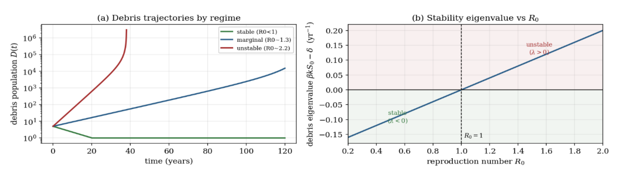
This shows that, near the debris-free state, a small amount of debris grows or decays exponentially at the rate βkS₀-δ. To determine stability, we therefore examine the sign of this rate, which is the relevant eigenvalue of the linearized system at the debris-free state.

The quantity βkS₀-δ is the key eigenvalue that tells us whether a tiny amount of debris will shrink or grow. If βkS₀-δ<0, the debris decays and the system returns to a clean-orbit state; if instead βkS₀-δ>0, the debris grows exponentially, even from the smallest of disturbances. Thus, setting βkS₀-δ=0 reduces the instability condition to:

Or if rearranged in terms of the critical density threshold:

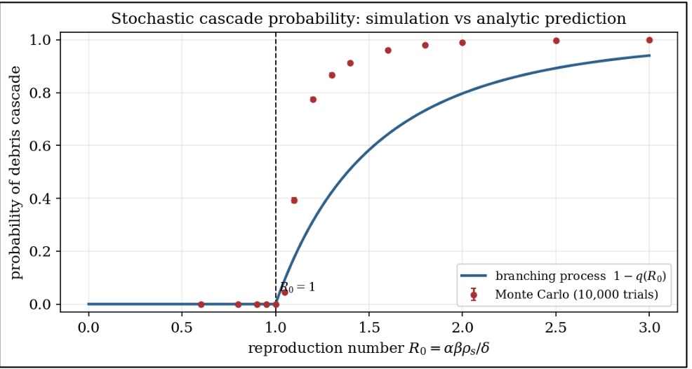
The reproduction number admits a direct probabilistic interpretation that links the deterministic threshold to the stochastic and network analyses that follow. R₀ can be read as the expected number of new catastrophic collisions produced, over its orbital lifetime, by the debris generated in a single collision: when R₀ is below one each collision replaces itself with fewer than one successor and any incipient cascade dies out, whereas when R₀ exceeds one collisions more than replace themselves and the debris population grows without bound. This is the same quantity that governs the branching process underlying the Monte Carlo simulation of the following section and the spectral radius of the collision network analyzed thereafter, so the transcritical bifurcation of the mean-field model, the runaway probability of the stochastic model, and the percolation threshold of the graph all refer to the single condition R₀ = 1.

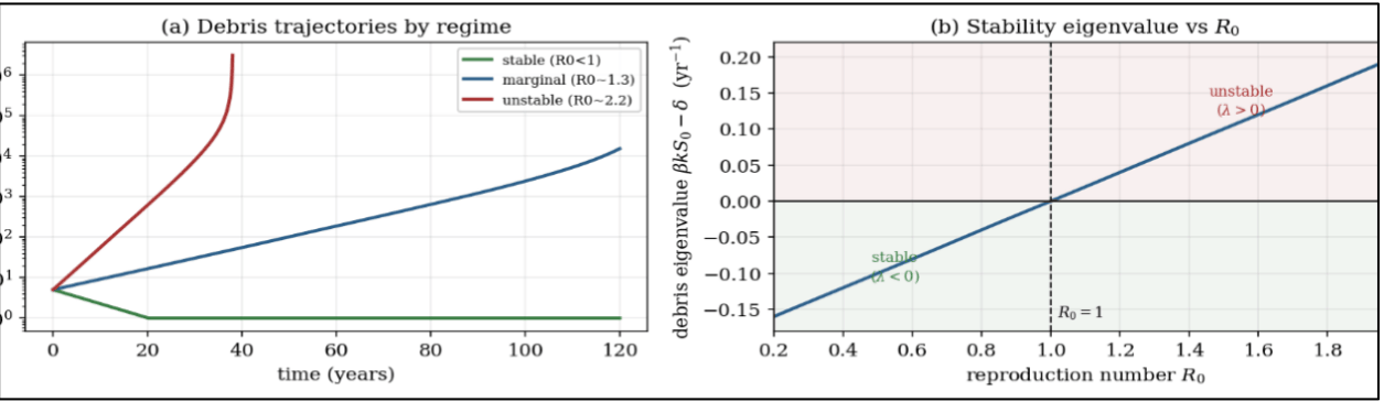
Once this condition is satisfied, small perturbations in the debris population cause unbounded growth rather than a return to equilibrium, which is the essential condition for debris instability. The advantage of this formulation is that it expresses the instability threshold as an explicit function of measurable parameters, which allows for the evaluation of any satellite/constellation scenario. This bifurcation-like behavior can be visualized more clearly in Figure 2.

Monte Carlo Stochastic Validation

The thresholds derived from the aforementioned models depend on simplifying assumptions, specifically the mean-field approximation that treats collision probability as a function of average density rather than a random variable. To assess the validity of these approximations under realistic randomness, a Monte Carlo stochastic simulation was implemented and executed for 10,000 independent trials per parameter configuration using easily accessible established frameworks, namely MATLAB and python.

In each trial, a population of N satellites was initialized within the orbital shell. At each time step, collision events were randomly sampled from a Poisson distribution with mean rate λ= ρ×σ×vrel, which is consistent with the classical collision rate formula. Each collision event triggered the removal of the colliding satellite and the addition of debris fragments, where was drawn from a distribution that was calibrated to fragmentation data from the NASA Standard Breakup Model. Orbital decay was modeled probabilistically.  At each time step, each debris fragment had a probability d of deorbiting, with d scaled to match altitude-dependent atmospheric drag estimates for the 550 km shell. Satellite deorbit at end of mission lifetime was modeled as a Poisson process with mean rate μ = 1/5 year⁻¹, which was consistent with the proposed regulatory requirements for post-mission disposal mandated by the FCC and ESA²¹.

The Monte Carlo simulations were analyzed by tracking the long-term behavior of the debris population D(t). For the parameter combinations that resulted in a value less than the instability threshold, D(t) converged to an equilibrium value in the vast majority of trials, which confirmed the stability prediction. For the parameter combinations that resulted in a value above the analytical threshold, D(t) exhibited exponential growth in the majority of trials with no natural equilibrium convergence, which is typical of a Kessler-like cascade. This coordination between the results of the Monte Carlo simulations and the predictions across the parameter space validates the analytical framework.

Graph-Theoretic Collision Network Analysis

While all three preceding frameworks use some sort of a spatial uniformity assumption, real mega-constellations are not uniformly distributed; they are rather concentrated in bands where the number of objects can greatly exceed the shell-average density, creating localized regions of elevated collision risk. The fourth and final framework addresses this by representing the constellation as a spatial network. In this representation, each satellite is a node in a weighted graph G=(V, E), and each pair of satellites (i,j) is connected by an edge with weight:

where σᵢⱼ is the geometric-mean collision cross-section of the pair, vᵣₑₗ is their relative velocity, V is the local shell volume they share, is the debris decay rate, and is the number of collision-capable fragments per collision. Each entry is dimensionless and estimates the expected number of follow-on collisions seeded by the debris from a single i-j collision; pairs that are close in phase space share a smaller effective volume V and therefore carry larger entries. For a spatially uniform shell, all off-diagonal entries are equal and the spectral radius G reduces exactly to the mean-field reproduction number R₀, whereas spatial clustering makes some entries larger than the uniform value and raises G above R₀, lowering the effective instability threshold. In network terms, the resident objects, or representative satellites within each orbital band, are the nodes, and the matrix above is the weighted adjacency of a directed graph whose entry from node j to node i counts the collisions that debris released by j is expected to seed on i; the spectral radius of this weighted graph is the quantity that generalizes R₀ to a spatially structured population.

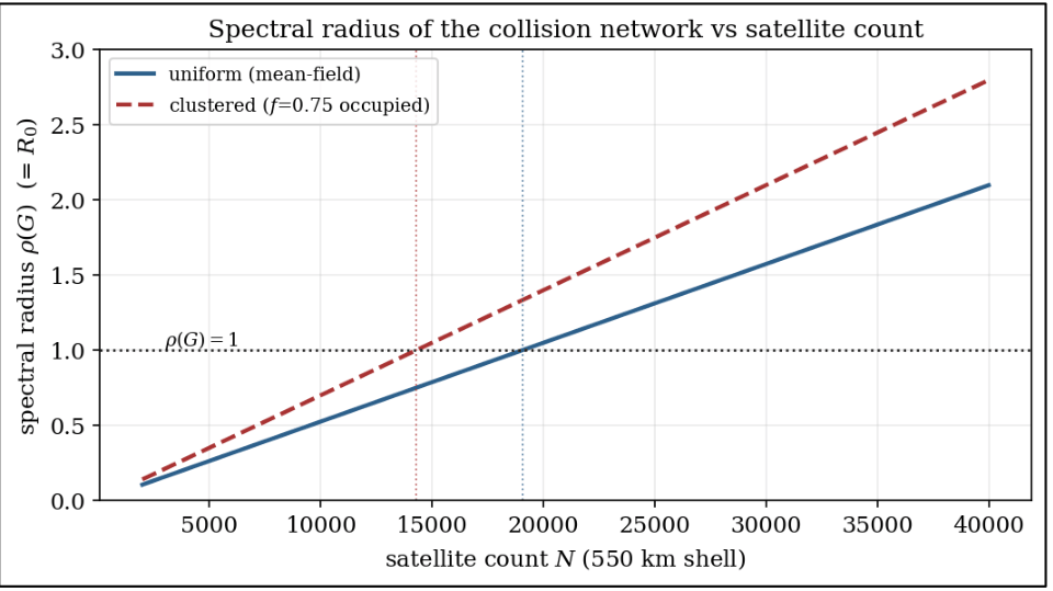
The network used to generate Figure 4 was constructed as follows. For each satellite count N, orbital elements were sampled at fixed semi-major axis corresponding to the 550 km shell and near-circular eccentricity, with inclination and right ascension of the ascending node drawn uniformly over the shell for the spatially uniform case, and assigned to discrete orbital planes following Walker-Delta and Street-of-Coverage geometries for the clustered case. Because each matrix entry already integrates the encounter rate over the debris residence time 1/δ, the matrix is evaluated at a single epoch rather than propagated step by step; temporal information enters through the factor 1/δ rather than through explicit orbit propagation. Two objects were treated as sharing a local volume V, and therefore joined by an edge, when their orbits approach within a separation comparable to the shell thickness H; pairs separated by more than this distance contribute negligibly to the encounter rate and were assigned zero weight, which sets the edge cutoff. The resulting matrix is sparse, and its leading eigenvalue was obtained by power iteration rather than by dense decomposition, which is what makes the large-N evaluations in Figure 4 tractable.

The stability criterion follows from the theory of next-generation matrices used to define epidemic thresholds²². The system is unstable when the spectral radius G of this matrix exceeds unity:

When G exceeds 1, collision risk can essentially “percolate” across the network: a single collision can trigger a cascade that propagates through the graph, which is a percolation-type transition. Because G equals the reproduction number R₀ for a uniform shell, this criterion is exactly consistent with the differential-equation threshold R₀=1, while additionally capturing spatial clustering. This mirrors the use of spectral bounds by Rechner and Berger (2016) for Markov-chain state graphs, and extends Acciarini et al. (2023), who modelled LEO collision risk as a network of conjunction events and showed that strong spatial clustering within orbital planes can raise the effective conjunction rate well above mean-field predictions^19,23.

Results

Analytical Instability Threshold

By applying canonical 550 km parameter values to the instability condition, a quantitative critical threshold can be produced. The values used are representative of the shell targeted by the Starlink constellation: a collision cross-section σ=10m² (accounting for solar-panel deployment), a mean relative velocity vᵣₑₗ=10km/s , a shell thickness H=50km, and a debris decay rate δ=0.20 per year, corresponding to an orbital lifetime of approximately five years at 550 km. These give a collision coefficient α≡σvᵣₑₗ/H=2.0m²s⁻¹ (equivalently 6.3×10⁷m²yr⁻¹). Substituting into the instability condition R₀=αβρₛ/δ=1 gives the critical product:

The threshold R₀=1 marks the point where the system shifts from stable to unstable behavior: below it the debris population stays bounded, and above it, debris production outpaces removal and the population grows without bound. Taking a nominal fragment yield β=100 gives a critical areal density ρₛ,crit≈3.2×10⁻¹¹m⁻², which for the 550 km shell corresponds to a satellite population of order 19,000 to 20,000. The threshold responds smoothly to the parameters: increasing the collision cross-section σ by 50% (representing larger next-generation satellites) reduces the critical density by about one-third, while halving the decay rate (representing higher-altitude orbits with weaker atmospheric drag) halves the critical density, since ρₛ,crit is proportional to δ.

Sensitivity Analysis

Because the absolute satellite count depends on several uncertain parameters, its sensitivity was examined by varying each input across a plausible range while holding the others at their nominal values. The critical count scales inversely with the fragment yield and the collision cross-section , and linearly with the decay rate : varying β from 50 to 1,000 moves the threshold from roughly 38,000 down to about 1,900 satellites; varying from 0.10 to 0.40 per year moves it from about 9,500 to 38,000; halving or doubling the shell thickness H moves it from about 9,500 to 38,000; and varying the relative velocity from 7 to 14 km/s moves it from about 27,000 to 13,600. Across these single-parameter variations the critical count spans roughly an order of magnitude in each direction, from a few thousand to a few tens of thousands of satellites. The robust conclusions are therefore the dimensionless structure of the threshold and the existence and location of the R₀=1 bifurcation; the absolute count should be read as an order-of-magnitude estimate that requires calibration against high-fidelity models before being used to set hard limits. A further caveat is that this analysis varies each parameter in isolation, whereas several are physically coupled: the areal density ρₛ and the fragment yield β are not independent, since denser deployments and shared collision-avoidance infrastructure can alter the effective per-collision fragment production. Joint variation of correlated parameters could therefore displace the threshold relative to the one-at-a-time estimates reported here.

Monte Carlo Simulation Results

The Monte Carlo simulations are in close agreement with the analytical prediction. Below the threshold (R₀<1) essentially no trial produced a runaway: across 10,000 trials per configuration the estimated probability of a debris cascade was statistically indistinguishable from zero, with debris populations either declining or fluctuating around a low, bounded level.

Above the threshold the probability of a cascade rises steeply with R₀. The estimated runaway probability increases from about 0.05 at R₀=1.05 (95% confidence interval roughly ±0.004) to 0.39 at R₀=1.1, 0.78 at R₀=1.2, 0.91 at R₀=1.4, and effective certainty (above 0.99) by R₀=2. Confidence intervals were obtained from the binomial standard error over the 10,000 trials together with batch-to-batch variation, and are at the level of a few tenths of a percent. Once initiated, a cascade sometimes followed a dormant period in which no collision occurred by chance before accelerated debris accumulation began.

The simulations also reveal a feature absent from the deterministic model: a transition zone, roughly R₀ ∈ [1.06,1.37] (about 20,000 – 26,000 satellites at nominal parameters), within which stable and unstable outcomes coexist probabilistically and the cascade probability climbs from near zero to near one. This zone is approximately 30% wide in R₀, indicating that the analytical threshold is best understood as the centre of a probabilistic transition rather than a sharp line. Figure 3 shows this behavior.

Graph-Theoretic Analysis: Spectral Radius Transition

The graph-theoretic analysis provides the most geometrically realistic view of the instability transition. As satellite density is increased in the simulated 550 km shell constellation, the spectral radius G of the next-generation matrix increases monotonically. For a spatially uniform shell the transition G=1 coincides exactly with the analytical threshold R₀=1 derived from the differential-equation model, because the two quantities are algebraically identical; spatial clustering then shifts the transition to lower satellite counts.

The spectral radius analysis also reveals that when satellites are non-uniformly distributed, the instability threshold is lowered by nearly 20 to 30 percent relative to the mean-field prediction. Clustered configurations, which arise naturally from the orbital mechanics of Walker-Delta and Street-of-Coverage constellation geometries, are more vulnerable than those that are more evenly distributed. The spectral-radius curve in Figure 4 makes the percolation-like transition more concrete.

Discussion

Synthesis of Model Results

The key finding of these four complementary frameworks is their convergence on a stability condition despite their fundamentally different mathematical structures. The Markov chain model, the differential equation system, the Monte Carlo stochastic simulation, and the graph-theoretic spectral analysis all converge on the threshold ρₛ · β ≈ 3.2 × 10⁻⁹ m⁻² as the boundary between stable and Kessler-like behavior. The four frameworks make different assumptions about spatial uniformity, temporal resolution, and their randomness, yet because they share a common mean-field description, their agreement is best understood as an internal consistency check rather than independent confirmation, and the specific numerical values remain subject to the uncertainties inherent in these simplified assumptions. This threshold is also broadly consistent with more advanced models such as Sturza and Saura Carretero’s 2021 analysis, where they identified that the onset of the Kessler-like cascade at collision parameters and failure rates that fall within the upper end of the stability zone identified here. Thus, despite there being two different approaches, which were built on different assumptions and mathematical structures, they both converge on the same dangerous region of parameter space¹⁰.

Furthermore, all four frameworks conclude that the increase in satellite areal density ρₛ is a dominant factor in crossing the instability threshold, with the debris-generation rate β acting as a multiplicative amplifier. This sensitivity was reinforced in 2026 by Mackintosh et al., who found that at 750 km and 98 degrees inclination, a 0.5 meter resolution Earth observation satellite faces a collision probability of 1.3×10-2, which is roughly 1.6 times the value at the same altitude but equatorial inclination (0 degrees)³. These magnitudes sit squarely within the sensitivity ranges that were predicted by the analytical model. Similar trends have also appeared in recent collision-risk studies of mega-constellations, which showed that planned constellation deployments create an alarming increase in conjunction probabilities even prior to full scale deployments. This shows that the current deployment trajectories are approaching the marginal stability zone. 

This has important implications for responsibility distribution. Roughly speaking, debris-generation rate is an aspect of satellite construction and operational procedures that can be influenced by engineering choices. For example, satellites can be designed to minimize fragmentation in the event of a collision, and operational procedures can minimize the risk of catastrophic events. Conversely, satellite density is a direct function of regulatory decisions about how many satellites each operator is permitted to deploy. This finding thus places primary responsibility for orbital sustainability on regulatory authorities rather than exclusively on individual operator engineering choices.

This attribution should be read as an interpretation of the model’s structure rather than a direct model output. The only strictly quantitative result is that the areal density ρₛ enters the stability condition as the dominant term; the mapping of ρₛ onto regulatory decisions and of onto operator engineering is an interpretive step, and the separation is imperfect, since operator design also influences and the collision-avoidance behavior embedded in the effective decay rate. The conclusion is therefore best understood as identifying the single largest lever on stability rather than as removing responsibility from operators.

Orbital Stability Regime Map

Translating the analytical threshold into operational terms, a stability regime map can be constructed that classifies the LEO system into three distinct regimes based on satellite areal density and debris-generation rate. Table 1 summarizes the key stability regimes identified across all four modeling frameworks, with the satellite counts assuming that the 550 km shell’s surface area is approximately 6.02×10⁸ km² 6.02×10¹⁴ m².

Stability Regime	Areal Density (ρₛ)(m⁻²)	Debris Rate (β)		Approx. Satellite Count (550 km)
Stable	ρₛ<3.2×10⁻¹¹	< 100 fragments		< 20,000
Marginal	3.2-6.3×10⁻¹¹	100–500 fragments		20,000 – 38,000
Unstable (Kessler-like)	ρₛ>6.3×10⁻¹¹	> 500 fragments		> 38,000

In this stable regime, all four models agree that the debris population remains bounded, and perturbations decay back toward the debris-free state. In the marginal regime, spanning densities between 3.2×10⁻¹¹ and 6.3×10⁻¹¹ m⁻², long-term stability is sensitive to specific parameter combinations and stochastic fluctuations. Monte Carlo simulations demonstrate that a small fraction of trials, typically 10 to 30 percent, evolve toward debris-dominated outcomes even when mean-field predictions suggest marginal stability. The unstable regime, characterized by densities above approximately 6.3×10⁻¹¹ m⁻² consistently produces Kessler-like behavior across all modeling approaches.

It is important to note that the relationship between satellite areal density and absolute satellite count depends on the surface area of the orbital shell. For a 550 km altitude shell (radius approximately 6,921 km), the spherical surface area is approximately 6.02 × 10⁸ km² , or 6.02×10¹⁴ m². Converting the density thresholds accordingly, a satellite count of 20,000 corresponds to an areal density of approximately 3.3×10⁻¹¹ m⁻², while 40,000 satellites correspond to 6.6×10⁻¹¹ m⁻². These numbers must be compared not to the total surface area of the sphere but to the effective area accessible within the constellation’s orbital planes, which is smaller and makes the effective density substantially higher than the spherical average suggests.

Furthermore, Cheng et al. (2023) demonstrated that when managing satellite constellations, it is imperative to not simply rely on the satellites acting independently. To retain a smooth operation, the satellites must make coordinated multi-agent decisions, rather than functioning as independent systems⁵. This same conclusion is applied to managing space debris. Object accumulation in the marginal zone can only be averted if the entire constellation coordinates its collision-avoidance actions, which is precisely the type of multi-satellite and system wide approach that newer early warning and monitoring systems have begun to develop.

Comparison with Existing Literature

The quantitative thresholds derived here are broadly consistent with and, in several respects, extend the warnings found in the existing peer-reviewed literature with greater specificity. Boley and Byers (2021) demonstrated using simplified models that untracked debris would lead to dangerous collisions on a regular basis due to the large number of satellites in mega-constellation orbital shells, and subsequently highlighted the inadequacy of existing regulatory frameworks⁷. Their analysis, while failing to identify a specific critical density threshold, characterized the problem qualitatively with terms that are consistent with our quantitative findings. Furthermore, Zhang et al. (2022) found that collision risk increases were alarming, even at planned deployment levels, corroborating our finding that existing planned constellations are operating near or within the marginal stability regime¹⁷.

Reiland et al. (2021) demonstrated the importance of how Minimum Space Occupancy (MiSO) orbital configurations could significantly reduce endogenous collision risk with nearly indistinguishable adjustments to nominal orbital elements²⁴. This finding is complementary to our graph-theoretic result that spatial distribution strongly influences the instability threshold, and suggests that constellation design optimization could push the effective instability threshold higher by reducing spatial clustering. Appel’s (2024) MOCAT-MC analysis reaches consistent conclusions about exponential population growth at higher LEO altitudes and impending exceedance of critical density thresholds¹⁶. What the present paper provides that MOCAT-MC cannot is an explicit, closed-form expression for the instability threshold and a multi-framework validation of that expression using analytically transparent methods accessible to the greater populations. 

Policy Implications

The analytical framework developed here has several direct and actionable policy implications. Firstly, the numerical limits on constellation size at specific altitude bands are the most directly available regulatory tool, and the results here provide a scientific basis for establishing them. Current regulatory frameworks in the United States, Europe, and elsewhere focus primarily on end-of-life disposal requirements but do not impose hard limits on total constellation size. The quantitative thresholds identified here, being approximately 20,000 satellites as the upper bound of the stable regime and 38,000 as the onset of unstable dynamics in the 550 km altitude band, provide a scientific basis for establishing such numerical limits.

Secondly, the mandatory deorbit timeline is a critical policy parameter. A deorbit requirement of five years, now mandated by both the U.S. Federal Communications Commission and ESA, increases the effective debris decay rate by a factor of roughly five relative to the previous 25-year norm, substantially expanding the safe operating regime²¹. This result quantitatively validates the policy of the five-year rule and argues strongly for international adoption of equivalent standards.

Third, active debris removal (ADR) technologies can be represented in our model as an increase in the effective debris decay rate δ. Jaekel et al.’s (2018) robotic capture methodology and Takahashi’s (2025) plasma beam approach represent complementary removal technologies suited to different debris types^13,14. Even modest ADR rates can increase meaningfully at current debris population levels. However, our model also reveals a critical warning: if constellation deployment increases faster than debris mitigation efforts, the system can transition into the unstable regime before ADR technologies are mature enough to compensate. The race between deployment velocity and mitigation capacity is thus a key determinant of long-term orbital sustainability.

Lastly, the graph-theoretic’s finding that spatial clustering lowers the effective instability threshold by 20 to 30 percent highlights the importance of orbital architecture in determining instability risk. International coordination on frequency and orbital slot allocation, currently managed through the International Telecommunication Union (ITU), could be extended to include requirements for minimum spacing between orbital planes of competing constellations, reducing the spatial clustering that lowers the effective instability threshold. Furthermore, the findings indicate that a constellation’s instability risk isn’t simply determined by how many satellites it contains, but rather how spread out those satellites are across orbital planes and altitudes as well. Designs that pack large numbers of satellites into a few planes are more prone to instability than systems that distribute satellites more evenly. These findings are further informed with Acciarini et al. (2023), who showed that the conjunction rates are underestimated when observations are sparse, largely due to the fact that objects tend to cluster within specific orbital regimes²³. 

Model Strengths and Limitations

The primary strength of the modeling framework presented here is its analytical transparency. Every equation, assumption, and parameter in the model is explicitly stated and can be independently evaluated by any researcher. The framework is also computationally accessible: the Markov chain and differential equation analyses can be performed with basic mathematical software, and the Monte Carlo simulation, while more demanding, requires only modest computational resources and is implementable in open-source programming environments. This accessibility makes the framework valuable not only as a research tool but as an educational resource for emerging researchers and a communication tool for engaging policymakers who lack specialized computational infrastructure.

The limitations of the framework are equally important to acknowledge. The most significant is the assumption of spatial uniformity in the mean-field models. Since real constellations are not uniformly distributed across the orbital shell but are rather concentrated in discrete orbital planes with specific inclinations, the mean-field models presented in this analysis can potentially create local density enhancements that can substantially exceed the shell-averaged density. The graph-theoretic component partially addresses this limitation by capturing inter-satellite proximity explicitly, but it too relies on simplified geometric assumptions about orbital geometry. Second, the model does not account for altitude-dependent atmospheric drag driven by the solar cycle, in which solar activity modulates the density of the upper atmosphere and hence the orbital decay rate of debris. Third, the model treats collision outcomes using a simplified debris-generation model and does not capture the full fragmentation mass distribution predicted by the NASA Standard Breakup Model²⁵. Lastly, the differential equation model assumes that the satellite population S(t) is held approximately constant by ongoing launches, which is a reasonable approximation for mature constellations but may not hold during rapid deployment phases.

A further and important limitation is that all four frameworks share the same mean-field assumption, so their agreement reflects internal consistency rather than independent validation. Mean-field treatment also tends to over-predict collisions, because it ignores orbital structure and active collision avoidance; the effective collision coefficient should therefore be regarded as an upper bound and the thresholds as conservative. The clear priority for future work is external calibration and validation: comparing the threshold and the transition zone against observed conjunction statistics and against established debris-evolution tools such as NASA’s LEGEND, ESA’s MASTER, and MIT’s MOCAT-MC before the absolute satellite counts are used to set hard regulatory limits^26,27,28,29.

Conclusion

This paper set out to identify at what combination of satellite density and debris-generation rate a LEO mega-constellation becomes dynamically unstable. The answer, derived from four complementary analytical frameworks, including a Markov chain analysis, coupled differential equation modeling, Monte Carlo stochastic simulation, and graph-theoretic spectral analysis, is a consistent critical instability threshold. The product of satellite areal density and debris-generation rate per collision must remain below approximately δ/α≈3.2×10⁻⁹m⁻² (equivalently R₀=1) under canonical 550 km parameters to maintain stable dynamics. In operational terms, this constitutes a stable regime below approximately 20,000 satellites, a marginal zone from approximately 20,000 to 38,000 satellites, and a dynamically unstable regime above approximately 38,000 satellites, assuming the absence of aggressive debris mitigation efforts.

Several features of this analysis are worth restating. The convergence of all four frameworks on the same threshold is the central result; because the frameworks share a mean-field description, however, this convergence is an internal consistency check rather than independent confirmation. Satellite density is the dominant stability parameter, which places primary regulatory responsibility at the institutional level rather than distributing it entirely to individual operators through engineering requirements. The roughly 30-percent-wide stochastic transition zone argues against treating the threshold as a line to approach asymptotically. The 20 to 30 percent reduction in effective threshold caused by spatial clustering has direct implications for how constellation orbital architectures should be designed and regulated. And the connection between the analytical delta parameter and active debris removal technologies grounds the abstract mathematics in concrete engineering decisions.

The orbital environment is a commons, or a shared global resource, and like all commons, it is susceptible to tragedy when individual actors pursue their self-interests without coordination mechanisms in place. The mathematical analysis presented here demonstrates that this tragedy is not a distant hypothetical but a threshold that current deployment trajectories are approaching within decades. Preventing it requires not merely good intentions from individual operators, but a coordinated international regulatory response grounded in the quantitative understanding that this and related research is beginning to provide. The tools of probabilistic modeling and dynamical systems analysis are available, and the only thing that remains is the institutional will to act on them.

Acknowledgments

I would like to extend my deepest gratitude to my mentor, Sanjay Ganachari Nagaraja, for his valuable guidance and insightful feedback throughout the creation of this paper.

References

1. M. M. Bennett, Z. Cudney. Holding up the skies: is Starlink occupying low Earth orbit? Territory, Politics, Governance. 2026, https://doi.org/10.1080/21622671.2025.2594491. [↩] [↩] [↩]
2. S. Haritwal. LEO satellite mega-constellations: market dynamics, orbital mechanics, policy challenges, and the future of global connectivity. SSRN Working Paper, Next Move Strategy Consulting. 2025, https://ssrn.com/abstract=5450454. [↩]
3. J. Mackintosh, K. Smith, C. McGrath. Collision risk from performance requirements in Earth observation mission design. Advances in Space Research. Vol. 77, pg. 5941–5961, 2026, https://doi.org/10.1016/j.asr.2026.01.019. [↩] [↩] [↩]
4. F. Farhangian, R. Landry, Jr. Multi-constellation software-defined receiver for Doppler positioning with LEO satellites. Sensors. Vol. 20, pg. 5866, 2020, https://doi.org/10.3390/s20205866. [↩]
5. Y. Cheng, C. Wei, S. Sun, B. You, Y. Zhao. An LEO constellation early warning system decision-making method based on hierarchical reinforcement learning. Sensors. Vol. 23, pg. 2225, 2023, https://doi.org/10.3390/s23042225. [↩] [↩]
6. H. Chen, H. Yu, H. Zhang, H. Chen, X. Kong, H. Li, D. Qing. Low Earth orbit satellite switching and recovery method based on generic congestion control algorithm. Scientific Reports. Vol. 15, pg. 25341, 2025, https://doi.org/10.1038/s41598-025-10649-z. [↩]
7. A. C. Boley, M. Byers. Satellite mega-constellations create risks in low Earth orbit, the atmosphere and on Earth. Scientific Reports. Vol. 11, pg. 10642, 2021, https://doi.org/10.1038/s41598-021-89909-7. [↩] [↩] [↩]
8. A. Choueiri. Electromagnetic active debris removal: scalable solutions for orbital sustainability and Kessler Syndrome mitigation. Preprint, TechRxiv. 2026. [↩] [↩] [↩]
9. Z. Shareefdeen, H. Al-Najjar. Pollution effects and management of orbital space debris. ACS Omega. Vol. 9, pg. 5127–5141, 2024, https://doi.org/10.1021/acsomega.3c07462. [↩] [↩] [↩]
10. M. A. Sturza, G. Saura Carretero. Mega-constellations: a holistic approach to debris aspects. Proceedings of the 8th European Conference on Space Debris. ESA Space Debris Office, 2021. [↩] [↩] [↩] [↩]
11. D. J. Kessler, B. G. Cour-Palais. Collision frequency of artificial satellites: the creation of a debris belt. Journal of Geophysical Research: Space Physics. Vol. 83, pg. 2637–2646, 1978, https://doi.org/10.1029/JA083iA06p02637. [↩] [↩] [↩]
12. J. Hudson. KESSYM: a stochastic orbital debris model for evaluation of Kessler Syndrome risks and mitigations. Preprint, New Trier High School, 2022. [↩] [↩] [↩] [↩]
13. S. Jaekel, R. Lampariello, W. Rackl, M. De Stefano, N. Oumer, A. M. Giordano, O. Porges, M. Pietras, B. Brunner, J. Ratti, Q. Muehlbauer, M. Thiel, S. Estable, R. Biesbroek, A. Albu-Schaeffer. Design and operational elements of the robotic subsystem for the e.deorbit debris removal mission. Frontiers in Robotics and AI. Vol. 5, pg. 100, 2018, https://doi.org/10.3389/frobt.2018.00100. [↩] [↩] [↩]
14. K. Takahashi. Cusp-type bi-directional radiofrequency plasma thruster toward contactless active space debris removal. Scientific Reports. Vol. 15, pg. 30589, 2025, https://doi.org/10.1038/s41598-025-16449-9. [↩] [↩] [↩]
15. P. D. Anz-Meador, J. N. Opiela, J.-C. Liou. History of on-orbit satellite fragmentations, 16th edition. NASA/TP-20220019160, NASA Orbital Debris Program Office, Houston, TX, 2023. [↩] [↩] [↩]
16. G. F. Appel. Low Earth orbit stability analysis using Monte-Carlo techniques. Master’s thesis, Massachusetts Institute of Technology, MIT Department of Aeronautics and Astronautics, 2024. [↩] [↩] [↩] [↩]
17. Y. Zhang, B. Li, H. Liu, J. Sang. An analysis of close approaches and probability of collisions between LEO resident space objects and mega constellations. Geo-spatial Information Science. Vol. 25, pg. 104–120, 2022, https://doi.org/10.1080/10095020.2022.2031313. [↩] [↩]
18. Y. Tao, Y. Guo, S. Wang, C. Yu, Z. Zhu. Satellite selection strategy and method for signals of opportunity navigation and positioning with LEO communication satellites. Sensors. Vol. 25, pg. 267, 2025, https://doi.org/10.3390/s25010267. [↩]
19. S. Rechner, A. Berger. Marathon: an open source software library for the analysis of Markov-chain Monte Carlo algorithms. PLOS ONE. Vol. 11, pg. e0147935, 2016, https://doi.org/10.1371/journal.pone.0147935. [↩] [↩] [↩]
20. C. J. Maddison. A Poisson process model for Monte Carlo. Perturbation, Optimization, and Statistics. pg. 193–232, 2016. [↩]
21. M. M. Bennett. Orbital debris requires prevention and mitigation across the satellite life cycle. Communications Engineering. Vol. 4, pg. 95, 2025, https://doi.org/10.1038/s44172-025-00430-5. [↩] [↩]
22. O. Diekmann, J. A. P. Heesterbeek, M. G. Roberts. The construction of next-generation matrices for compartmental epidemic models. Journal of the Royal Society Interface. Vol. 7, pg. 873–885, 2010, https://doi.org/10.1098/rsif.2009.0386. [↩]
23. G. Acciarini, N. Baresi, C. Bridges, L. Felicetti, S. Hobbs, A. Gunes Baydin. Observation strategies and megaconstellations impact on current LEO population. Proceedings of the 2nd NEO and Debris Detection Conference (NEOSST2). University of Surrey, 2023. [↩] [↩]
24. N. Reiland, A. J. Rosengren, R. Malhotra, C. Bombardelli. Assessing and minimizing collisions in satellite mega-constellations. Advances in Space Research. Vol. 67, pg. 3755–3774, 2021, https://doi.org/10.1016/j.asr.2021.01.010. [↩]
25. N. L. Johnson, P. H. Krisko, J.-C. Liou, P. D. Anz-Meador. NASA’s new breakup model of EVOLVE 4.0. Advances in Space Research. Vol. 28, pg. 1377–1384, 2001, https://doi.org/10.1016/S0273-1177(01)00423-9. [↩]
26. J.-C. Liou, N. L. Johnson. Instability of the present LEO satellite populations. Advances in Space Research. Vol. 41, pg. 1046–1053, 2008, https://doi.org/10.1016/j.asr.2007.04.081. [↩]
27. D. Jang, D. D’Ambrosio, M. Lifson, P. Pasiecznik, R. Linares. Stability of the LEO environment as a dynamical system. Advanced Maui Optical and Space Surveillance Technologies (AMOS) Conference, 2022. [↩]
28. D. D’Ambrosio, S. Servadio, P. M. Siew, R. Linares. Novel source-sink model for space environment evolution with orbit capacity assessment. Journal of Spacecraft and Rockets. Vol. 60, 2023, https://doi.org/10.2514/1.A35579. [↩]
29. M. Lifson, D. D’Ambrosio, C. Arnas, R. Linares. How many satellites can we fit in low Earth orbit? Capacity integrating risk-based and intrinsic methods. AAS/AIAA Astrodynamics Specialist Conference, 2022. [↩]