Investigating Frequency-Band Contributions and Temporal Data Leakage in EEG Eye-State Classification

Abstract

Electroencephalography (EEG) is widely used to classify eye states, and alpha-band activity (8-13 Hz) has traditionally been regarded as the dominant predictor because it peaks when the eyes are closed. However, it remains unclear whether alpha activity alone is sufficient, or whether information relevant to eye-state classification is distributed across the broader EEG spectrum. This study investigates whether alpha-band activity is the sole critical predictor of EEG-based eye state classification under both Random Split and Time Aware Split conditions.  Causal band filtering was applied to the UCI EEG Eye State dataset to produce band-isolated and band-suppressed feature sets across the Alpha, Beta, and Theta frequency bands, and an XGBClassifier was evaluated under both splits, with  permutation and ablation tests used to assess statistical significance across frequency band conditions and different splits. All experimental conditions performed below the mean majority-class baseline and statistical testing indicated non-significance in sufficiency and necessity (all p ≥ 0.156, all 95% CIs include 0). While Random splitting seemed to result in noticeably inflated performance, exemplified by 3 conditions which outperformed the mean majority-class baseline, statistical testing via unpaired permutation test showed otherwise (all p ≥ 0.468). These findings suggest that no single frequency band serves as the sole predictor of eye-state and a non-significant difference between training protocols during EEG eye state classification.

Keywords: Neuroscience, Computational Neuroscience, EEG, XGBoost, Machine Learning

Introduction

Electroencephalography (EEG) is a non-invasive method used to measure electrical activity in the brain with high temporal resolution. As a portable process and as a sensor that’s sensitive to rapid neural changes, it is commonly used for studies on brain states and neural dynamics performed under cognitive thinking, sleep, or eye state^1,2.

The Berger effect is characterized by a noticeable increase in alpha band power (8–13 Hz) upon eye closure^3,4,5,6. This connection has made alpha-band activity a prime focus in EEG-based eye state classification^7,8 and is also why there is often widespread consideration of eye state as a control variable for alpha-band activity in EEG analysis⁹.

However, it remains unclear whether alpha-band activity alone is sufficient to distinguish eye states or whether other frequency bands also provide critical information to classification performance. EEG signals are inherently broadband, and frequency bands such as Beta (13–30 Hz) and Theta (4–8 Hz) are also known to reflect distinct cognitive and physiological processes^10,11.

Accordingly, the main hypothesis in this study is that while alpha-band activity is important, information relevant to eye-state classification is distributed across multiple frequency bands.

To investigate, we assessed the contributions of different EEG frequency bands to eye-state classification by comparing band-isolated and band-suppressed conditions across Alpha, Beta, and Theta bands along with the baseline.

This study aims to test whether selectively removing a given frequency band from the signal degrades classification performance more than retaining its isolated counterpart, thereby providing evidence about the relative criticality of each band.

Furthermore, this study examines the effect of evaluation protocol on classification performance. Due to the continuous nature of EEG data, during EEG ML training, models often learn predictable background timing patterns rather than actual brain signals, leading to artificially inflated accuracy scores^12,13,14,15.

By contrasting the results of the random split, which retains all temporal data leakage, and the time-aware split, designed to mitigate the effects¹⁶, this study also aims to assess the extent to which evaluation methodology affects classification performance in EEG and machine learning research.

Methods

Research Design

This study is a single-subject (n=1), single-session, retrospective secondary analysis of a previously-collected EEG recording¹⁷, incorporating both a within-signal ablation design (band isolation vs suppression) and a controlled comparison of evaluation protocols (random vs time-aware splitting).

Dataset Preparation

Dataset was obtained from the UCI Machine Learning Repository (EEG Eye State, dataset ID 264), originally released by Rösler & Suendermann (2013) at http://suendermann.com/corpus/EEG_Eyes.arff.gz¹⁷.

The dataset consists of 14,980 EEG measurements recorded over 117 seconds from a single participant using an Emotiv EEG Neuroheadset. Each sample contains 14 different EEG channel readings (AF3, F7, F3, FC5, T7, P7, O1, O2, P8, T8, FC6, F4, F8, AF4) along with a target label (eyeDetection), where 1 indicates eyes closed and 0 indicates eyes open. Eye state annotations were manually added by analyzing simultaneous video recordings.

The original authors removed 3 out of 14,980 measurements due to obvious transmission errors, leaving 14,977. We applied our own independent z-score-based exclusion procedure (|z| > 6), resulting in 4 flagged instances (indices 898, 10386, 11509, 13179) in near agreement with the original preprocessing. The measurements were subsequently deleted from our analysis, as a result, yielding 14,976 measurements.

Causal Band Filtering

To investigate the role of specific EEG frequency bands in eye state classification, a causal band filter was applied to make two feature sets per band: one where the target frequency band has been isolated and one where it has been suppressed.

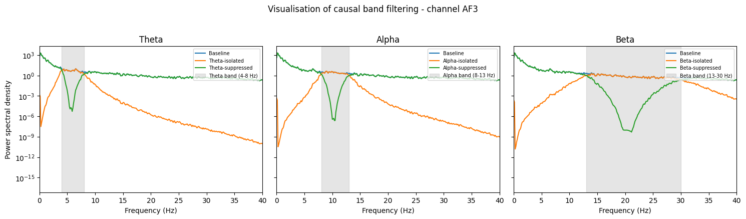
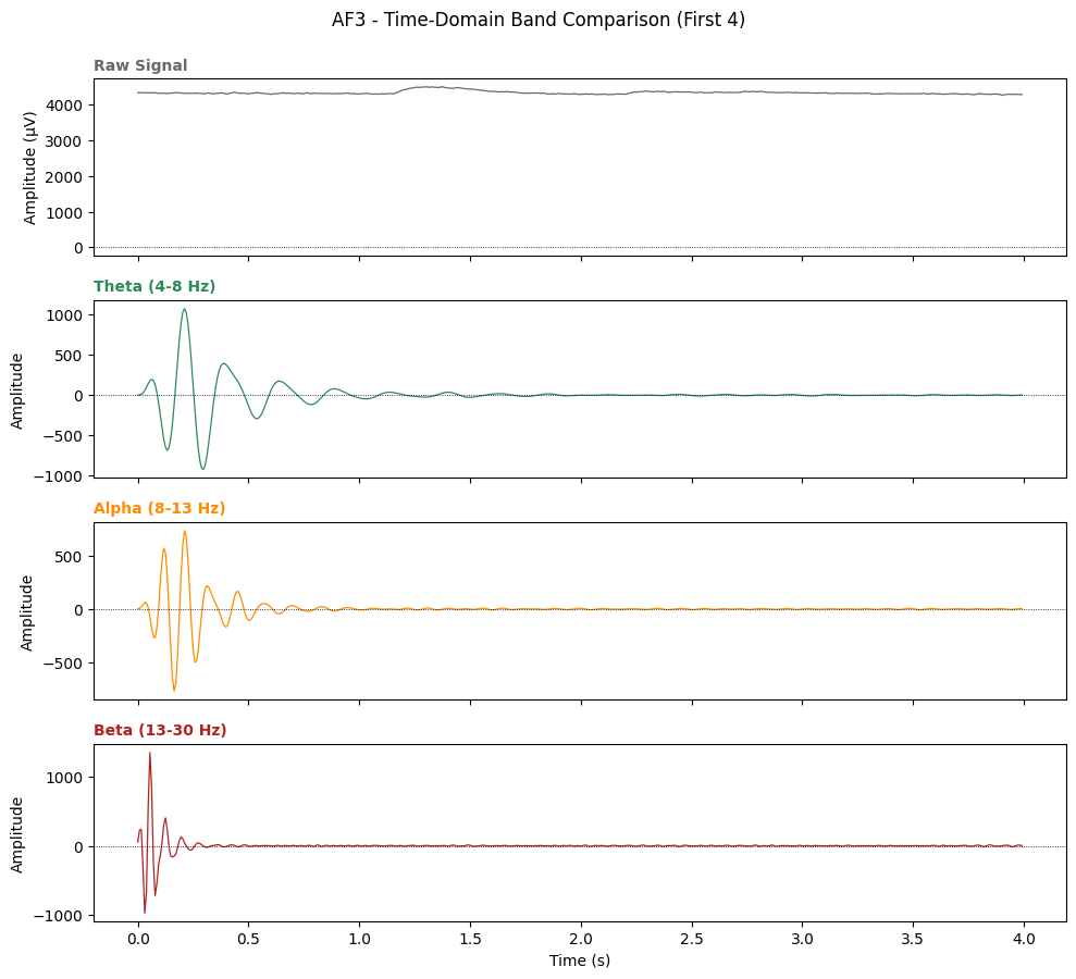
To isolate or suppress a target frequency band, we replaced full-record frequency masking with a causal fourth-order Butterworth filter¹⁸ (scipy.signal.butter), applied via (scipy.signal.lfilter). Because a causal filter’s output at time t depends only on inputs at times ≤ t, a single filtering pass over each channel cannot introduce information from later, held-out time periods into earlier training samples¹⁹.

While the original paper does not report an explicit value in Hz²⁰, we took the sampling rate to be 128 Hz, consistent with the manufacturer-specified sampling rate of the Emotiv EPOC headset²¹ used in the original recording and the corpus’s own reported duration and sample count (14,980 instances ÷ 117 s ≈ 128 Hz).

Band-isolated signals were produced with a bandpass filter and band-suppressed signals were produced with a bandstop filter. As shown in Figures 1 and 2, frequency bands were correctly defined as Alpha (8-13 Hz), Beta (13–30 Hz), and Theta (4-8 Hz).

Windowing and Feature Extraction

Each condition’s filtered signal was segmented into non-overlapping 1.5s windows (192 raw samples per window or 78 windows per condition). For each window and channel, we computed a log band-power feature as the log of the mean squared amplitude within that window²², rather than treating each 1/128s sample as an independent observation.

window_sec	condition	n_windows_total	n_windows_usable	n_folds_used	mean_accuracy	sd_accuracy	mean_balanced_accuracy	mean_f1	mean_majority_class_baseline
1	Baseline	117	98	5	0.55	0.092702	0.54881	0.456835	0.675
1	Alpha-Isolated	117	98	5	0.525	0.055902	0.540675	0.398697	0.675
1	Alpha-Suppressed	117	98	5	0.55	0.149217	0.547024	0.506273	0.675
1.5	Baseline	78	59	5	0.555556	0.136083	0.590635	0.433553	0.8
1.5	Alpha-Isolated	78	59	5	0.4	0.168508	0.359048	0.233333	0.8
1.5	Alpha-Suppressed	78	59	5	0.533333	0.182574	0.577302	0.425674	0.8
2	Baseline	58	40	5	0.533333	0.074536	0.54	0.487619	0.8
2	Alpha-Isolated	58	40	5	0.366667	0.298142	0.4	0.477143	0.8
2	Alpha-Suppressed	58	40	5	0.533333	0.074536	0.54	0.487619	0.8
2.5	Baseline	46	28	5	0.5	0.306186	0.45	0.438095	0.85
2.5	Alpha-Isolated	46	28	5	0.3	0.410792	0.25	0.342857	0.85
2.5	Alpha-Suppressed	46	28	5	0.6	0.379144	0.55	0.504762	0.85
3	Baseline	39	21	5	0.6	0.365148	0.533333	0.52	0.866667
3	Alpha-Isolated	39	21	5	0.466667	0.380058	0.416667	0.46	0.866667
3	Alpha-Suppressed	39	21	5	0.6	0.365148	0.533333	0.52	0.866667

Window length was selected via a sensitivity sweep across 1.0-3.0s (Table 1), using the Alpha frequency band as a representative for the 2 others. As shown, the usable window count decreased with window length (98, 59, 40, 28, 21 windows), while fold-level accuracy variance grew dramatically when beyond 2.0s. Based on this, we selected a window length of 1.5s as the point before this variance increase, prioritizing estimated stability over the window length that happened to yield the highest accuracy for any single condition.

Windows overlapping an eye-state transition were excluded from modeling, 19 out of 78 windows (24.4%) being dropped for each band.

Evaluation Protocols

Two evaluation protocols were applied to the windowed, band-power feature set described above: random split and time-aware split.

In the random split, the feature set was divided into training and test sets via an 80/20 stratified split, repeated across five random seeds (0,1,2,3,4) to reduce sensitivity to any single partition.

In the time-aware split, as shown in Table 2, we used TimeSeriesSplit with five folds and an explicit two-window (3s) gap between the end of each training partition and the start of its corresponding test partition, preventing near-boundary window overlap. Both protocols operate on the identical windowed, causally-filtered features, which is what makes their results directly comparable for the first time in this analysis.

The number of folds as 5 reflects a tradeoff between per-fold test-set size and the granularity needed for the permutation test described below.

Because TimeSeriesSplit training sets grow with each fold, training-set size varied roughly four-fold across folds (ranging 12-48 across 5 usable folds). We treat this as a scope limitation on any claim attributing the random-vs-time-aware accuracy gap solely to leakage.

Fold	Train windows	Train duration	Test windows	Test duration	Gap (windows)
1	0-11 (12)	0-18.0s	14-22 (9)	21.0-34.5s	2
2	0-20 (21)	0-31.5s	23-31 (9)	34.5-48.0s	2
3	0-29 (30)	0-45.0s	32-40 (9)	48.0-61.5s	2
4	0-38 (39)	0-58.5s	41-49 (9)	61.5-75.0s	2
5	0-47 (48)	0-72.0s	50-58 (9)	75.0-88.5s	2

Classification Model

XGBoost’s XGBClassifier version 3.2.0 was utilized for binary classification of the eye state label. XGBoost is a gradient boosting framework²³ that builds an ensemble of decision trees sequentially, with each tree correcting the residual errors of its predecessors²⁴ The model was trained separately on each experimental condition with the same hyperparameters.

The hyperparameters applied are as follows. The model was configured with 100 estimators (boosting rounds), providing sufficient capacity to capture complex patterns, without excessive computational power needed. A learning rate of 0.1 was selected to ensure more gradual convergence across boosting rounds, reducing the risk of overfitting to any single tree’s errors. A maximum tree depth of 5 was chosen to allow the model to capture moderately complex feature interactions while preventing individual trees from overfitting to noise in the EEG signal, given the inherently variable nature of EEG data. XGBoost was instructed to perform binary classification by predicting probabilities (objective = ‘binary:logistic’), evaluate accuracy using log loss (eval_metric = ‘logloss’), and maximize training speed by leveraging every CPU core available (n_jobs = -1). Finally, the random state was fixed at 42 to ensure reproducibility.

Moreover, Numpy version 2.4.1, Scipy version 1.17.0, Scikit-learn version1.8.0 were utilised throughout the experiment^25,26,27.

Statistical Testing

Two statistical tests were performed on the perceived mean accuracies: unpaired and paired permutation test.

To determine whether the observed performance drop under time-aware evaluation is statistically significant, we perform a two-sided independent-samples permutation test²⁷ (R = 9,999 resamples). Under the null hypothesis that evaluation protocol has no effect on performance accuracy, we pooled the performance scores from both protocols, repeatedly shuffled them into two surrogate groups, and recalculated the difference in means. The resulting p-value represents the proportion of differences that equal or exceed the observed gap, with p < 0.05 denoting a statistically significant evaluation bias.

On the other hand, to evaluate whether individual frequency bands were sufficient or necessary for prediction, each experimental condition was compared with the baseline model using a paired permutation test across the cross-validation folds.

Within the paired permutation test, two hypotheses were examined by testing whether the model trained with a specific frequency band saw a significant decrease in performance. First, for isolated-band conditions a significant decrease would indicate that band alone was insufficient in matching the performance of the baseline; and a non-significant result would indicate that the test did not by itself establish sufficiency. Second, for suppressed-band conditions, the test would assess the necessity of the band that was suppressed. In both cases, a one-sided alternative hypothesis (`alternative = ‘less’`) was specified beforehand, corresponding to the hypothesis that the experimental condition would produce lower accuracy than the baseline.

The said statistical test was performed using SciPy’s paired permutation test (`scipy.stats.permutation_test`) with (permutation_type=’samples’). As only five paired cross-validation folds were available, the test employed exact permutation enumeration (n_resamples = np.inf) rather than random resampling. With five paired observations, there are 2⁵ = 32 possible sign-flip arrangements, allowing every permutation to be evaluated thoroughly. Consequently, the smallest attainable exact two-sided p-value is 2/32 = 0.0625, indicating that, with this experimental design, statistical significance at the conventional p = 0.05 level cannot be achieved. Because this floor already exceeds the conventional single-comparison threshold, no additional correction for multiple comparisons was applied across the six band-condition comparisons performed; results are accordingly interpreted as descriptive rather than confirmatory. We also note that TimeSeriesSplit folds share overlapping training data by construction, with each successive fold’s training set being a superset of the previous fold’s, so the five folds do not constitute fully independent observations, and the permutation test’s exchangeability assumption should be read with this dependency in mind.

For each comparison, the mean paired difference in classification accuracy between the model trained under experimental conditions and the baseline model was calculated and reported. In addition, a 95% confidence interval for the mean paired difference was estimated using Student’s t-distribution and the confidence interval’s upper and lower limits were reported to avoid ambiguity in the results. To ensure valid paired comparisons, analyses were restricted to folds available in both the baseline and experimental conditions whenever unequal numbers of usable folds occurred.

Necessity Ablation

To further evaluate the necessity of each frequency band, the band-suppressed conditions were compared with the baseline conditions via a necessity ablation test. While it corresponds with one of the statistical test hypotheses stated above, the test was performed following the recommendation that these represent separate questions rather than two halves of one experiment.

Both models were evaluated on identical windowed segments and cross-validation folds. Because window exclusion (dropping windows that straddle an eye-state transition) depends only on the shared label sequence and window length and not on the band-filtered signal itself, the full-spectrum and band-suppressed conditions produce identically ordered, identically indexed window sequences by construction; as a safeguard, label correspondence was verified explicitly before comparison, and any length mismatch would have restricted the comparison to the shared leading window sequence.

A significant result (p < 0.05, one-sided) indicates the removed band contributed meaningfully to classification performance. A non-significant result indicates the test did not detect such a contribution at this sample size (five folds); and again, given the exact test’s minimum attainable p-value of 0.0625 two-sided, this should be read as inconclusive rather than as evidence the band is unimportant.

Evaluation Metric

Simple classification accuracy alone can fail to show class-specific error when there’s an imbalance. Therefore, balanced accuracy, being the mean of per-class recall, along with the F1 / Precision / Recall triplet were reported as the results and summarized on a table.

Per-condition results are summarized as the mean of each metric across folds or seeds (accuracy additionally reported with SD), alongside the mean majority-class baseline for direct comparison; confusion matrices are summed element-wise across folds/seeds into one aggregate matrix per condition and reported as raw counts with row-normalized percentages.

Results

Time-Aware Split

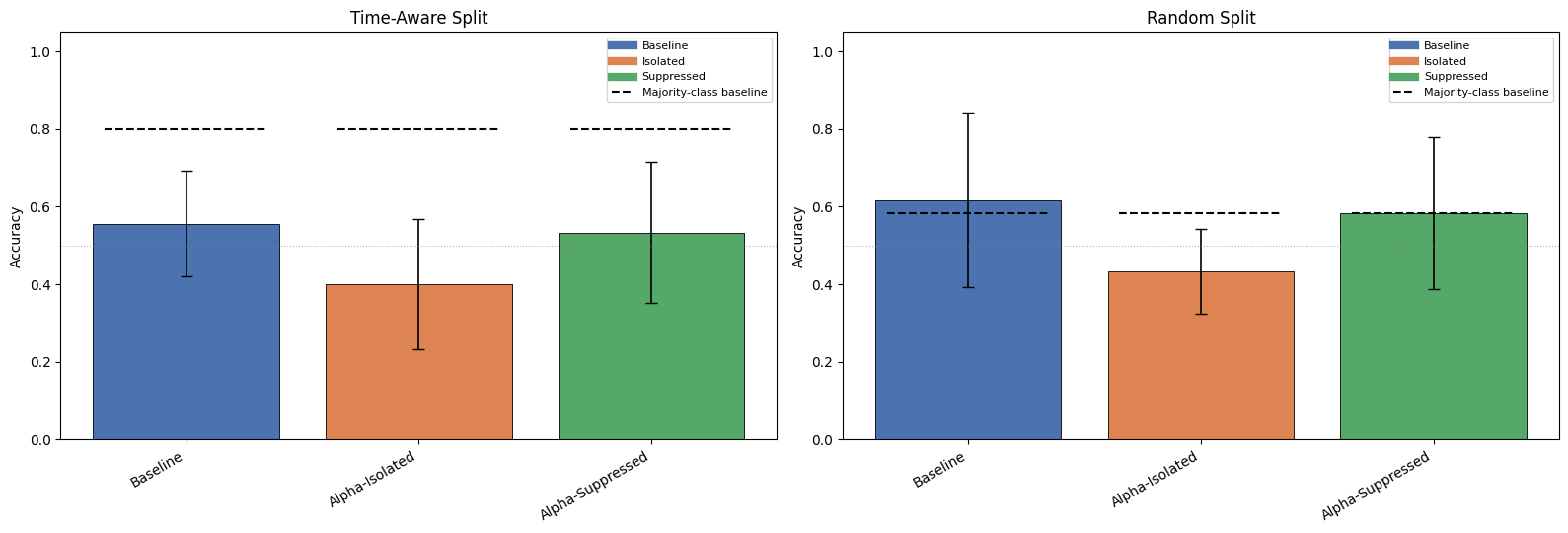
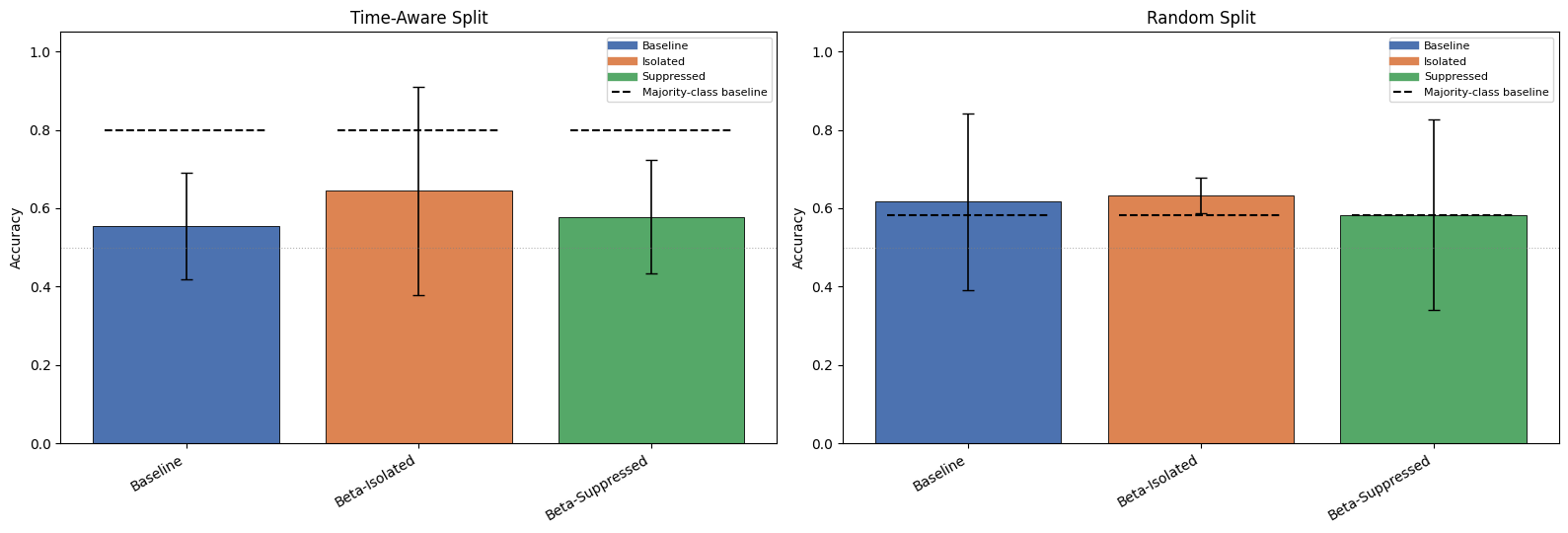
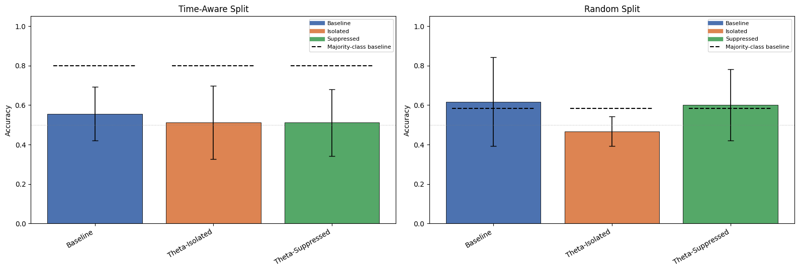
Within the Time-Aware split results (Table 3), experimental conditions had accuracies hovering around the mid mark, while the majority-class baseline was fixed at 0.8.

The Beta-Isolated condition had the highest mean accuracy (0.644) while the Alpha-Isolated condition had the lowest (0.4), each one of the 7 conditions sitting below the 0.800 majority-class baseline. The largest gap being in Alpha-Isolated (−0.400), the smallest gap being in Beta-Isolated (−0.156).

Condition	n_folds_used	mean_accuracy	sd_accuracy	mean_balanced_accuracy	mean_f1	mean_precision	mean_recall	mean_majority_class_baseline
Baseline	5	0.533333	0.074536	0.54	0.487619	0.483333	0.633333	0.8
Alpha-Isolated	5	0.4	0.168508	0.359048	0.233333	0.313333	0.233333	0.8
Alpha-Suppressed	5	0.533333	0.182574	0.577302	0.425674	0.420952	0.588889	0.8
Beta-Isolated	5	0.644444	0.265274	0.709841	0.502222	0.43	0.7	0.8
Beta-Suppressed	5	0.577778	0.144871	0.610635	0.445674	0.44	0.588889	0.8
Theta-Isolated	5	0.511111	0.185924	0.543968	0.462597	0.430952	0.6	0.8
Theta-Suppressed	5	0.511111	0.168508	0.557302	0.413553	0.406667	0.588889	0.8

Random Split

Contrary to the Time-Aware split (Table 3), several conditions with accuracies exceeding 0.6 could be seen (Baseline, Beta-Isolated, Theta-Suppressed) and the majority-class baseline was fixed at far lower (0.583) for Random split (Table 4). As such, the Baseline, Alpha-Suppressed, Beta-Isolated and Theta-Suppressed conditions outperformed the majority-class baseline.

But similarly to the Time-Aware Split, Beta-Isolated had the highest mean accuracy at 0.633 while Alpha-Isolated had the lowest at 0.433.

Condition	n_folds_used	mean_accuracy	sd_accuracy	mean_balanced_accuracy	mean_f1	mean_precision	mean_recall	mean_majority_class_baseline
Baseline	5	0.616667	0.225154	0.585714	0.447619	0.55	0.4	0.583333
Alpha-Isolated	5	0.433333	0.108653	0.422857	0.321399	0.295	0.36	0.583333
Alpha-Suppressed	5	0.583333	0.195434	0.551429	0.39974	0.506667	0.36	0.583333
Beta-Isolated	5	0.633333	0.045644	0.617143	0.52022	0.573333	0.52	0.583333
Beta-Suppressed	5	0.583333	0.242956	0.551429	0.410649	0.526667	0.36	0.583333
Theta-Isolated	5	0.466667	0.074536	0.462857	0.384371	0.363889	0.44	0.583333
Theta-Suppressed	5	0.6	0.180662	0.571429	0.432727	0.493333	0.4	0.583333

Accuracy by Band

Figures 3 to 5 show mean accuracy with standard-deviation error bars for each band, alongside its own majority-class baseline, under both evaluation protocols.

Unpaired Permutation Test

As a result of the unpaired statistical test in Table 5, it can be seen that for the differences observed between the Time-Aware and Random splits, all condition’s achieved a p-value of 0.468 or above Theta-Suppressed being the lowest at said mean accuracy. Notably, both Beta bands had a p-value of 1.0.

condition	mean_diff	pvalue
Baseline	0.061111	0.603175
Alpha-Isolated	0.033333	0.777778
Alpha-Suppressed	0.05	0.785714
Beta-Isolated	-0.011111	1
Beta-Suppressed	0.005556	1
Theta-Isolated	-0.044444	0.690476
Theta-Suppressed	0.088889	0.468254

Paired Permutation Test

None of the conditions reached a p-value below the standard of p<0.05, which is expected given the 0.0625 two-sided floor at n=5 folds. Every 95% confidence interval range crossed the 0.0 mark. Finally, noticeably, Alpha-Isolated has the numerically largest effect (−0.156) and smallest p-value (0.156) out of the 6 (Table 6).

condition	n_folds	n_arrangements	mean_diff	alternative	pvalue_exact	ci_lower	ci_upper
Alpha-Isolated	5	32	-0.155556	less	0.15625	-0.473169	0.162058
Alpha-Suppressed	5	32	-0.022222	less	0.5	-0.173353	0.128908
Beta-Isolated	5	32	0.088889	less	0.75	-0.254635	0.432413
Beta-Suppressed	5	32	0.022222	less	1	-0.039477	0.083921
Theta-Isolated	5	32	-0.044444	less	0.46875	-0.429753	0.340864
Theta-Suppressed	5	32	-0.044444	less	0.5	-0.167842	0.078953

Necessity Ablation Test

As seen in Table 7, the necessity ablation test results came out to be the same as the necessity test via the suppressed band paired permutation test performed above (Table 6).

condition	n_folds	n_arrangements	mean_diff	alternative	pvalue_exact	ci_lower	ci_upper
Alpha-Suppressed	5	32	-0.022222	less	0.5	-0.173353	0.128908
Beta-Suppressed	5	32	0.022222	less	1	-0.039477	0.083921
Theta-Suppressed	5	32	-0.044444	less	0.5	-0.167842	0.078953

Confusion Matrices

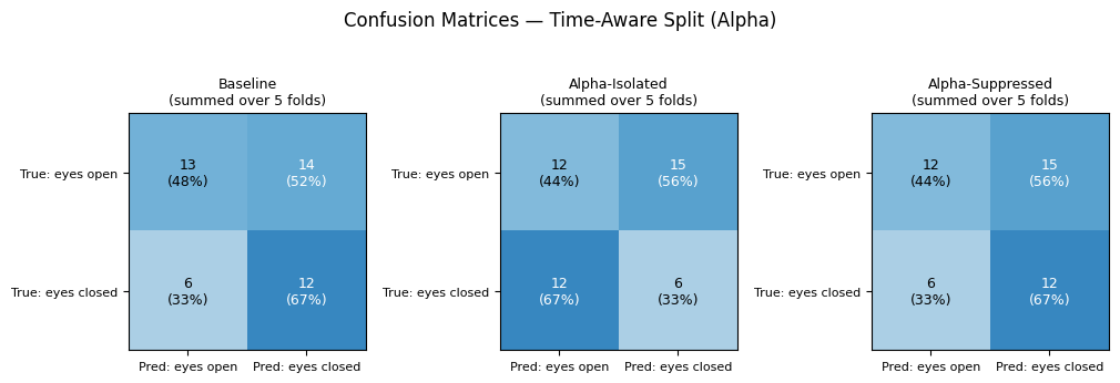
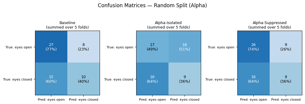
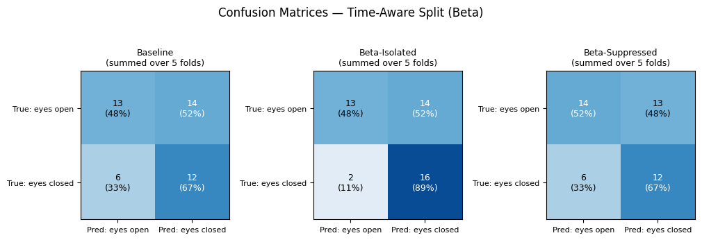
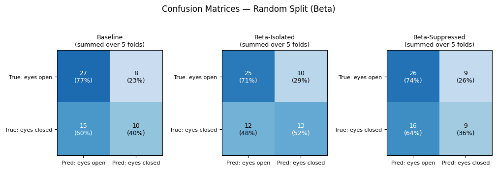
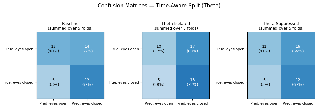
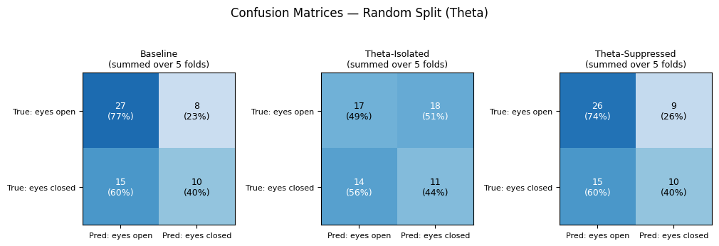
Confusion matrices for all seven conditions under both evaluation protocols are shown in Figures 6 to 11.

Per-class recall was not stable across evaluation protocol for any of the three bands’ isolated conditions. For Beta-Isolated, eyes-closed recall was 88.9% under time-aware but 52.0% under random-split, while eyes-open recall showed the opposite pattern (48.1% time-aware vs. 71.4% random). Alpha-Isolated and Theta-Isolated showed smaller but similar shifts between protocols. Under time-aware, Alpha-Isolated recall fell below 50% for both classes simultaneously (44.4% eyes-open, 33.3% eyes-closed), performing worse than chance-level guessing on each class individually rather than only on average.

Discussion

Headline Finding

The primary hypothesis under examination in this revision is that no single frequency band (Alpha, Beta, or Theta) is independently necessary nor sufficient for eye-state classification. Two findings in this study support this hypothesis.

First, across all seven conditions evaluated under time-aware validation, classification accuracy fell below the corresponding fold-wise majority-class baseline (Table 3). This gap was largest for Alpha-Isolated, where mean accuracy (ΔM=-0.400), and smallest for Beta-Isolated (ΔM=0.156). The key finding here is that even the best-performing condition did not exceed the performance of always predicting the majority class within each fold.

Second, as can be seen in Table 6 and Table 7, none of the six paired sufficiency and necessity analysis reached statistical significance (all p ≥ 0.156), and all six confidence intervals passed through zero.

The result and the key finding of this experiment is therefore accurate to the original hypothesis.

Band Specific Interpretations

More information regarding frequency band contributions can be obtained via statistical testing in each frequency condition.

None of the six paired comparisons in Table 6 (three sufficiency tests isolated band vs. baseline and three necessity tests suppressed band vs. baseline) reached the (p ≤ 0.05) threshold, and every 95% confidence interval passed through zero. Under a paired exact permutation test with five folds, the minimum achievable two-sided p-value is 0.0625, so this design is not suitable to detect small-to-moderate effects; a non-significant result here indicates that the test did not detect a difference, not that no difference exists. Therefore, none of the three bands are interpreted as either critical or unimportant to eye-state classification performance. The three bands are more appropriately described as inconclusive.

Among the six comparisons, the alpha-isolated sufficiency test produced the numerically largest effect and smallest p-value (ΔM = −0.156, p = 0.156, 95% CI [−0.473, 0.162]), making it the most suggestive of the six results. With the beta-suppressed, on the other hand, the necessity test produced both the smallest effect and the tightest confidence interval of the six (ΔM = 0.022, p = 1.000, 95% CI [−0.039, 0.084]), making it the least suggestive of any band-specific effect in this analysis, though not treated as evidence of an effect.

Random vs Time-Aware Comparison

Despite visible differences between the two, there are three factors contributing to the differences between random-split and time-aware accuracy, with regard to each protocol’s own majority-class-baseline (Table 3 vs Table 4).

First, causal band filtering removes the pathway by which earlier preprocessing could incorporate information from later, held-out time periods. Second, windowing removes the near-duplicate-neighbor pathway by which adjacent, highly correlated samples could previously appear on both sides of a random split.

Third, separate from either temporal leakage pathway, time-aware training-set size varied substantially across folds (12 to 48 windows, a 4.0-fold range), and the recording was non-stationary in class balance across time. Both can affect fold-wise accuracy independent of any leakage.

When that gap was tested directly via an unpaired permutation test comparing each condition’s random-split and time-aware split accuracy (Table 5), no condition reached statistical significance (all p ≥ 0.468). We therefore do not claim the leakage corrections produced a statistically confirmed reduction in accuracy.

The confusion matrices add another caution against over-interpreting the random-vs-time-aware gap as a single effect. Per-class recall for the isolated-band conditions was not consistent across protocol, and in the case of Beta-Isolated, the direction of the class-wise recall imbalance reversed entirely between the two splits. (Figures 6 – 11)

Isolated vs Suppressed

The isolated and suppressed conditions did not follow a uniform pattern relative to one another.

Suppressed outperformed isolated for alpha in both splits (Time-Aware: 0.533 vs. 0.400; Random: 0.583 vs. 0.433) and for theta in the random split (0.600 vs. 0.467), while theta was exactly tied in the time-aware split (0.511 vs. 0.511). Only Beta showed the opposite pattern in both splits, with isolated exceeding suppressed (Time-Aware: 0.644 vs. 0.578; Random: 0.633 vs. 0.583). (Figures 3 – 4)

However, where suppressed did outperform isolated, we interpret this as an expected consequence of the asymmetry between the two rather than as evidence that classification-relevant information is distributed across the broader spectrum. An isolated band retains only its own narrow bandwidth, whereas its corresponding suppressed condition retains everything outside it, including the other two canonical bands and any residual drift or artifact. Furthermore, Beta’s reverse in observation for both splits further argues against it.

Limitations

This study holds several limitations. First, the dataset used was collected from one participant in one recording session, leaving it unknown how broadly these findings can be applied. Second, our z-score-based exclusion criterion (|z| > 6) flagged four anomalous samples rather than the three removed by Rösler and Suendermann (2013). We report this discrepancy rather than adjusting the threshold to match the original count. Third, the Butterworth filters used to isolate and suppress each band have a gradual slope rather than a sharp cutoff (Figures 1 and 2); the results should be interpreted with this in mind. Fourth, all results reported are from a single classifier configuration (as per the hyperparameters described in the methodology); the results should therefore not be generalized to other model classes. Finally, no artifact-rejection or line-noise treatment was applied beyond the causal band filtering itself, and that suppressed-band conditions in particular may retain external electrical activity alongside neural signals; we cannot rule out that some suppressed-condition performance may reflect non-cerebral information.

It is also important to note that classification accuracy may not fully capture differences in model performance across conditions.

Future Work

Future studies could replicate this methodology across multiple participants and mutiple recording sessions to allow the finding reported here to be extended to generalization across individuals. Artifact-rejection could be applied to rule out external sources of electrical activity especially within the suppressed-band conditions. A channel or regional level ablation such as comparison between posterior and anterior electrode groups would extend the frequency only comparison to test whether specific regions, rather than or in addition to specific frequency bands, contribute to classification performance.

Finally, repeating the necessity and sufficiency comparisons with a regularized linear classifier alongside XGBoost would test whether the inconclusive band-specific results reported here are a property of the underlying data or specific to gradient-boosted tree ensembles.

Conclusion

In conclusion, this study evaluated whether Alpha, Beta, or Theta band EEG activity when independent is necessary or sufficient for eye-state classification via the UCI EEG Eye State dataset. Under the time-aware evaluation, no experimental condition exceeded its corresponding majority-class baseline and no frequency band showed statistically significant sufficiency or necessity. These results therefore are accurate to the original hypothesis that no single frequency band is independently critical to eye-state classification, nor is any frequency band disposable. We further show that random split and time-aware split do not differ significantly in accuracy for any of the seven experimental conditions. This opposes any claim, in this work or in future work using this dataset, that a specific accuracy gap between evaluation protocols is evidence of leakage rather than a descriptive pattern consistent with several possible contributing factors.

References

1. Y. Roy, H. Banville, I. Albuquerque, A. Gramfort, T. H. Falk, & J. Faubert. Deep learning-based electroencephalography analysis: A systematic review. Journal of Neural Engineering, 16(5), 051001, 2019. [↩]
2. F. Lotte, L. Bougrain, A. Cichocki, M. Clerc, M. Congedo, A. Rakotomamonjy, & F. Yger. A review of classification algorithms for EEG-based brain–computer interfaces: A 10 year update. Journal of Neural Engineering, 15(3), 031005, 2018. [↩]
3. C. Han, C. Yao, Y. Wang, S. Li, Y. Yao, X. Liu, K. Zhang, & C. Zhang. Localization of the Berger effect in human posterior brain regions with simultaneous electroencephalogram (EEG) and stereo-EEG (SEEG) recordings. NeuroImage, 327, 121748, 2026. [↩]
4. W. Hohaia, B. W. Saurels, A. Johnston, K. Yarrow, & D. H. Arnold. Occipital alpha-band brain waves when the eyes are closed are shaped by ongoing visual processes. Scientific Reports, 12, 1194, 2022. [↩]
5. R. J. Barry, A. R. Clarke, S. J. Johnstone, C. A. Magee, & J. A. Rushby. EEG differences between eyes-closed and eyes-open resting conditions. Clinical Neurophysiology, 118(12), 2765–2773, 2007. [↩]
6. W. Klimesch. EEG alpha and theta oscillations reflect cognitive and memory performance: A review and analysis. Brain Research Reviews, 29(2–3), 169–195, 1999. [↩]
7. E. Yosrita, Y. Heryadi, & L. Lukas. Eye state classification using EEG based on electrode position. In 2018 International Conference on Applied Science and Technology (iCAST), 2018. [↩]
8. T. Wang, S.-U. Guan, K. L. Man, & T. O. Ting. EEG eye state identification using incremental attribute learning with time-series classification. Mathematical Problems in Engineering, 2014, 365101, 2014. [↩]
9. O. Jensen & A. Mazaheri. Shaping functional architecture by oscillatory alpha activity: Gating by inhibition. Frontiers in Human Neuroscience, 4, 186, 2010. [↩]
10. A. K. Engel & P. Fries. Beta-band oscillations—signalling the status quo? Current Opinion in Neurobiology, 20(2), 156–165, 2010. [↩]
11. J. F. Cavanagh & M. J. Frank. Frontal theta as a mechanism for cognitive control. Trends in Cognitive Sciences, 18(8), 414–421, 2014. [↩]
12. X. Xu, B. Wang, B. Xiao, Y. Niu, Y. Wang, X. Wu, H. Cheng, & J. Chen. The impacts of temporal autocorrelations on EEG decoding. Biomedical Signal Processing and Control, 113, 108783, 2026. [↩]
13. S. Kapoor & A. Narayanan. Leakage and the reproducibility crisis in machine-learning-based science. Patterns, 4(9), 100804, 2023. [↩]
14. S. Saeb, L. Lonini, A. Jayaraman, D. C. Mohr, & K. P. Kording. The need to approximate the use-case in clinical machine learning. GigaScience, 6(5), gix019, 2017. [↩]
15. G. Brookshire, J. Kasper, N. M. Blauch, Y. C. Wu, R. Glatt, D. A. Merrill, S. Gerrol, K. J. Yoder, C. Quirk, & C. Lucero. Data leakage in deep learning studies of translational EEG. Frontiers in Neuroscience, 18, 1373515, 2024. [↩]
16. Butterworth, S. (1930). On the theory of filter amplifiers. Experimental Wireless and the Wireless Engineer, 7, 536–541 [↩]
17. O. Rösler & D. Suendermann. A first step towards eye state prediction using EEG. In Proceedings of the AIHLS 2013, International Conference on Applied Informatics for Health and Life Sciences, 2013. [↩] [↩]
18. S. Butterworth. On the theory of filter amplifiers. Experimental Wireless and the Wireless Engineer, 7, 536–541, 1930. [↩]
19. P. Virtanen, R. Gommers, T. E. Oliphant, M. Haberland, T. Reddy, E. Cournapeau, E. Burovski, P. Peterson, P. Weckesser, J. Bright, S. J. van der Walt, M. Brett, J. Wilson, J. Millman, K. J. Mayorov, A. Nelson, R. J. Jones, R. Kern, E. Larson, … SciPy 1.0 Contributors. SciPy 1.0: Fundamental algorithms for scientific computing in Python. Nature Methods, 17, 261–272, 2020. [↩]
20. O. Rösler & D. Suendermann. A first step towards eye state prediction using EEG. In Proceedings of the AIHLS 2013, International Conference on Applied Informatics for Health and Life Sciences, 2013. [↩]
21. M. Duvinage, T. Castermans, M. Petieau, T. Hoellinger, G. Cheron, & T. Dutoit. Performance of the Emotiv Epoc headset for P300-based applications. BioMedical Engineering OnLine, 12, 56, 2013. [↩]
22. P. D. Welch. The use of fast Fourier transform for the estimation of power spectra: A method based on time averaging over short, modified periodograms. IEEE Transactions on Audio and Electroacoustics, 15(2), 70–73, 1967. [↩]
23. J. H. Friedman. Greedy function approximation: A gradient boosting machine. The Annals of Statistics, 29(5), 1189–1232, 2001. [↩]
24. T. Chen & C. Guestrin. XGBoost: A scalable tree boosting system. In Proceedings of the 22nd ACM SIGKDD International Conference on Knowledge Discovery and Data Mining (KDD ’16), pp. 785–794, Association for Computing Machinery, 2016. [↩]
25. F. Pedregosa, G. Varoquaux, A. Gramfort, V. Michel, B. Thirion, O. Grisel, M. Blondel, V. Prettenhofer, R. Weiss, V. Dubourg, V. Vanderplas, A. Passos, A. Cournapeau, M. Brucher, M. Perrot, & É. Duchesnay. Scikit-learn: Machine learning in Python. Journal of Machine Learning Research, 12, 2825–2830, 2011. [↩]
26. C. R. Harris, K. J. Millman, S. J. van der Walt, R. Gommers, P. Virtanen, T. Cournapeau, E. Wieser, J. Taylor, B. Berg, N. J. Smith, R. Kern, M. Picus, M. Hoyer, M. H. van Kerkwijk, M. Brett, A. Haldane, J. F. del Río, M. Wiebe, M. Peterson, … K. J. Oliphant. Array programming with NumPy. Nature, 585, 357–362, 2020. [↩]
27. J. D. Hunter. Matplotlib: A 2D graphics environment. Computing in Science & Engineering, 9(3), 90–95, 2007. [↩]