Rhythmicity Index: Signifying Shape Consistency in Addition to Phase Consistency

Abstract

The Q-factor, calculated from the power spectrum, is a common identifier of oscillation in neural and excitable-media signals, yet it does not guarantee that the shape of the wave repeats. In fact, on a simulated signal generator based on the Greenberg–Hastings excitable model on Erdős–Rényi networks with N = 20,000 and mean degree K = 200, we found that among 125,000 runs, signals with the sharpest spectral peaks seldom produce repeated waveforms. We therefore introduce the Rhythmicity Index, which considers two factors simultaneously: phase consistency, whether peaks occur at a regular interval, and shape consistency, whether the waveform repeats across cycles. The Rhythmicity Index shows minimum correlation with the Q-factor (Spearman ρ = −0.005), as well as the fact that all 120 top-percentile Q-factor runs scored RI below the rhythmic threshold that we set. To verify the effectiveness of RI, we implemented it on real human EEG data from 20 subjects, dividing the signals into 600 four-second epochs across conditions. RI successfully reproduces the Berger effect in all 15 artifact-free subjects by showing higher values in the eyes-closed groups than the eyes-open groups, with a Cohen’s d_z = 1.42. We acknowledge that RI is not a total replacement for the Q-factor; however, when a spectral peak can either result from a genuine oscillation or broadband noise, the Q-factor fails to distinguish them, but RI can by examining the waveform directly as a safeguard.

Keywords: rhythmicity, neural oscillations, power spectrum, Q-factor, waveform shape, excitable networks, EEG, Berger effect

Introduction

Rhythmic activity is a defining feature of neural systems, and quantifying it correctly underpins most claims about brain dynamics. When distinguishing rhythmic from arrhythmic signals, one common classifier is the Q-factor^1,2, which is calculated by dividing a peak’s center frequency by its bandwidth. The Q-factor has one key defect, however: it does not guarantee that the shape of the wave repeats.

Academia has probed into the effectiveness of the Q-factor through three different angles. On detection: reliable detection requires separating a spectral peak from the background spectrum’s own structure³; single-trial characterization is acutely sensitive to estimator choices spectral summaries hide⁴; and the current standard, spectral parameterization (specparam)^5,6, calls a peak oscillatory only once the aperiodic 1/f-like background is accounted for. On transience: many putative “rhythms” are transient bursts⁷, and the rate of brief high-power beta events, not sustained amplitude, predicts behavior^8,9. On waveform shape: a rhythm’s waveform carries physiological information spectral summaries discard, motivating cycle-by-cycle analysis^10,11; beta-waveform sharpness asymmetries track pathology and treatment state in Parkinson’s disease¹²; source-to-sensor projection distorts waveform shape¹³; within-cycle instantaneous-frequency profiles characterize waveform dynamics directly¹⁴; and non-sinusoidal waveforms leak harmonic power into higher bands, so apparent beta rhythms can be alpha-band waveform shape in disguise^15,16. Fransen, van Ede, and Maris¹⁷ proposed detecting oscillations by their rhythmicity, the regularity of recurrence, rather than by spectral power alone.

Demonstrating this directly requires many varied, inspectable signals, which empirical recordings do not provide at scale, so we use a stochastic excitable network as a controlled signal generator of thousands of activity time series, from silent to noisy to genuinely oscillatory. The model is not offered as realistic brain tissue and we claim no new physics; its only role is to supply diverse signals whose repetition can be inspected directly.

The network belongs to the Greenberg–Hastings class¹⁸, studied extensively as an abstraction of excitable media and neural tissue¹⁹; its collective dynamics are well characterized, including the extinct–active transition²⁰, the role of the refractory period²¹, self-sustained oscillations in excitable Erdős–Rényi networks²², and transitions to absorbing states in stochastic-neuron networks^23,24: the predictions against which the generator is checked. The contribution of this paper is not about the model itself but about how we should interpret the data the model provides. The paper shows that the Q-factor falsely signifies noise as truly rhythmic, introduces RI as the solution, and validates RI on human EEG data.

Methods

Model

We simulate a stochastic three-state excitable system of the Greenberg–Hastings type¹⁸ on undirected Erdős–Rényi random networks^25,26 with N = 20,000 nodes and mean degree K = 200. Nodes are Resting, Firing, and Refractory; and all nodes evolve simultaneously, so that when a node Fires it enters a Refractory state at the next timestep, when it is Refractory there is a probability β (the recovery probability) that it resets to be Resting at the end of the timestep, otherwise it remains Refractory, and when it is in a Resting state it will Fire if any of the m currently Firing nodes are connected to it with the probability

where is the per-edge firing probability. We start with a single node being Firing, and the observable is the number of Firing nodes versus time, A(t).

Our experiments consisted of running a sweep across five independent network realisations (each specified by a different graph seed, 12345–16345 in steps of 1000). For each network, we chose five initial seed nodes (the original-analysis node plus four drawn uniformly at random). Each network and seed-node realisation was swept across a set of α parameters (25 choices from 10⁻³ to 1, logarithmically spaced by factors of 10^0.125) and a range of β values (20 choices linearly spaced from 0.05 to 1.00 in steps of 0.05). Both α and β are no-unit, dimensionless parameters. For a given network and seed node, we ran 10 simulation replicates using different deterministically derived seeds. The seed depends on the network, the initial seed node, α, β, and the run’s number among the ten replicates (1st, 2nd, and so on). In total, the simulation yields 5 networks × 5 initial seed nodes × 25 α values × 20 β values × 10 replicates per grid point = 125,000 runs. Each run has T = 2,500 timesteps. The measured window is from t = 500 to t = 2000. Additionally, 42,800 out of 125,000 (34.2% of the total) died out before the window’s end, which left 82,200 survivors.

We did not exclude any parameter configuration by default; however, in the simulation, we found that all 5,000 runs with α = 1 went extinct. This was because at α = 1, all the resting neighbors of a firing node deterministically fire at the next step, which in turn causes a massive refractoriness afterward. At β = 1.00, while runs do not go extinct on a large scale, most runs undergo a firing–refractory–resting three-timestep cycle. The period is too short to measure the waveform; hence, only 203 of 4,105 surviving runs were admissible for RI measurement.

Spectral Q-factor baseline

For each surviving run we estimated the PSD of A(t) with Welch’s method²⁷ (SciPy²⁸), specified completely because the Q-factor is sensitive to every setting: Hann window, nperseg = 256, 50% overlap, constant (mean) detrending, density scaling. On the 1,500-step window used throughout this averages ten segments at a resolution of Δf_bin = 1/256 ≈ 0.0039 cycles per timestep. The dominant peak is the largest local maximum of the PSD (scipy.signal.find_peaks; no prominence, height, or distance constraint); its center frequency f0 is refined to sub-bin resolution by parabolic interpolation on the log-PSD across the peak bin and neighbours. The Q-factor is Q=f₀/Δf, with ∆f the −3 dB (half-power) full width (half-power frequencies interpolated between bracketing bins)¹.

Two diagnostics come along with each value. For a peak narrower than three FFT bins, the width is determined by the resolution, not the signal: the estimate is flagged as resolution-limited, with the ceiling f₀/(3∆ f_bin) also given. Since the half-power width is taken from a noisy PSD (relative standard error ≈√k for an average over K segments) and appears in the denominator, the effect of noise is an upward bias of the estimated Q: estimates that average fewer than eight segments are labelled under-segmented.

The rhythmicity index

The rhythmicity index (RI) examines two factors in the time domain: whether peaks of A(t) recur at regular intervals (phase consistency) and whether the waveform repeats across cycles (shape consistency).

The repetition period

To measure both, we need the period. The period is not the dominant spectral peak, which can be a harmonic multiple of the true rate when the harmonic outpowers the fundamental. To find the true fundamental frequency, an ACF-verified subharmonic search over f0/k, k = 2 … 8, adopts the lowest of these frequencies whose autocorrelation at the corresponding lag exceeds the incumbent’s by at least 0.05 at a local maximum; its reciprocal is the period.

Phase consistency: lagged coherence

Following Fransen et al.^17,29, the mean resultant length of unit-normalized Fourier coefficients at the repetition frequency, over non-overlapping integer-cycle windows, measures window-to-window phase consistency. Two summaries are kept: the three-cycle lagged coherence c, registering locally regular rhythms even if short-lived, and the mean lagged coherence c‾, averaged over one- to ten-cycle windows, rewarding sustained consistency.

Shape consistency: cycle consistency

In the cycle-by-cycle spirit of Cole and Voytek¹¹, cycles are located by peaks and troughs (scipy.signal.find_peaks; prominence 0.3 standard deviations, minimum separation half the estimated period); segments between consecutive extrema spanning half to one and a half estimated periods are retained, resampled to the median length, and successive pairs compared by Pearson correlation. The mean cycle correlation r measures whether the waveform’s shape, not merely its timing, repeats.

Minimum sampling requirement

Shape is distinguishable from timing only with enough samples per cycle: with only three points per cycle a waveform has no measurable shape, and two random cycles then pass the shape threshold by chance far too often (null-distribution derivation in the Supporting Online Material). So we need at least eight samples per cycle and ten cycles per window: signals that do not pass either requirement are ruled inadmissible rather than scored.

Combining phase and shape

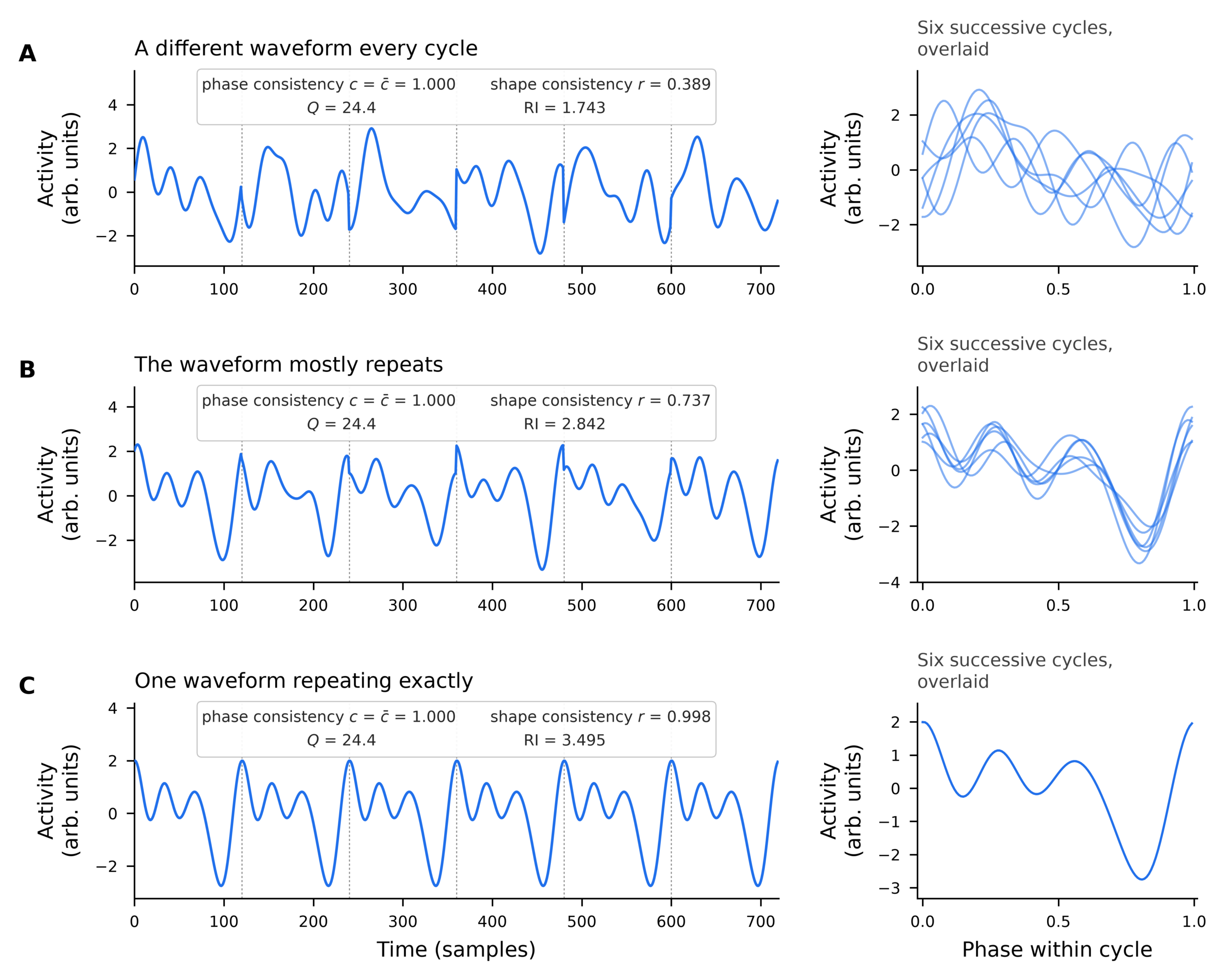
Each individual measure (c, and r) is divided by a threshold, so that a ratio ≥ 1 passes the bar; the evidence for shape, Ψ, is the cycle-correlation ratio, and the evidence for phase, Φ, is the maximum of the two coherence ratios. The main (strong) gate gs takes the weaker of the two (an AND), so regular timing with a variable waveform, or vice versa, cannot pass it (Figure 1), which makes it impossible for such signals to get high scores: the key protection against spectrally sharp noise. The secondary (weak) gate g_w separates weakly rhythmic from arrhythmic signals with looser thresholds (Φ_w, Ψ_w) and a minimum requirement for the evidence on the other dimension (Φ₀, Ψ₀, zero if the corresponding raw measure does not exceed 0.1): thus accidentally passing one criterion never leads to a higher score:

are set to 0 if the numerator .

Range

Because c, and r are bounded by 1, the strong gate is bounded by 2.5 and the rhythmic branch spans exactly [2, 3.5]. The weakly rhythmic branch uses the compressive map 2 − 1/g_w, which occupies [1, 2) and can never reach or round to 2.

The thresholds (0.5 and 0.35 for the coherence estimators, 0.4 for cycle correlation, 0.3, 0.25 and 0.2 for their looser counterparts, and the minimal-evidence floor of 0.1) are settings, not tuned constants; two are not free (the two mean-coherence thresholds derive from the weak coherence threshold t = 0.3 as max(0.35, t + 0.05) = 0.35 and max(0.20, t − 0.05) = 0.25), so the index has five independent constants, all fixed on simulated signals before the EEG data were analysed and none adjusted afterwards. The band boundaries — rhythmic (RI ≥ 2), weakly rhythmic (1 ≤ RI < 2), arrhythmic (RI < 1) — are conventional reporting cut-points. A sensitivity analysis swept the five constants ±50% one at a time: every reported conclusion held within at least −33% to +21% of each default (mostly ±40–50%), and the EEG effect stayed at d_z ≥ 1.107 with 15/15 subjects increasing throughout (Supporting Online Material, Fig. S2 and Tables S3–S5).

A worked example carrying the Figure 1B trace through every step to RI = 2.842 is in the Supporting Online Material.

EEG validation

To test generalization beyond the model, we applied the index to the Berger effect^30,31,32 (the increase in occipital alpha when the eyes close) in 20 subjects’ one-minute eyes-open (R01) and eyes-closed (R02) baseline recordings (160 Hz) from the EEG Motor Movement/Imagery Database (EEGMMIDB, PhysioNet^33,34; MNE-Python³⁵): 15 non-overlapping 4-second epochs per subject per condition, 600 total; occipital channels (O1, Oz, O2) filtered and averaged into one series before epoching.

Filtering was deliberately broad; measuring waveform shape on an already-narrowband signal would be circular: a 1–45 Hz zero-phase FIR filter (MNE-Python firwin, 529 taps, 3.31 s; Hamming window, default transition bands), each epoch’s dominant frequency estimated from its own spectrum over 3–20 Hz (not fixed to the alpha band) by the locked procedure (Welch peak, sub-bin frequency refinement on a zero-padded periodogram, ACF-verified subharmonic check), and the index computed exactly as defined, its floors at 4 s and 160 Hz admitting 2.5 Hz (ten cycles per epoch) to 20 Hz (eight samples per cycle). Control variant: the original 8–13 Hz band (a caution, not evidence).

Artifacts were excluded before any index computation by condition-blind criteria fixed in advance: EEGMMIDB has no EOG channel, so blinks were detected on the mean of Fp1, Fpz and Fp2 (1–45 Hz), rejecting epochs with a peak above 200 μV, and epochs whose maximum occipital peak-to-peak amplitude exceeded the subject’s robust threshold³⁶ (median + 4 scaled-MAD over 30 epochs, conditions pooled; subject-calibrated because a fixed cut would bias against high-amplitude occipital alpha). Rejection removed 170 of 300 eyes-open epochs (169 blink, 2 amplitude, 1 both) and 15 of 300 eyes-closed (11 blink, 4 amplitude), leaving 130 and 285 accepted, of which 365 (94 eyes-open, 271 eyes-closed) passed the admissibility floors and were scored. Five subjects retained no artifact-free eyes-open epochs, so paired statistics use the 15 with both conditions.

Effects are reported at the subject level: paired t-test on per-subject means, mean difference with 95% confidence interval, paired Cohen’s d_z, and the number of subjects increasing. Baselines on identical epochs: Q-factor, integrated 8–13 Hz log-power, cycle correlation r alone, and specparam⁵ alpha peak power (specparam 2.0.0rc7, fit to each epoch’s Welch spectrum over 3–40 Hz).

Ethical considerations

This study analyzed a publicly available, fully de-identified dataset (the EEG Motor Movement/Imagery Database, PhysioNet). Since no human participants were involved, no new EEG recordings were made, and no identifiable personal data were collected or accessed, Institutional Review Board review was not required for this secondary analysis.

Results

The generator behaves as excitable-network theory predicts

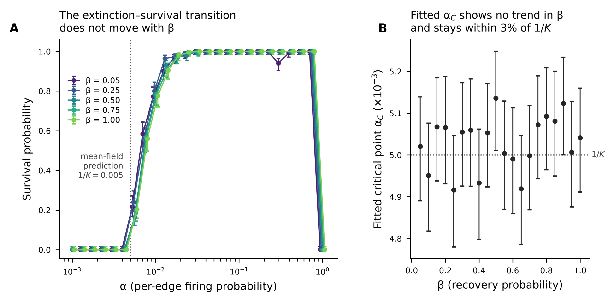
Sweeping α indeed produces the extinct–survived boundary that excitable-network theory predicts. Below a critical value α_C the cascades die out. Above it, the cascades self-sustain (Figure 2A). In reality, in cortical tissue, neuronal avalanches are often observed near this transition regime³⁷. No run survived at or below α = 4.2 × 10⁻³ (0 of 30,000 runs); survival first appeared at α = 5.6 × 10⁻³ (20.3% of 5,000 runs); a maximum-likelihood fit of the mean-field branching-process survival probability places the critical point at α_C = (5.03 ± 0.03) × 10⁻³ (95% confidence interval). The last fully-extinct grid value only bounds the critical point from below; the apparent 16% gap to the prediction reflects the grid spacing (0.125 decades). The fitted value agrees with theory: Kinouchi and Copelli²⁴ show such networks become critical when the branching ratio (here σ ≈αK) equals one, predicting α ≈ 1/K = 0.005 for K = 200, within 0.6% of our fitted α_C; Reyes²⁰ reports the same product form (rK constant at the transition) in small-world Greenberg–Hastings networks. Near-critical dynamics and rhythms can coexist: self-organized-critical neural models show noisy local dynamics driving avalanche statistics toward mean-field behavior³⁸ and scale-free avalanches coexisting with rhythms under oscillatory perturbation^39,40,41; the sampled regime permits oscillations. The boundary is essentially independent of β, as Larremore et al.⁴² predict: survival curves at five β coincide through the transition (Figure 2A), the critical point fitted at each of the twenty β values shows no trend, staying within 2.7% of 1/K (Figure 2B), and across all 500 (α, β) grid cells the rank correlation between survival and β is ρ = 0.01 (p = 0.82). Qian²² identified a bounded connection-probability window (roughly 0.004 to 0.034) for collective oscillations in excitable Erdős–Rényi networks; ours, P = K/N = 0.01, lies inside it (indicative only, derived for much smaller deterministic systems).

Spectral sharpness and genuine repetition can disagree

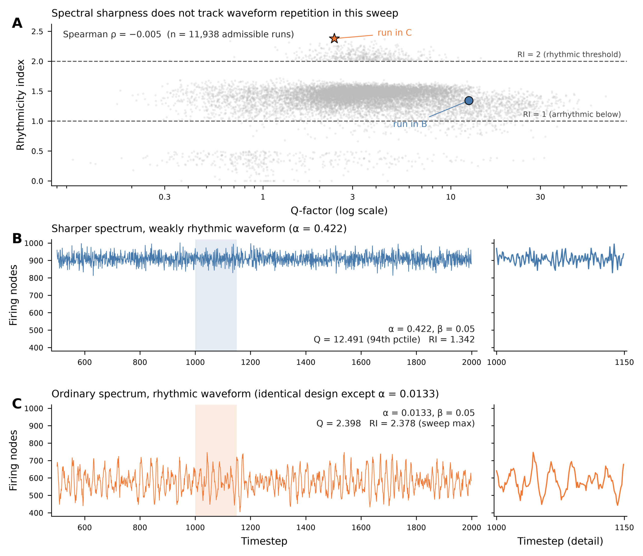
Figure 3A shows the joint distribution of the Q-factor and the rhythmicity index over the 11,938 surviving runs passing the admissibility floors (the floors exclude 70,262 surviving runs, predominantly short-period fast-flip dynamics — median period ≈ 3.4 timesteps, fewer points per cycle than the shape measure needs — whose share rises from 45% of survivors at β = 0.05 to 95% at β = 1.00). The two measures are uncorrelated, Spearman ρ = −0.005 (bootstrap 95% CI [−0.022, 0.014]). All 120 top-percentile-Q runs fall below the rhythmic threshold (RI < 2; median RI = 1.26) and 5% are arrhythmic.

The sweep’s largest Q, 66.8, is an extreme-value artifact: the estimator flags it resolution-limited (half-power width under 3 FFT bins), as it does 80% of top-percentile-Q runs; its components (c = 0.124, c̄ = 0.104, r = 0.501 at a period of 4.52 timesteps) fail both phase-consistency thresholds (only the shape term r clears its bar), and the period leaves fewer than the eight points per cycle the shape measure needs: inadmissible for scoring. Against 200 phase-randomised surrogate families (spectra preserved, waveform structure destroyed; 82,194 of the 82,200 survivors remained active at the final timestep and enter the surrogate test) and 200 AR(1)-matched families (matched mean, variance, lag-1 autocorrelation), the observed maximum lies inside the phase-randomised surrogate-maximum distribution (68.2 ± 4.7, range 60.6–82.4; one-sided p = 0.58) and below the entire AR(1) distribution (87.9 ± 3.3; p = 1.00).

Figures 3B and 3C contrast two runs identical in design except for α. At α = 0.422 (Figure 3B) the spectral peak is sharp (Q = 12.49, the 94th percentile of admissible runs, resolved across 6.8 FFT bins), yet RI = 1.342 (c = 0.229, c̄ = 0.190, r = 0.304), weakly rhythmic. At α = 0.0133 (Figure 3C) the spectrum is unremarkable (Q = 2.40, the 28th percentile) but the waveform repeats for 57.5 cycles at a period of 26.08 timesteps (26.1 samples per cycle): RI = 2.378 (c = 0.568, c̄ = 0.545, r = 0.551), the highest among all admissible runs — ranked by Q, B > C; the index reverses the order. Both traces are stationary in mean (linear drift −0.20% and −0.05%, both p > 0.45); amplitude variability, coefficient of variation 0.032 (B) versus 0.104 (C), runs against the index’s verdict. We did not match the amplitudes of the two runs by selection: the comparison run’s smaller relative amplitude, if anything, favors it, and both traces are drawn on a common y-range (Figure 3). The mechanism is the one this model class is known for: a slow refractory period stabilizes self-sustained dynamics into collective oscillations²¹: the exemplar and all 25 top admissible high-RI candidates lie at the sweep’s lowest recovery probability, β = 0.05.

The rhythmicity index transfers to human EEG (Berger effect)

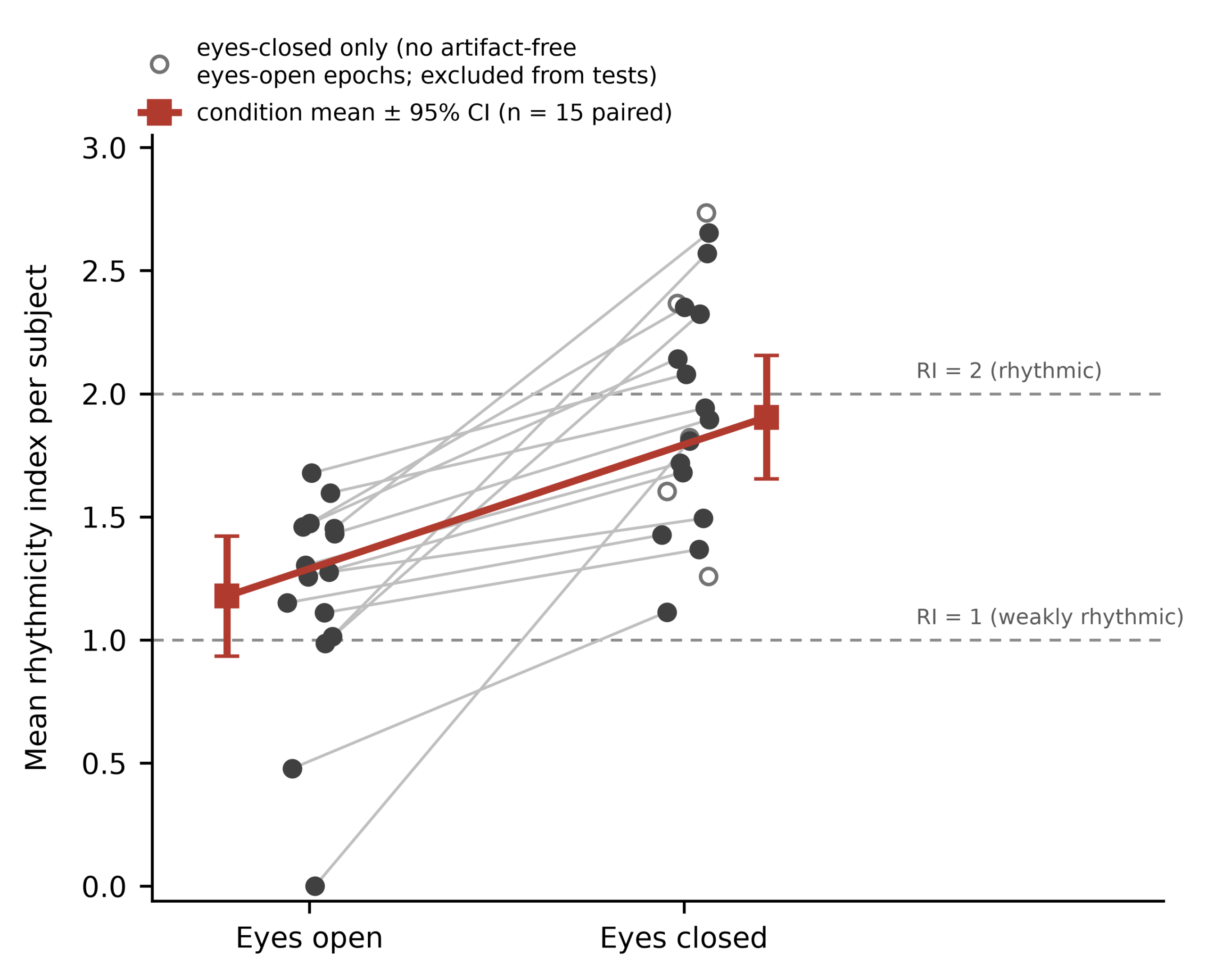
Applied to broadband-filtered EEG with each epoch’s dominant frequency estimated freely, the index recovers the Berger effect at the subject level: across the 15 subjects with artifact-free data in both conditions, the mean rhythmicity index rises from 1.178 with eyes open to 1.904 with eyes closed (SDs in Supporting Online Material, Table S6), a within-subject increase of 0.726 (95% CI 0.442 to 1.010; paired t(14) = 5.49, p = 8 × 10⁻⁵; d_z = 1.42), with all 15 subjects increasing (Figure 4). The estimated dominant frequency behaves as physiology predicts: eyes-closed median 10.2 Hz, 80% of admissible epochs peaking inside 8–13 Hz; eyes-open median 6.1 Hz, 24% in the alpha band: the pipeline finds alpha rather than being told where to look.

The original submission’s Cohen’s d = 1.08 pooled all 600 epochs as if independent; epochs within a subject are correlated, so subject-level statistics are reported throughout. Narrowband filtering, by contrast, manufactures rhythmicity: with the original 8–13 Hz filter the mean eyes-open index is 2.599 (above the rhythmic threshold on data where alpha is largely absent), filtering having imposed phase and shape regularity on in-band power; the condition difference survives (d_z = 0.76) but the absolute values are uninterpretable.

Per subject, 8 of 20 eyes-closed means reach the rhythmic band, 12 the weakly rhythmic band, none is arrhythmic (eyes-open: none rhythmic, 12 of 15 weakly rhythmic, 3 arrhythmic). The eyes-closed group mean of 1.904 sits just below the rhythmic boundary because alpha waxes and wanes across epochs, not because it is misclassified.

Identical epochs allow an honest baseline comparison (paired statistics, n = 15; Supporting Online Material, Table S6). Eyes-closed occipital alpha is a genuine narrowband oscillation, so every spectral quantity also separates the conditions: the Q-factor at d_z = 1.68, alpha-band log₁₀ power at 1.65, specparam alpha peak power at 1.65, and the shape term r alone at 1.65; the composite index’s d_z = 1.42 is not the largest effect size in the comparison; we do not claim otherwise.

The index is validated against an independent ground truth and a blinded visual rating

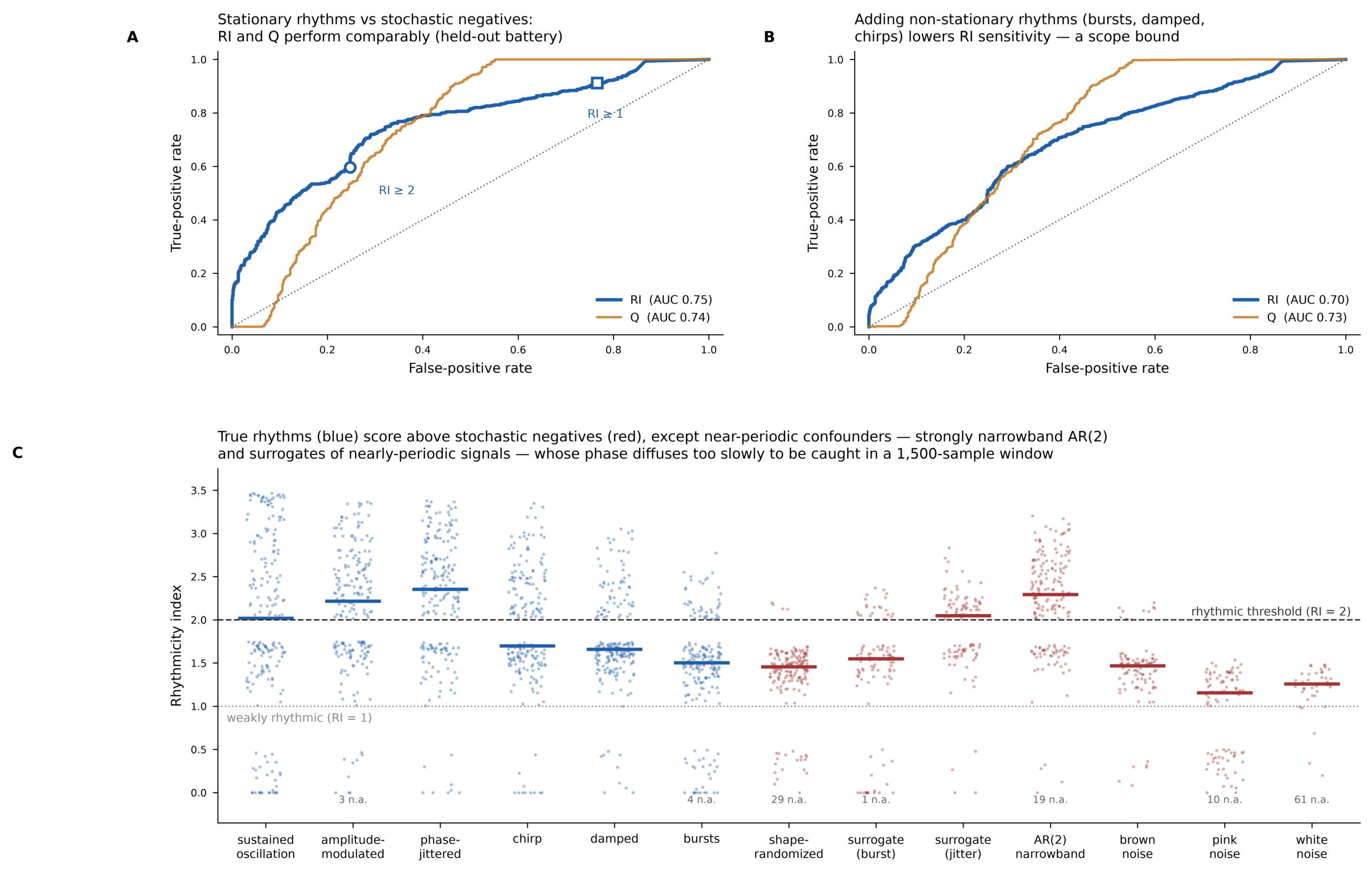
Sweep runs lack rhythmicity annotation besides the computed indices, so we curated a database of 2,146 synthetic signals with predetermined rhythmicity properties. Positive signal families represent a true repeating signal, increasingly corrupted (persistent, amplitude-modulated, jittery, bursty, damped and chirped oscillations) while negative signal families do not display a systematic repeating pattern (white, pink and brown noise; AR(2) band-limited noise; spectrum-matched surrogates of jittery and bursty rhythms; and randomized-signals preserving cycle time while changing the waveform for each cycle). All signals consist of 1,500 samples; we pre-define all constant parameters and grids, and all results use hold-out evaluation seeds (Table S2, family-wise results in the Supporting Online Material).

There are two separate sets of ground truth for the validation of our findings. In one case, a subset of stationary signals includes 500 positive signals (persistent, amplitude modulated and mild jittery rhythms) and compares to 900 negative signals (nonrepeating, no rhythmicity). For these signals, the index achieves an ROC area of 0.75 (Figure 5A, bootstrap 95% confidence interval 0.73–0.78) compared to Q’s of 0.74 (0.72–0.77). Using fixed threshold decisions, the sensitivity is 0.60 and specificity is 0.75 at the rhythmic threshold (RI ≥ 2), or sensitivity is 0.91 and specificity is 0.23 at the weakly-rhythmic threshold (RI ≥ 1). Adding nonstationary signal classes (bursty, damped oscillation and broad chirps), which brings the positive set to 1,196 rhythms, reduces the RI area value to 0.70 (compared to Q’s 0.73).

The index’s principal failure mode is strongly narrowband AR(2) noise: pooled over pole radii RI’s area is 0.53 (Q: 0.83), and at pole radius 0.99, 96% of instances cross RI ≥ 2, because a slowly drifting resonance is indistinguishable from a rhythm over the ~40 cycles a 1,500-sample window holds. Multiplying the record length by 4, to 6,000 samples, recovers the separation (area ≈ 0.7); hence the limit is on record length, not on how the index works. The phase-randomized surrogates of stationary rhythms are not used in calculating the ROC since they still have rhythmic structure (76% of them are above the threshold of RI = 2), as one would expect from a shape-sensitive metric; thus the effectiveness of the index needs to be judged against broadband surrogates instead of surrogates of the rhythms themselves.

To test the index visually, we conducted a complementary blinded analysis comparing the index against the visual appearance of the model’s own data. We plotted 36 admissible sweep runs (a 3 × 3 design of RI category by Q tercile) identically and had them rated blind for apparent rhythmicity by a vision-language model in three rounds (rater limitations in the Supporting Online Material). Ratings tracked RI (Spearman ρ = 0.46, p = 0.005) but not Q (ρ = −0.13, p = 0.44): the runs the spectral criterion ranks highest looked least rhythmic to the blinded rater (Supporting Online Material, Fig. S1 and Table S1).

Discussion

Our central finding is that the rhythmicity index can indicate genuine periodicity where spectral sharpness alone cannot. Across the 11,938 admissible runs of a 125,000-run sweep, spectral sharpness and measured rhythmicity were uncorrelated (ρ = −0.005), every top-percentile-Q run fell below the rhythmic threshold, and the sweep’s maximum Q was indistinguishable from the maxima of matched noise with no periodic structure. This demonstrates a recurring concern in the methods literature: a narrow spectral peak can arise from a dominant frequency band in noise without any repeating waveform^7,10,11,17. The remedy is time-domain verification, which the index operationalizes: requiring phase and shape consistency (Figure 1), it cannot be fooled by a signal satisfying only one (Figure 3).

Spectral parameterization, the current detection standard⁵, sharpens this point. Fitted to the same 82,200 surviving runs and all 600 EEG epochs, specparam’s peak power is a much better rhythmicity proxy than the raw Q-factor (ρ with RI = +0.53 versus −0.005), yet 50.8% of its top-percentile peak-power runs still fall below the rhythmic threshold: power above the aperiodic background cannot tell whether the waveform repeats. So RI is not an alternative to spectral parameterization, but a final time-domain verification step beyond spectral detection.

We make no assertion that this index is universally superior to the Q-factor, because the two coincide for a clean, narrowband oscillation; but since users do not know in advance what sort of signal they have in hand, an indicator which agrees with spectral sharpness when it is trustworthy, and deviates otherwise, is a valuable guardrail.

The best validation that this index captures physical reality rather than idiosyncrasies of the modeling system is its generalization to human EEG: using the identical code that scored the simulated data, we find the Berger effect in human data with a large effect size. The natural next test of generator-independence is to apply the index to more biophysically detailed models: Izhikevich networks, where rhythms and synchronization transitions depend on topology and synaptic type⁴³, and spiking Hodgkin–Huxley networks, where the character of the synchronization transition itself changes with topology and synaptic interaction⁴⁴, where limit-cycle ground truth is available from the model state.

Limitations

First, our model generator does not faithfully capture any neural tissue or network, but represents a minimal set of rules for excitability. Second, the bands designated at RI = 1 and RI = 2 are conventions; which band a signal falls into depends on the constants: as many as 16.3% of admissible runs change band if the thresholds are set to the extremes, and 22% to 85% of eyes-closed EEG epochs are classified as “rhythmic” across swept threshold settings (Supporting Online Material, Table S3); however, the relative orderings remain unchanged, and the EEG effect, the Q–RI decoupling, and the exemplar contrast persist across the tolerance intervals stated in the Methods. To provide a more relaxed test of our approach, in an auxiliary analysis of our model’s history, we used a relaxed screen (RI ≥ 1.5) rather than the strict cutoff (RI ≥ 2) that was otherwise used throughout; we chose this relaxed cutoff based on our observed rates of passing at the default screen, though the results in our paper did not include this auxiliary test. We provide the details here so that the claim that the constants were fixed before the EEG analysis stays checkable. Third, because AR(2) noise near its resonant pole mimics a genuine rhythm at these record lengths, distinguishing true rhythms from such noise is constrained by record length and becomes more accurate as the window grows (see The index is validated against an independent ground truth and a blinded visual rating); additionally, using entire records to score a signal makes short bursts, strongly damped oscillations and wide chirps score low by design. Fourth, narrow-band filters artificially impose regularity on the signal in the process of extracting a band — for example, band-filtering eyes-open EEG between 8 and 13 Hz pushes the mean index above the rhythmic threshold even though alpha is largely absent (see The rhythmicity index transfers to human EEG); therefore, the index should be applied to raw broadband signals, with the spectral peak estimated automatically from the data. Finally, relying on a single exemplar is risky. Our primary evidence comes from analyzing the entire distributions of scores for many signals, and our exemplar (Figure 3) serves more as an illustrative summary, rather than direct demonstration, of the performance of the metric.

Conclusions

Spectral sharpness alone does not establish that a signal genuinely repeats. A rhythmicity index requiring both phase and shape consistency recovers most genuinely periodic signals (sensitivity 0.91 at the weakly-rhythmic boundary on the stationary battery) and, developed entirely on simulated data, transfers to human EEG, recovering the Berger effect at large effect size. Where it matters whether a signal genuinely repeats, periodicity is best confirmed in the time domain rather than inferred from the sharpness of a spectral peak alone. The index is one simple way to do so (a safeguard against a key Q-factor failure mode, not a replacement), and the code applies to any evenly sampled series in one call (a few milliseconds per 1,500-sample trace). For each new input type, users should first check the data’s minimum requirements (eight samples per cycle and ten cycles per window); the decision thresholds may stay at their default values, but if users require carefully calibrated output categories, they should verify whether the band boundaries align with known ground truth and modify the threshold values as needed.

Data and Code Availability

All simulation and analysis code, including the rhythmicity-index implementation, is available at https://github.com/VRuikeLiu/rhythmicity-index (MIT-licensed). The EEG data are the publicly available EEG Motor Movement/Imagery Database (EEGMMIDB) from PhysioNet, https://physionet.org/content/eegmmidb/1.0.0/^33,34. The results tables, which contain the Q-factor and rhythmicity-index values for each of our 125,000 sweep runs, along with the example input signals that produce the illustrated results, have been uploaded to our repository so that readers can reproduce any of the presented figures without running the full set of simulations themselves.

Author Contributions

R.L. conceived the study, implemented the model and the rhythmicity index, ran the simulations and EEG analysis, and drafted the manuscript. A.M. supervised the project, advised on the model and its interpretation, and revised the manuscript.

Competing Interests

The authors declare no competing interests.

Acknowledgments

The author thanks his parents and sister for their company alongside the process of producing this paper. The author also thanks Dr. Katherine Alex from The Governor’s Academy for her attention and help on the project. Finally, the author wants to thank his friends at The Governor’s Academy for constantly motivating him to complete this project. A Generative AI tool (Claude, Anthropic) was used, under the author’s direction and with the author’s verification of every result, to help write and debug analysis code, run and check analyses, perform the visual audit as specified in the Supporting Online Material, and search the literature. The native add-in of ChatGPT by OpenAI inside Word was used for formatting purposes. They were, however, not used to draft, paraphrase, expand, or rewrite prose. The author takes full responsibility for the content.

Supplementary Information

References

1. S. P. Muscinelli, W. Gerstner, T. Schwalger. How single neuron properties shape chaotic dynamics and signal transmission in random neural networks. PLOS Computational Biology. Vol. 15, pg. e1007122, 2019, https://doi.org/10.1371/journal.pcbi.1007122. [↩] [↩]
2. A. Pérez-Cervera, B. Gutkin, P. J. Thomas, B. Lindner. A universal description of stochastic oscillators. Proceedings of the National Academy of Sciences. Vol. 120, pg. e2303222120, 2023, https://doi.org/10.1073/pnas.2303222120. [↩]
3. T. A. Whitten, A. M. Hughes, C. T. Dickson, J. B. Caplan. A better oscillation detection method robustly extracts EEG rhythms across brain state changes: the human alpha rhythm as a test case. NeuroImage. Vol. 54, pg. 860–874, 2011, https://doi.org/10.1016/j.neuroimage.2010.08.064. [↩]
4. J. Q. Kosciessa, T. H. Grandy, D. D. Garrett, M. Werkle-Bergner. Single-trial characterization of neural rhythms: potential and challenges. NeuroImage. Vol. 206, pg. 116331, 2020, https://doi.org/10.1016/j.neuroimage.2019.116331. [↩]
5. T. Donoghue, M. Haller, E. J. Peterson, P. Varma, P. Sebastian, R. Gao, T. Noto, A. H. Lara, J. D. Wallis, R. T. Knight, A. Shestyuk, B. Voytek. Parameterizing neural power spectra into periodic and aperiodic components. Nature Neuroscience. Vol. 23, pg. 1655–1665, 2020, https://doi.org/10.1038/s41593-020-00744-x. [↩] [↩] [↩]
6. M. Gerster, G. Waterstraat, V. Litvak, K. Lehnertz, A. Schnitzler, E. Florin, G. Curio, V. Nikulin. Separating neural oscillations from aperiodic 1/f activity: challenges and recommendations. Neuroinformatics. Vol. 20, pg. 991–1012, 2022, https://doi.org/10.1007/s12021-022-09581-8. [↩]
7. S. R. Jones. When brain rhythms aren’t ‘rhythmic’: implication for their mechanisms and meaning. Current Opinion in Neurobiology. Vol. 40, pg. 72–80, 2016, https://doi.org/10.1016/j.conb.2016.06.010. [↩] [↩]
8. M. Lundqvist, J. Rose, P. Herman, S. L. Brincat, T. J. Buschman, E. K. Miller. Gamma and beta bursts underlie working memory. Neuron. Vol. 90, pg. 152–164, 2016, https://doi.org/10.1016/j.neuron.2016.02.028. [↩]
9. H. Shin, R. Law, S. Tsutsui, C. I. Moore, S. R. Jones. The rate of transient beta frequency events predicts behavior across tasks and species. eLife. Vol. 6, pg. e29086, 2017, https://doi.org/10.7554/eLife.29086. [↩]
10. S. R. Cole, B. Voytek. Brain oscillations and the importance of waveform shape. Trends in Cognitive Sciences. Vol. 21, pg. 137–149, 2017, https://doi.org/10.1016/j.tics.2016.12.008. [↩] [↩]
11. S. R. Cole, B. Voytek. Cycle-by-cycle analysis of neural oscillations. Journal of Neurophysiology. Vol. 122, pg. 849–861, 2019, https://doi.org/10.1152/jn.00273.2019. [↩] [↩] [↩]
12. S. R. Cole, R. van der Meij, E. J. Peterson, C. de Hemptinne, P. A. Starr, B. Voytek. Nonsinusoidal beta oscillations reflect cortical pathophysiology in Parkinson’s disease. Journal of Neuroscience. Vol. 37, pg. 4830–4840, 2017, https://doi.org/10.1523/JNEUROSCI.2208-16.2017. [↩]
13. N. Schaworonkow, V. V. Nikulin. Spatial neuronal synchronization and the waveform of oscillations: implications for EEG and MEG. PLOS Computational Biology. Vol. 15, pg. e1007055, 2019, https://doi.org/10.1371/journal.pcbi.1007055. [↩]
14. A. J. Quinn, V. Lopes-dos-Santos, N. Huang, W.-K. Liang, C.-H. Juan, J.-R. Yeh, A. C. Nobre, D. Dupret, M. W. Woolrich. Within-cycle instantaneous frequency profiles report oscillatory waveform dynamics. Journal of Neurophysiology. Vol. 126, pg. 1190–1208, 2021, https://doi.org/10.1152/jn.00201.2021. [↩]
15. N. Schaworonkow. Overcoming harmonic hurdles: genuine beta-band rhythms vs. contributions of alpha-band waveform shape. Imaging Neuroscience. Vol. 1, pg. 1–8, 2023, https://doi.org/10.1162/imag_a_00018. [↩]
16. S. Bartz, F. S. Avarvand, G. Leicht, G. Nolte. Analyzing the waveshape of brain oscillations with bicoherence. NeuroImage. Vol. 188, pg. 145–160, 2019, https://doi.org/10.1016/j.neuroimage.2018.11.045. [↩]
17. A. M. M. Fransen, F. van Ede, E. Maris. Identifying neuronal oscillations using rhythmicity. NeuroImage. Vol. 118, pg. 256–267, 2015, https://doi.org/10.1016/j.neuroimage.2015.06.003. [↩] [↩] [↩]
18. J. M. Greenberg, S. P. Hastings. Spatial patterns for discrete models of diffusion in excitable media. SIAM Journal on Applied Mathematics. Vol. 34, pg. 515–523, 1978, https://doi.org/10.1137/0134040. [↩] [↩]
19. G. B. Ermentrout, L. Edelstein-Keshet. Cellular automata approaches to biological modeling. Journal of Theoretical Biology. Vol. 160, pg. 97–133, 1993, https://doi.org/10.1006/jtbi.1993.1007. [↩]
20. L. I. Reyes. Greenberg–Hastings dynamics on a small-world network: the effect of disorder on the collective extinct–active transition. arXiv:1505.00182v6, 2017, https://arxiv.org/abs/1505.00182. [↩] [↩]
21. S. A. Moosavi, A. Montakhab, A. Valizadeh. Refractory period in network models of excitable nodes: self-sustaining stable dynamics, extended scaling region and oscillatory behavior. Scientific Reports. Vol. 7, pg. 7107, 2017, https://doi.org/10.1038/s41598-017-07135-6. [↩] [↩]
22. Y. Qian. Emergence of self-sustained oscillations in excitable Erdős–Rényi random networks. Physical Review E. Vol. 90, pg. 032807, 2014, https://doi.org/10.1103/PhysRevE.90.032807. [↩] [↩]
23. L. Brochini, A. de Andrade Costa, M. Abadi, A. C. Roque, J. Stolfi, O. Kinouchi. Phase transitions and self-organized criticality in networks of stochastic spiking neurons. Scientific Reports. Vol. 6, pg. 35831, 2016, https://doi.org/10.1038/srep35831. [↩]
24. O. Kinouchi, M. Copelli. Optimal dynamical range of excitable networks at criticality. Nature Physics. Vol. 2, pg. 348–351, 2006, https://doi.org/10.1038/nphys289. [↩] [↩] [↩]
25. P. Erdős, A. Rényi. On the evolution of random graphs. Publications of the Mathematical Institute of the Hungarian Academy of Sciences. Vol. 5, pg. 17–61, 1960. [↩]
26. M. E. J. Newman. Networks: an introduction. Oxford University Press, 2010, https://doi.org/10.1093/acprof:oso/9780199206650.001.0001. [↩]
27. P. Welch. The use of fast Fourier transform for the estimation of power spectra: a method based on time averaging over short, modified periodograms. IEEE Transactions on Audio and Electroacoustics. Vol. 15, pg. 70–73, 1967, https://doi.org/10.1109/TAU.1967.1161901. [↩]
28. P. Virtanen, R. Gommers, T. E. Oliphant, M. Haberland, T. Reddy, D. Cournapeau, E. Burovski, P. Peterson, W. Weckesser, J. Bright, S. J. van der Walt, M. Brett, J. Wilson, K. J. Millman, N. Mayorov, A. R. J. Nelson, E. Jones, R. Kern, E. Larson, C. J. Carey, İ. Polat, Y. Feng, E. W. Moore, J. VanderPlas, D. Laxalde, J. Perktold, R. Cimrman, I. Henriksen, E. A. Quintero, C. R. Harris, A. M. Archibald, A. H. Ribeiro, F. Pedregosa, P. van Mulbregt, SciPy 1.0 Contributors. SciPy 1.0: fundamental algorithms for scientific computing in Python. Nature Methods. Vol. 17, pg. 261–272, 2020, https://doi.org/10.1038/s41592-019-0686-2. [↩]
29. A. M. M. Fransen, G. Dimitriadis, F. van Ede, E. Maris. Distinct α- and β-band rhythms over rat somatosensory cortex with similar properties as in humans. Journal of Neurophysiology. Vol. 115, pg. 3030–3044, 2016, https://doi.org/10.1152/jn.00507.2015. [↩]
30. H. Berger. Über das Elektrenkephalogramm des Menschen. Archiv für Psychiatrie und Nervenkrankheiten. Vol. 87, pg. 527–570, 1929, https://doi.org/10.1007/BF01797193. [↩]
31. R. J. Barry, F. M. De Blasio. EEG differences between eyes-closed and eyes-open resting remain in healthy ageing. Biological Psychology. Vol. 129, pg. 293–304, 2017, https://doi.org/10.1016/j.biopsycho.2017.09.010. [↩]
32. W. Hohaia, B. W. Saurels, A. Johnston, K. Yarrow, D. H. Arnold. Occipital alpha-band brain waves when the eyes are closed are shaped by ongoing visual processes. Scientific Reports. Vol. 12, pg. 1194, 2022, https://doi.org/10.1038/s41598-022-05289-6. [↩]
33. A. L. Goldberger, L. A. N. Amaral, L. Glass, J. M. Hausdorff, P. C. Ivanov, R. G. Mark, J. E. Mietus, G. B. Moody, C. K. Peng, H. E. Stanley. PhysioBank, PhysioToolkit, and PhysioNet: components of a new research resource for complex physiologic signals. Circulation. Vol. 101, pg. e215–e220, 2000, https://doi.org/10.1161/01.CIR.101.23.e215. [↩] [↩]
34. G. Schalk, D. J. McFarland, T. Hinterberger, N. Birbaumer, J. R. Wolpaw. BCI2000: a general-purpose brain–computer interface (BCI) system. IEEE Transactions on Biomedical Engineering. Vol. 51, pg. 1034–1043, 2004, https://doi.org/10.1109/TBME.2004.827072. [↩] [↩]
35. A. Gramfort, M. Luessi, E. Larson, D. A. Engemann, D. Strohmeier, C. Brodbeck, R. Goj, M. Jas, T. Brooks, L. Parkkonen, M. Hämäläinen. MEG and EEG data analysis with MNE-Python. Frontiers in Neuroscience. Vol. 7, pg. 267, 2013, https://doi.org/10.3389/fnins.2013.00267. [↩]
36. M. Jas, D. A. Engemann, Y. Bekhti, F. Raimondo, A. Gramfort. Autoreject: automated artifact rejection for MEG and EEG data. NeuroImage. Vol. 159, pg. 417–429, 2017, https://doi.org/10.1016/j.neuroimage.2017.06.030. [↩]
37. J. M. Beggs, D. Plenz. Neuronal avalanches in neocortical circuits. Journal of Neuroscience. Vol. 23, pg. 11167–11177, 2003, https://doi.org/10.1523/JNEUROSCI.23-35-11167.2003. [↩]
38. S. A. Moosavi, A. Montakhab. Mean-field behavior as a result of noisy local dynamics in self-organized criticality: neuroscience implications. Physical Review E. Vol. 89, pg. 052139, 2014, https://doi.org/10.1103/PhysRevE.89.052139. [↩]
39. S. A. Moosavi, A. Montakhab, A. Valizadeh. Coexistence of scale-invariant and rhythmic behavior in self-organized criticality. Physical Review E. Vol. 98, pg. 022304, 2018, https://doi.org/10.1103/PhysRevE.98.022304. [↩]
40. L. Dalla Porta, M. Copelli. Modeling neuronal avalanches and long-range temporal correlations at the emergence of collective oscillations: continuously varying exponents mimic M/EEG results. PLOS Computational Biology. Vol. 15, pg. e1006924, 2019, https://doi.org/10.1371/journal.pcbi.1006924. [↩]
41. S. di Santo, P. Villegas, R. Burioni, M. A. Muñoz. Landau–Ginzburg theory of cortex dynamics: scale-free avalanches emerge at the edge of synchronization. Proceedings of the National Academy of Sciences. Vol. 115, pg. E1356–E1365, 2018, https://doi.org/10.1073/pnas.1712989115. [↩]
42. D. B. Larremore, W. L. Shew, E. Ott, J. G. Restrepo. Effects of network topology, transmission delays, and refractoriness on the response of coupled excitable systems to a stochastic stimulus. Chaos. Vol. 21, pg. 025117, 2011, https://doi.org/10.1063/1.3600760. [↩]
43. M. Khoshkhou, A. Montakhab. Beta-rhythm oscillations and synchronization transition in network models of Izhikevich neurons: effect of topology and synaptic type. Frontiers in Computational Neuroscience. Vol. 12, pg. 59, 2018, https://doi.org/10.3389/fncom.2018.00059. [↩]
44. M. Khoshkhou, A. Montakhab. Explosive, continuous and frustrated synchronization transition in spiking Hodgkin–Huxley neural networks: the role of topology and synaptic interaction. Physica D: Nonlinear Phenomena. Vol. 405, pg. 132399, 2020, https://doi.org/10.1016/j.physd.2020.132399. [↩]