Probing Frozen Visual Representations for Safety-Relevant Structure in MiniGrid LavaGap Navigation: A Geometric Comparison of DINOv3 and ResNet-50 

Abstract

Background/Objective: Embodied AI systems must act safely in complex environments. Self-supervised learning (SSL) produces rich visual representations from unlabeled data and may capture safety-relevant structure. We ask whether two frozen encoders, the self-supervised DINOv3 and an ImageNet-supervised ResNet-50, encode such structure in grid-navigation states without safety-specific supervision.
Methods: In MiniGrid LavaGapS7 we labeled 5,000 states safe, near-boundary, or unsafe by the agent’s position. Because the environment admits only 732 distinct states, we deduplicated and withheld three of the 15 layouts, then fitted SVM probes and a label-free One-Class SVM on training data only. Two controls, raw 32×32 pixels and a randomly initialized ResNet-50, used the identical pipeline.
Results: An untrained network detected lava nearly as well as the pre-trained encoders, so the unsafe class is recoverable without any learned representation. On safe versus near-boundary the encoders diverged sharply: on withheld layouts DINOv3 identified all 18 held-out safe states (balanced accuracy 1.000) and a label-fine-tuned ResNet-50 identified 16, whereas the frozen ImageNet ResNet-50 identified 1 (balanced accuracy 0.528, despite 0.974 raw accuracy). The label-free detector reproduced this ordering (AUROC 0.975 versus 0.750), as did silhouette scores (0.111 versus 0.017).
Conclusions: Frozen self-supervised features expose a spatial relation, agent-to-boundary proximity, recoverable neither from raw pixels nor a random network nor ImageNet-supervised features, and it transfers to unseen layouts without safety supervision. This is not abstract safety understanding, since the labels remain a static function of visible geometry, but it is a concrete representational difference that a leaky evaluation had hidden.

Keywords: self-supervised learning; embodied AI; safety; representation geometry; anomaly detection

Introduction

Embodied AI refers to AI systems situated in physical bodies or simulated environments, capable of perceiving, making decisions, acting, and learning in real-world environments^1,2. These systems have shown growing potential in robotics, autonomous driving, surgical assistance, and healthcare, where agents must operate in complex, dynamic, and unpredictable environments^1,2,3,4. In autonomous driving, end-to-end systems must interpret complex traffic scenes, anticipate the behavior of other road users, and plan driving actions⁵. Embodied AI has also contributed to medicine: the STAR system has demonstrated potential in autonomous soft-tissue surgery, while rehabilitation robots interact with patients and adapt therapy through feedback^3,4.

However, developing reliable embodied agents typically requires large amounts of labeled data covering diverse real-world situations, which makes the process time-consuming and costly^6,7,8,9. Self-supervised learning (SSL) offers a practical solution by enabling models to learn from unlabeled data while automatically generating their own training signals. These signals are created through objectives such as contrastive learning, masked reconstruction, and predictive world modeling, and have been shown to rival or exceed conventional supervised training: masked autoencoders (MAE), for example, reach 87.8% accuracy on ImageNet-1K¹⁰.

A prominent challenge that still limits the deployment of these systems is safety. Unlike conventional visual-recognition tasks, safety in embodied agents is difficult to define because failures are not determined solely by what is visible in a single frame. Instead, unsafe outcomes can emerge from interactions among perception, planning, action, and environmental dynamics. An agent may avoid an immediate collision yet still produce unsafe behavior, such as dropping an object, entering a restricted area, obstructing a path, or creating a delayed hazard^11,12,13,14. Safety often depends on the agent’s proximity to hazards and its upcoming actions, not merely on whether danger is currently occurring, which makes safety a contextual, trajectory-level property rather than a simple categorical label. In this study we deliberately operationalize a simpler, static proxy for this property, position-based proximity to hazards, and we return to the gap between the proxy and the full trajectory-level notion of safety in the Methods and Discussion.

Self-supervised learning may be well suited to this problem because SSL models are trained to organize visual inputs into semantically meaningful representations without explicit task labels. In principle, such representations may capture intermediate or ambiguous states, including near-boundary cases that are neither clearly safe nor clearly unsafe. It remains unclear, however, whether SSL representations are inherently better suited for safety-relevant state discrimination than representations learned through standard supervised training. A single pair of encoders cannot settle that general question, because publicly available checkpoints differ in architecture, pre-training data, and training objective simultaneously; this study therefore compares two specific, widely used encoders and frames its conclusions accordingly.

This study asks whether the frozen representations of two pre-trained encoders, the self-supervised DINOv3¹⁵ and an ImageNet-supervised ResNet-50¹⁶, encode safety-relevant structure in grid-navigation states without explicit safety supervision. Specifically, we ask: (1) Can these frozen representations distinguish safe, near-boundary, and unsafe navigation states using only a lightweight SVM probe, on layouts withheld from training, and beyond what trivial features (raw pixels, a randomly initialized network) already achieve? (2) Do the two encoders, which differ in architecture, pre-training data, and training objective, differ in how well and how they separate these states, and how do they compare with a ResNet-50 fine-tuned on the labels themselves? (3) Are the three classes arranged in feature space as a binary split (normal versus anomalous) or as a graded continuum, as measured by centroid and k-nearest-neighbor distances to the safe reference distribution?

Related Work

Understanding how self-supervised learning can support safety-critical applications in embodied AI first requires understanding the training methodologies underlying these approaches, which can be grouped into a few broad families¹⁷.

The deep metric learning family

The deep metric learning family trains encoders to organize embeddings so that visually similar images lie close together in feature space while dissimilar images are pushed apart¹⁷. These relationships are generated automatically: two augmented views of the same image form a positive pair, while views of different images serve as negatives¹⁷. SimCLR exemplifies this principle through contrastive loss that trains the model to recognize that two views of the same image belong together¹⁸. Later methods refine the idea: MeanShift removes the need for explicit negatives by moving each embedding toward the average of its nearest neighbors; NNCLR treats an image’s nearest neighbors, not only its augmentations, as positives to learn richer relationships; and SCL adds a rotation-prediction task to improve generalization when few labels are available^17,19,20,21. In practice, these methods have been applied to face verification, person re-identification, clustering, and fine-grained image retrieval¹⁷.

The self-distillation family

The self-distillation family trains a student network to match the output of a teacher network, usually a slowly updated version of the same model. The teacher provides stable targets, allowing the student to learn consistent representations from different views without negative pairs or an external pre-trained teacher¹⁷. BYOL shows that this design alone is enough to avoid collapse, the failure mode in which a model maps many different images to nearly identical representations, by having an online network predict the output of a target network whose weights are a moving average of the online ones²². DINO applies a similar idea to Vision Transformers, training a student to match a momentum teacher. Its features were found to capture object boundaries without any segmentation labels²³. DINOv3 scales this self-distillation recipe to a much larger unlabeled corpus (LVD-1689M) and adds mechanisms that stabilize dense features, producing frozen representations that transfer broadly; it is the self-supervised encoder probed in this study¹⁵. Self-distillation has produced transferable representations supporting object discovery, semantic segmentation, retrieval, robustness, and model compression¹⁷.

Joint-embedding and predictive architectures

Joint-embedding and predictive architectures learn by predicting missing or future information in a latent representation space rather than reconstructing every detail of the input. A model can predict the representation of a hidden image region, a future video frame, or a future environmental state¹⁷. PlaNet is an early application of this principle to control, learning to plan by rolling out predicted latent states instead of full images²⁴. V-JEPA extends the idea to video, predicting the latent representation of masked regions instead of pixels, and DINO-WM freezes a pre-trained DINOv2 encoder and predicts how its features change after different actions, letting an agent plan directly in that frozen latent space^17,25,26. In embodied AI, such predictive representations can serve as latent world models that link perception, prediction, decision-making, and action selection without manual annotation¹⁷.

A fourth family: masked reconstruction

A fourth, related family relies on masked reconstruction rather than latent prediction. MAE masks random patches of an image and trains an encoder-decoder to reconstruct the missing pixels directly¹⁰. Because its supervisory signal lives in pixel space rather than feature space, MAE is best treated as separate from JEPA-style architectures, even though both rely on a masking objective.

Self-supervised learning in embodied AI

The ability to learn from large-scale unlabeled data makes SSL well suited to embodied systems. Pre-trained representations can serve as visual encoders that turn pixels into useful features, whether trained with label supervision, as with ViT²⁷, with natural-language supervision, as with CLIP²⁸, or entirely without labels, as with the self-supervised methods above; they can also act as latent state spaces that compress the environment^29,30, or as world models that perceive, predict, and plan³¹. For example, R3M uses features learned from large collections of human videos as a fixed perception module for robot manipulation³², while MVP trains a visual encoder on masked images, keeps it fixed, and combines its features with proprioceptive information to support motor-control policies³³. DINO-WM goes beyond perception, using frozen DINO-family features as the latent space of a world model and predicting how those features change after actions so the agent can compare and plan action sequences²⁶.

Safety in embodied AI

Yet, one of the most critical requirements for real-world adoption remains under-explored: safety. There is a general lack of safety evaluations for SSL methods integrated into embodied systems, partly because safety is hard to define and measure. A robot may avoid collisions yet still produce an unsafe outcome, such as dropping an object^11,12. Agents must also act in interactive, unpredictable environments shaped by context, the downstream consequences of actions, and situations that are rare or absent from the training data¹². Because they operate in the open world, guaranteeing safety and testing every possible outcome is difficult¹².

The ASIMOV benchmark reflects this difficulty: it evaluates the semantic safety of robot behavior by pairing automatically generated images of undesirable outcomes with a high-level “robot constitution” that specifies how a robot should behave³⁴. Once safety is understood as more than collision avoidance, we identify three gaps in current research, which we term a calibration gap, a guarantee gap, and an evaluation gap; this three-part framing is our own organization of themes in the literature rather than an established taxonomy.

The first gap concerns calibration. Modern neural networks are often poorly calibrated, meaning their confidence scores do not reflect the probability that their predictions are correct³⁵. A deployed model should not only be accurate but also signal when it may be wrong, because embodied agents can perform well on data resembling their training distribution yet fail in open-world or safety-critical settings. UNISafe and FAIL-Detect address this by detecting out-of-distribution (OOD) situations and identifying failures during execution^13,14.

The second gap involves safety guarantees. Learned representations must have specific structural properties before they can support reliable safety boundaries. LatentCBF argues that existing latent filters may switch abruptly between a normal task policy and a separate safety policy, hurting task performance, and instead proposes a smoother control-barrier-function (CBF) filter trained with gradient penalties and data from both policies³⁶. Similarly, the Latent Policy Barrier (LPB) treats the latent representations of expert demonstrations as an implicit barrier separating safe in-distribution states from unsafe out-of-distribution states. Its reliability therefore depends on the quality of the demonstrations and the learned embedding space³⁷.

The third gap is evaluation: most studies test models on in-distribution benchmarks rather than open-world deployment settings.

Methodologically, our approach belongs to an established lineage that the safety literature above does not usually reference. Probing frozen representations with lightweight classifiers goes back to linear classifier probes³⁸, and using nearest-neighbor distances on deep features for out-of-distribution detection was analyzed systematically by Sun et al.³⁹ We adopt the same tools (frozen features, light probes, and kNN distances) and apply them to position-derived safety labels in a navigation environment.

These works motivate our paper, which aims to address the evaluation gap by examining how safety-related categories are organized in a controlled navigation environment. Existing approaches largely treat safety as a fixed supervised classification problem or build explicit boundaries from labeled demonstrations, leaving open whether frozen pre-trained representations already encode safety-relevant structure on their own. To investigate this, we test whether frozen self-supervised and supervised representations can separate safe, near-boundary, and unsafe states in a grid-navigation environment without any safety-specific training. Because such environments are small and deterministic, we treat the evaluation protocol itself as part of the object of study: we quantify how many distinct states exist, withhold entire layouts, and measure what trivial features already achieve, so that any residual difference between encoders can be attributed to the representations rather than to the split.

Methods

Research design and objectives

Our experiment investigates whether the visual features of a frozen self-supervised encoder (DINOv3) can distinguish safe states from near-boundary and unsafe states, compared to the visual features of a frozen supervised encoder (ResNet-50). Concretely, we test whether the native visual representations produced by the two frozen backbones can separate safety states, in a way that can be detected through distance-based geometry and lightweight SVM probes as the agent approaches a safety boundary in a grid-navigation task. Because the two encoders differ in architecture (ViT versus CNN), pre-training data (LVD-1689M versus ImageNet-1K), and training objective (self-distillation versus supervised classification), any difference we observe between them cannot be attributed to any one of these factors; the study is a comparison of two specific encoders, not a controlled test of self-supervision versus supervision.

Dataset and label generation

We conduct our experiment in MiniGrid, a lightweight 2D environment containing walls, lava cells, empty areas, and a goal tile that the agent must reach without stepping into lava⁴⁰. We use the LavaGap configuration (environment ID MiniGrid-LavaGapS7-v0, a 7×7 grid including the surrounding walls), in which the agent starts in the top-left corner and the goal tile lies in the bottom-right corner, on opposite sides of a vertical lava strip containing one narrow passage. The environment fixes the start and goal positions and randomizes only the gap: the lava column can occupy one of 3 positions and the gap one of 5 rows, so exactly 15 distinct layouts exist. A new layout is drawn at every episode reset, so the collected data span multiple layouts within each seed run.

Within this setup, the agent follows a random navigation policy, selecting one of three actions at each step with equal probability: turn left, turn right, or move forward. We log 5,000 timesteps in total, split approximately equally across three random-seed initializations (seeds 1, 2, and 3; 1,667/1,667/1,666 steps). At each step we log a unique state identifier, an RGB image of the current environment state, and agent metadata (row and column coordinates, direction, action, reward, episode number, safety label, distance to the nearest boundary, and termination flags). Episodes end when the agent reaches the goal, steps into lava, or hits the environment’s time limit, after which the environment is reset with a newly drawn layout. The 5,000 steps span 132 episodes (mean length 37.9 steps, median 28, range 1-196): 123 ended in lava, 5 reached the goal, and the remainder were truncated or still in progress when a seed’s step budget was exhausted.

Observations are full-grid renders, not the agent’s partial egocentric view: each state is rendered as a 224×224×3 RGB image (7 tiles × 32 pixels per tile) using the environment’s rgb_array renderer, which includes MiniGrid’s default field-of-view highlighting (the tiles visible to the agent are rendered lighter). Images are saved as PNG files without further processing.

For each timestep we also record a safety state, designed to capture cases that are ambiguous to the backbones and to emulate real-world safety tasks in which an agent’s position or action is not always clearly defined. We compute safety from the agent’s position using three mutually exclusive labels, applied in order of precedence: (1) unsafe, if the agent is on top of a lava cell (this check is applied first); (2) near-boundary, if the agent is not on lava and lies one grid step or less from the nearest wall or lava cell; and (3) safe, if the agent is more than one grid step from every wall and lava cell. Because unsafe takes precedence over the distance rule, the three labels partition the state space. The class is named “interior” in our data-collection code and in the figure legends; the text uses “safe” throughout.

Because stepping into lava terminates the episode, on-lava frames are the terminal frames of failed episodes: the state reached by the terminating action is rendered and logged before the environment is reset, so each unsafe frame is the final frame of its episode.

We measure distance with the Manhattan metric because the agent moves in 4-connected grid steps, so Manhattan distance equals the number of forward moves separating two cells and matches the environment’s action space⁴¹. Two properties of this labeling deserve emphasis. First, it merges wall proximity and lava proximity into a single near-boundary class even though the two hazards differ in consequence: walking into a wall merely fails the move, while walking into lava ends the episode. We merge them because both delimit the traversable region and because separating them creates classes too small for stable probing at our dataset size; of the 4,469 near-boundary states, 1,342 lie within one step of a lava cell while 3,127 are near-boundary through wall adjacency alone, so the class is dominated by wall proximity. Second, the label is a static, position-based proxy: it ignores orientation, the planned action, and the time horizon, so a state beside lava while facing away receives the same label as one facing into it. We use this proxy deliberately, as a necessary precondition: if frozen features cannot separate even position-defined proximity categories, they cannot support richer action-conditioned safety notions. The Discussion returns to what the proxy does and does not license us to conclude.

The environment’s small state space has a consequence that shapes the entire evaluation: with 15 layouts, roughly 20 reachable non-lava cells, and 4 orientations, only on the order of a thousand distinct (layout, position, orientation) states exist, so a dataset of 5,000 timesteps necessarily contains many exact duplicates, and consecutive frames from the same episode are strongly correlated. Any random timestep-level train/test split therefore places copies of the same visual state on both sides of the split. Duplication is quantified exactly in the Results, and every evaluation reported in this paper is computed on deduplicated data under the episode- and layout-grouped protocol described below.

Feature extraction

Embeddings, fixed-length numerical vectors representing each image in a high-dimensional feature space, were extracted from two frozen, pre-trained backbones. Neither frozen backbone was fine-tuned on the MiniGrid safety labels. DINOv3 is a self-supervised vision transformer trained on large-scale unlabeled images through self-distillation¹⁵. We used the ViT-B/16 checkpoint facebook/dinov3-vitb16-pretrain-lvd1689m via the Hugging Face Transformers image-feature-extraction pipeline with pooling enabled (pool=True), which returns the model’s pooled global image representation, producing a 768-dimensional vector per image. Images were preprocessed by the checkpoint’s default processor (DINOv3ViTImageProcessorFast): bilinear resize to 224×224 with no center crop, rescaling by 1/255, and normalization with the ImageNet statistics mean (0.485, 0.456, 0.406) and standard deviation (0.229, 0.224, 0.225). Because our renders are already 224×224, the resize is an identity operation. ResNet-50 is a supervised convolutional neural network pre-trained on the ImageNet-1K classification task using explicit category labels¹⁶. We used the Torchvision implementation with its default pre-trained weights (ResNet50_Weights.DEFAULT)⁴², removed the final classification layer by replacing it with the identity, and extracted the penultimate global-average-pooled representation, producing a 2,048-dimensional vector per image. Preprocessing used the transform bundled with those weights (resizing, center-cropping to 224×224, and ImageNet-statistics normalization). The resulting embeddings were stored with their state identifiers and used, without any normalization or dimensionality reduction, as input to the geometric, classification, and visualization analyses.

Geometric analysis

To examine how the three safety categories are organized in each feature space, we treat the safe states as the reference distribution, which is the set of states considered normal and non-dangerous, and quantify organization with two distance-based measures.

First, we compute the safe centroid (the average embedding of all safe states) and measure the Euclidean distance from every state’s raw, unnormalized embedding to this centroid. A smaller distance indicates the state lies closer to the average safe representation, while a larger distance means greater deviation.

Second, we compute the average Euclidean distance from each state to its five nearest safe embeddings using k-nearest neighbors (kNN, k = 5)⁴³. Unlike the centroid, which collapses the safe set into a single point, kNN compares each state with actual safe examples. Two implementation details matter for interpreting the safe-class numbers. In our original analysis the reference set contained all safe states and the query was not excluded from it, so when a safe state was scored its own embedding participated as one of its neighbors and contributed a zero distance; because the dataset also contains exact duplicate states, a state’s neighbors could additionally be identical copies of itself from other timesteps. Both effects deflate the safe-class mean kNN distance. All geometric results reported below therefore come from a corrected protocol computed on the 732 unique states, in which the reference set contains only unique safe embeddings and the self-match is excluded for safe queries (k + 1 neighbors requested, first dropped). Comparing these distances across the safe, near-boundary, and unsafe labels indicates whether the proximity categories are geometrically organized: if a backbone encodes such structure, near-boundary and unsafe states should generally appear farther from the safe reference than safe states do.

Anomaly detection

To test whether dangerous states can be detected without training on unsafe labels, we trained a One-Class SVM, an anomaly detector that learns only the majority “normal” group⁴⁴. The identical protocol was applied to all three feature extractors so that the anomaly-detection experiment supports the same comparison as the probes. Features were standardized with a scaler fitted only on training safe-state embeddings and applied unchanged to the other classes. The detector used an RBF kernel with nu = 0.1 and gamma = “scale”, and was fitted exclusively on the deduplicated safe states of the outer training partition defined below. It was then applied to the held-out states, assigning each an anomaly score (the negated decision function, so that higher scores mean less similar to the safe set). We evaluated anomaly-detection performance with AUROC for safe versus near-boundary states and safe versus unsafe states, where 0.5 represents random ranking and 1.0 represents perfect separation. Because no evaluated state was used to fit the detector, these values are held out by construction.

Separately, we evaluated pairwise class separability using supervised binary SVM classifiers. For each feature extractor, DINOv3, frozen ResNet-50, and fine-tuned ResNet-50, we trained a supervised SVM on each pair of safety labels: safe versus near-boundary, safe versus unsafe, and near-boundary versus unsafe. Each probe was a scikit-learn pipeline of a standard scaler followed by an RBF-kernel SVC with default regularization (C = 1.0), gamma = “scale”, and balanced class weights. For the fine-tuned model, the probe operated on its penultimate-layer embeddings, exactly as for the frozen encoders; the fine-tuned network’s own classification head was never used for any number reported in this paper.

Evaluation protocol

Because the environment produces only 732 distinct states, a random timestep-level split cannot measure generalization. We therefore define a single outer partition, fixed before any model fitting, and use it for every experiment reported in the Results. Three of the 15 layouts are withheld in full: every state belonging to those layouts forms the held-out-layout test set (18 safe, 637 near-boundary, 27 unsafe), so the probes are evaluated on gap configurations never seen during training. Of the remaining data, 15% of complete episodes are withheld as the held-out-episode test set; from it we additionally remove every state that also occurs anywhere in training, leaving 99 states (19 safe, 76 near-boundary, 4 unsafe) that are novel as states rather than merely as timesteps. The remaining 3,787 timesteps form the outer training partition, which reduces to 598 unique states after deduplication and is the only data used for fine-tuning, checkpoint selection, scaler fitting, and probe fitting. The fine-tuned ResNet-50 was retrained from ImageNet weights under this partition (its 80/20 training and validation split drawn only from outer-train), so no evaluated state influenced its weights or its checkpoint selection.

Accuracy is reported alongside balanced accuracy and raw error counts because the test sets are strongly imbalanced and accuracy alone is misleading; majority-class baselines are given with the results. Two control conditions pass through the identical pipeline to test whether the labels can be recovered without any learned representation: (a) raw pixels, each render reduced to 32×32 grayscale and flattened to a 1,024-dimensional vector, and (b) a randomly initialized ResNet-50 (no pre-trained weights, fixed seed) used as a frozen extractor exactly as the pre-trained one. If a control matches the pre-trained encoders on a comparison, that comparison is uninformative about representation quality. To quantify run-to-run variability we repeat the episode-level holdout with five random seeds, keeping the three withheld layouts fixed and refitting the probes each time. Because the deduplicated episode sets are small and vary across seeds (8 to 179 states per comparison, one seed lacking enough safe states for two comparisons), these figures characterize stability rather than providing narrow confidence intervals. We also record what the original protocol produced, a stratified random 70/30 timestep split (seed 42) plus the external rollout set, both sharing duplicate states with training, purely to document the inflation it causes.

Visualization

To visualize the feature space, the embeddings are projected into two dimensions with UMAP, a dimensionality-reduction method that preserves relationships between nearby points while allowing high-dimensional data to be displayed on a two-dimensional plane⁴⁵. We used n_neighbors = 15, min_dist = 0.1, n_components = 2, and random seed 42, fitted separately per encoder on the 732 deduplicated embeddings. Points are drawn with the largest class (near-boundary) first and the minority classes on top with larger markers, using a colorblind-safe palette. We additionally report a silhouette score per encoder over the three classes on the same deduplicated embeddings, as a single quantitative summary of how well the classes are separated globally. Each point represents one MiniGrid state, colored by its safety label. Clear separation between groups would suggest the representation contains geometric structure aligned with the proximity labels, whereas substantial overlap would indicate weaker organization; UMAP distorts global distances, so these plots are read qualitatively and are not evidence by themselves.

Feature extractors compared

The full experiment is designed to compare three feature extractors under identical images, labels, and evaluation procedures: (1) DINOv3, the frozen self-supervised backbone, (2) ResNet-50, the frozen supervised backbone, and (3) a ResNet-50 fine-tuned directly to predict the safety label. For the third extractor, rather than using the frozen ImageNet features, the ResNet-50 is trained to classify each state as safe, near-boundary, or unsafe. Its penultimate-layer embeddings are then analyzed with the same geometric and visualization procedures, and the same pairwise SVM probes are applied to them. This safety-trained baseline provides a reference point for how much additional safety-relevant structure explicit supervision introduces relative to frozen, general-purpose features. In the originally submitted version this baseline was contaminated in two ways: it was fine-tuned on 80% of the main dataset and validated on the remaining 20%, while the probes’ internal test set was a random 30% of the same dataset, so with duplicate states added it had effectively seen most of its evaluation data through either fine-tuning or checkpoint selection. The results reported below come from a model retrained entirely within the outer training partition described above, which closes both channels; the contaminated model is retained only where explicitly labeled.

Experiment details

All experiments were implemented in Python 3.9 and run on a MacBook Air with an Apple Silicon processor. When available, PyTorch used Apple’s MPS backend to accelerate model inference⁴². The main libraries were Gymnasium and MiniGrid (environment)⁴⁰, OpenCV and Pillow (image processing), NumPy and Pandas (arrays and tables), Hugging Face Transformers (DINOv3), Torchvision (ResNet)⁴², scikit-learn (kNN and SVM), h5py (embedding storage), and Matplotlib with UMAP (visualization)⁴⁵. The same MiniGrid images, safety labels, and evaluation methods were used for each backbone to ensure a fair comparison. Table 1 consolidates every setting needed for reproduction. All analysis code, the logged metadata, and the fixed outer split are available at https://github.com/ana287262672792727269/SSL-experiment. The rendered images, embedding files, and fine-tuned weights are omitted for size and are regenerated deterministically by the collection and extraction scripts at the seeds given above.

For the fine-tuned baseline, ResNet-50 was initialized with ImageNet-pretrained weights and trained to predict the three safety labels: safe (“interior”), near-boundary, and unsafe. The outer training partition was split into 80% training and 20% validation data using stratified sampling (random seed 42). To address class imbalance, training used a weighted random sampler and a class-weighted cross-entropy loss. The model was trained with the Adam optimizer, a learning rate of 1e-4, a batch size of 32, a StepLR schedule (step size 15, gamma 0.3), and up to 40 epochs. The checkpoint with the highest validation accuracy was saved and later used to extract penultimate-layer embeddings.

Component	Setting
Environment	MiniGrid-LavaGapS7-v0 (7×7 grid); 15 possible layouts (3 lava-column × 5 gap-row positions), re-drawn at every episode reset
Observations	Full-grid rgb_array render, 224×224×3 (32 px/tile), MiniGrid field-of-view highlighting enabled, saved as PNG
Policy and data	Uniform random over {turn left, turn right, move forward}; 5,000 timesteps total; main seeds 1/2/3 (1,667/1,667/1,666 steps); external seeds 11/12/13, same protocol
Safety labels	unsafe: on lava (checked first); near-boundary: Manhattan distance ≤ 1 to nearest wall or lava; safe: otherwise; mutually exclusive by precedence
DINOv3	facebook/dinov3-vitb16-pretrain-lvd1689m; Hugging Face image-feature-extraction pipeline, pool=True; 768-d pooled embedding; processor: bilinear resize to 224×224, no center crop, rescale 1/255, ImageNet mean/std normalization
ResNet-50 (frozen)	Torchvision resnet50, ResNet50_Weights.DEFAULT; final layer replaced by identity; 2,048-d penultimate embedding; weights’ bundled preprocessing transform
Outer split	3 of 15 layouts withheld entirely (held-out-layout test: 18/637/27 safe/near-boundary/unsafe); 15% of remaining episodes withheld, then states also present in training removed (held-out-episode test: 19/76/4); outer-train 3,787 timesteps -> 598 unique states; split seed 0, fixed before any fitting
Geometric analysis	Euclidean distances on raw (unnormalized) embeddings over the 732 unique states; safe-state centroid; kNN k = 5 on unique safe embeddings with the self-match excluded for safe queries; silhouette score over the three classes
One-Class SVM	RBF kernel, nu = 0.1, gamma = “scale”; StandardScaler fitted on outer-train safe states only; detector fitted on deduplicated outer-train safe states; AUROC computed on held-out states, all three encoders
Pairwise SVM probes	StandardScaler + SVC (RBF kernel, C = 1.0, gamma = “scale”, class_weight = “balanced”); fitted on deduplicated outer-train only; evaluated once on each held-out test set
Controls	(a) raw pixels: 32×32 grayscale, flattened to 1,024-d; (b) randomly initialized ResNet-50 (weights=None, torch seed 0), identical pipeline
Variance	5 seeds for the episode-level holdout with the 3 withheld layouts fixed; probes refitted per seed; mean and standard deviation reported
Fine-tuning	ResNet-50 from ImageNet weights, trained within outer-train only; 80/20 stratified split (seed 42); weighted random sampler + class-weighted cross-entropy; Adam, lr 1e-4; batch 32; StepLR (step 15, gamma 0.3); ≤ 40 epochs; best-validation-accuracy checkpoint
UMAP	n_components = 2, n_neighbors = 15, min_dist = 0.1, random seed 42; fitted per encoder on the 732 deduplicated embeddings
Software	Python 3.9 (Apple Silicon, PyTorch MPS); Gymnasium + MiniGrid, Hugging Face Transformers, Torchvision, scikit-learn, umap-learn, h5py, OpenCV, Pillow, NumPy, Pandas, Matplotlib

Results

Dataset composition and duplication

The main dataset comprises exactly 5,000 logged timesteps across the three random-seed initializations; no frames were removed or filtered: 408 safe states (8.2%), 4,469 near-boundary states (89.4%), and 123 unsafe states (2.5%). The strong imbalance toward near-boundary states reflects the spatial structure of the LavaGap environment, in which most reachable positions are adjacent to a wall or lava cell. Of the 4,469 near-boundary states, 1,342 lie within one step of a lava cell and 3,127 are near-boundary through wall adjacency alone, so the class is dominated by wall proximity.

Duplication is severe, as the environment’s structure implies. The 5,000 timesteps contain only 732 unique (layout, agent-position, orientation) states (95 safe, 584 near-boundary, 53 unsafe), and hashing the rendered images yields exactly 732 unique images, confirming that each render is fully determined by the state. Under the stratified random 70/30 timestep split used in the original submission, 95.9% of test states are exact duplicates of a training state. The 5,000 steps span 132 episodes (mean length 37.9 steps, median 28, range 1-196), of which 123 ended in lava and 5 reached the goal; the random agent crossed the lava gap in only 16 of 132 episodes (12.1%), so goal-side states are sparsely visited. The separately collected external set contains 5,000 states (390 safe, 4,497 near-boundary, 113 unsafe), draws on all 15 layouts, and duplicates a training state in 92.1% of cases.

Representation geometry

Table 2 reports the corrected geometric analysis on the 732 unique states, with self-matches excluded. The qualitative pattern reported in the original submission survives deduplication, while the safe-class kNN values rise substantially once self-matches and duplicate neighbors are removed (for DINOv3, from 0.183 to 1.613).

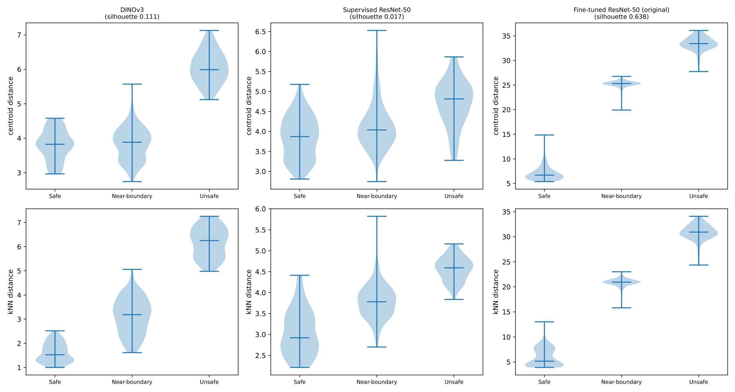
DINOv3 assigns nearly identical mean centroid distances to safe and near-boundary states (3.805 and 3.842) and a markedly larger distance to unsafe states (6.056): globally, near-boundary states sit inside the safe distribution and only lava-occupying states stand apart. The kNN distances tell a different story at the local scale, separating safe from near-boundary states by roughly a factor of two (1.613 versus 3.123). This local-global discrepancy is the central geometric observation of the study, and it is not an artifact of duplication.

The frozen ResNet-50 instead produces a monotonic gradient in both measures (centroid 3.852 → 4.124 → 4.713; kNN 3.044 → 3.787 → 4.566), but the increments are small: its safe and near-boundary classes are barely distinguished at either scale. The fine-tuned ResNet-50 separates the classes by an order of magnitude more (centroid 6.975 → 25.237 → 33.374), as expected for a model optimized on these labels; absolute magnitudes are not comparable across models of different dimensionality, so only the within-model pattern is interpretable.

Figure 4 shows the full distance distributions behind these means, and silhouette scores over the three classes on the same deduplicated embeddings quantify how well-separated the classes are globally: 0.111 for DINOv3, 0.017 for the frozen ResNet-50, and 0.638 for the fine-tuned model. Both frozen encoders therefore have heavily overlapping classes in the global geometry, with DINOv3 roughly six times better separated than the frozen ResNet-50 but still far from clean clusters. Whatever structure the probes exploit in the frozen encoders is local, not a global partition of the feature space.

Model	Safety state	Mean centroid distance	Mean kNN distance (k = 5)
DINOv3 (frozen)	Safe	3.805	1.613
DINOv3 (frozen)	Near-boundary	3.842	3.123
DINOv3 (frozen)	Unsafe	6.056	6.170
ResNet-50 (frozen)	Safe	3.852	3.044
ResNet-50 (frozen)	Near-boundary	4.124	3.787
ResNet-50 (frozen)	Unsafe	4.713	4.566
ResNet-50 (fine-tuned)	Safe	6.975	5.909
ResNet-50 (fine-tuned)	Near-boundary	25.237	20.863
ResNet-50 (fine-tuned)	Unsafe	33.374	30.826

Classification on held-out layouts and episodes

Table 3 reports the main evaluation: probes fitted on the 598 unique outer-training states and evaluated once on each held-out test set. The results separate sharply by comparison, and this separation is the study’s principal finding.

On the two comparisons that involve the unsafe class, all three feature extractors are essentially perfect on both test sets (accuracy ≥ 0.913, AUROC ≥ 0.996, and mostly exactly 1.0). On the safe-versus-near-boundary comparison, which requires distinguishing two classes that differ only in the agent’s distance to a boundary and not in any distinctive texture, the encoders diverge dramatically. On held-out layouts, DINOv3 classifies all 655 states correctly (balanced accuracy 1.000), and the fine-tuned ResNet-50 makes 2 errors (balanced accuracy 0.944). The frozen ImageNet ResNet-50 reaches 0.974 accuracy, which is barely above the 0.9725 majority-class baseline, and its balanced accuracy of 0.528 reveals why: it correctly identifies only 1 of the 18 held-out-layout safe states, classifying almost every state as near-boundary. The same ordering holds on the deduplicated held-out-episode set (DINOv3 1 error in 95, balanced accuracy 0.993; frozen ResNet-50 10 errors, balanced accuracy 0.737).

Repeating the episode-level holdout over five seeds confirms the stability of this gap. For safe versus near-boundary, DINOv3 attains a mean balanced accuracy of 0.996 ± 0.006 and the fine-tuned model 1.000 ± 0.000, while the frozen ResNet-50 attains 0.770 ± 0.157; for near-boundary versus unsafe the corresponding figures are 1.000 ± 0.000, 1.000 ± 0.000, and 0.732 ± 0.141. The frozen ResNet-50’s variance is an order of magnitude larger than either alternative on every comparison. These sets are small and their composition varies across seeds (8 to 179 states per comparison, with one seed lacking enough safe states for two comparisons), so the standard deviations describe stability rather than narrow confidence intervals.

Model	Test set	Safe vs. near-boundary	Safe vs. unsafe	Near-boundary vs. unsafe
DINOv3 (frozen)	Held-out layouts	1.0000 / 1.000 / 0	1.0000 / 1.000 / 0	1.0000 / 1.000 / 0
DINOv3 (frozen)	Held-out episodes	0.9895 / 0.993 / 1	1.0000 / 1.000 / 0	1.0000 / 1.000 / 0
ResNet-50 (fine-tuned)	Held-out layouts	0.9969 / 0.944 / 2	1.0000 / 1.000 / 0	1.0000 / 1.000 / 0
ResNet-50 (fine-tuned)	Held-out episodes	1.0000 / 1.000 / 0	1.0000 / 1.000 / 0	1.0000 / 1.000 / 0
ResNet-50 (frozen)	Held-out layouts	0.9740 / 0.528 / 17	0.9556 / 0.944 / 2	0.9970 / 0.963 / 2
ResNet-50 (frozen)	Held-out episodes	0.8947 / 0.737 / 10	0.9130 / 0.947 / 2	0.9750 / 0.750 / 2
Majority baseline	Held-out layouts	0.9725 / 0.500 / 18	0.6000 / 0.500 / 18	0.9593 / 0.500 / 27
Majority baseline	Held-out episodes	0.8000 / 0.500 / 19	0.8261 / 0.500 / 4	0.9500 / 0.500 / 4

Control conditions

Table 4 applies the identical pipeline to raw downsampled pixels and to a randomly initialized ResNet-50. The controls settle which of the comparisons are informative.

The randomly initialized ResNet-50 detects the unsafe class almost as well as the pre-trained encoders: on held-out layouts it reaches balanced accuracy 0.981 for safe versus unsafe and 0.959 for near-boundary versus unsafe, having never been trained on anything. Raw 32×32 grayscale pixels match it on near-boundary versus unsafe (balanced accuracy 0.957, AUROC 0.979) but not on safe versus unsafe (0.676), which is unsurprising given that grayscale downsampling discards lava’s distinctive hue and that this comparison has only 45 test states. Taken together, detecting lava requires no learned representation at all: an untrained network suffices. The near-perfect unsafe-class numbers reported for every encoder in this study, and in the original submission, therefore carry no evidence about representation quality, which confirms the visual-confound hypothesis for the unsafe class specifically.

The safe-versus-near-boundary comparison behaves in the opposite way. Neither control recovers the minority class on held-out layouts: raw pixels identify 0 of 18 safe states (balanced accuracy 0.493) and random features 8 of 18 (0.699), against 18 of 18 for DINOv3. On held-out episodes the AUROC gap is equally clear (0.711 for raw pixels and 0.760 for random features, versus 0.997 for DINOv3). This comparison is therefore not solvable from surface appearance or from architecture alone, and the performance DINOv3 achieves on it is attributable to what pre-training learned.

Features	Test set	Safe vs. near-boundary	Safe vs. unsafe	Near-boundary vs. unsafe
Raw pixels (32×32 gray)	Held-out layouts	0.9588 / 0.493 / 27	0.7333 / 0.676 / 12	0.9849 / 0.957 / 10
Raw pixels (32×32 gray)	Held-out episodes	0.7263 / 0.711 / 26	0.7391 / 0.645 / 6	0.8500 / 0.684 / 12
Random-weight ResNet-50	Held-out layouts	0.9405 / 0.699 / 39	0.9778 / 0.981 / 1	0.9895 / 0.959 / 7
Random-weight ResNet-50	Held-out episodes	0.6211 / 0.605 / 36	0.9130 / 0.750 / 2	0.9875 / 0.875 / 1
DINOv3 (for reference)	Held-out layouts	1.0000 / 1.000 / 0	1.0000 / 1.000 / 0	1.0000 / 1.000 / 0
DINOv3 (for reference)	Held-out episodes	0.9895 / 0.993 / 1	1.0000 / 1.000 / 0	1.0000 / 1.000 / 0

Anomaly detection

Applying the One-Class SVM protocol to all three encoders, with the detector fitted only on deduplicated outer-training safe states and evaluated on held-out states, reproduces the same ordering (Table 5). DINOv3 attains AUROC 0.975 for safe versus near-boundary and 1.000 for safe versus unsafe; the fine-tuned ResNet-50 attains 0.9998 and 1.000. The frozen ResNet-50 falls far behind at 0.750 and 0.889, close to chance on the near-boundary comparison. Because the detector never sees a non-safe label, this is the cleanest comparison in the study, and it places frozen self-supervised features much closer to a label-supervised model than to frozen ImageNet-supervised features. For reference, the contaminated fine-tuned model from the original submission scores a perfect 1.000 on both, illustrating the inflation that leakage produces.

Model	Safe vs. near-boundary (AUROC)	Safe vs. unsafe (AUROC)
DINOv3 (frozen)	0.9752	1.0000
ResNet-50 (fine-tuned, uncontaminated)	0.9998	1.0000
ResNet-50 (frozen)	0.7499	0.8894
ResNet-50 (fine-tuned, contaminated: original protocol)	1.0000	1.0000

Comparison with the original protocol

For transparency we record what the protocol used in the original submission produced: with a stratified random 70/30 timestep-level split, and with the external set of additional same-environment rollouts, every feature extractor reached accuracy and AUROC at or above 0.9920 on every comparison (DINOv3 and the fine-tuned model reached exactly 1.0000 in most cells, and the frozen ResNet-50 never fell below 0.9920 accuracy or 0.9995 AUROC). Under that protocol the three extractors appeared indistinguishable. Since 95.9% of that internal test set and 92.1% of the external set duplicate training states, the apparent equivalence was an artifact, and the frozen ResNet-50’s failure on the safe-versus-near-boundary comparison, a balanced accuracy of 0.528 on withheld layouts, was completely hidden. No conclusion in this paper rests on those numbers.

Balanced-sampling check

Subsampling outer-train to 80 safe, 80 near-boundary, and 40 unsafe unique states leaves the lava comparisons unchanged (DINOv3 stays at 1.000 accuracy on both). On safe versus near-boundary, DINOv3’s balanced accuracy falls from 1.000 to 0.850 on held-out layouts while the frozen ResNet-50 remains near chance (0.552). Because balancing discards roughly 85% of the training data, this is better read as a small-sample effect than as evidence that imbalance distorted the main results; the ordering between encoders is unchanged.

UMAP visualization

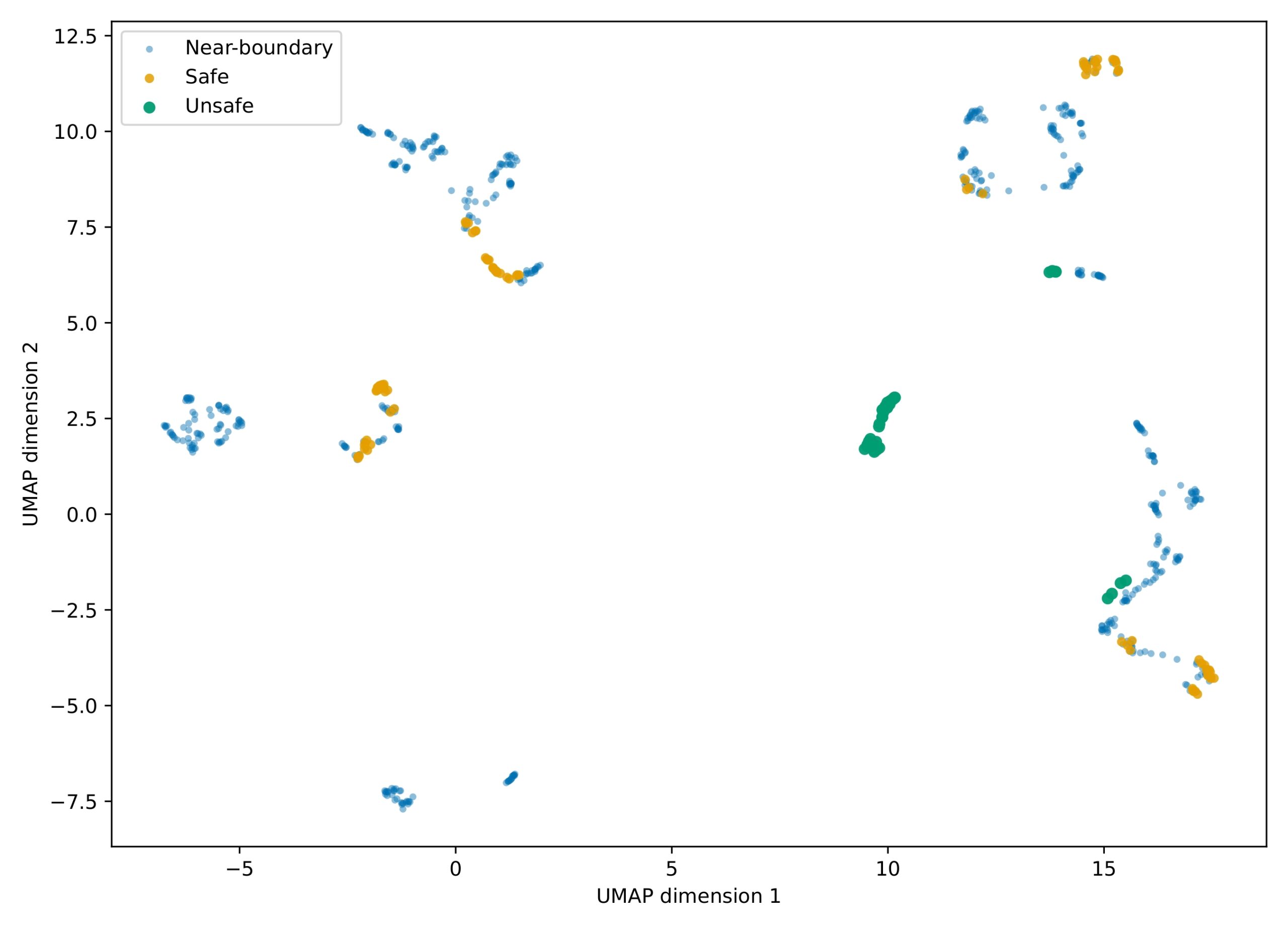
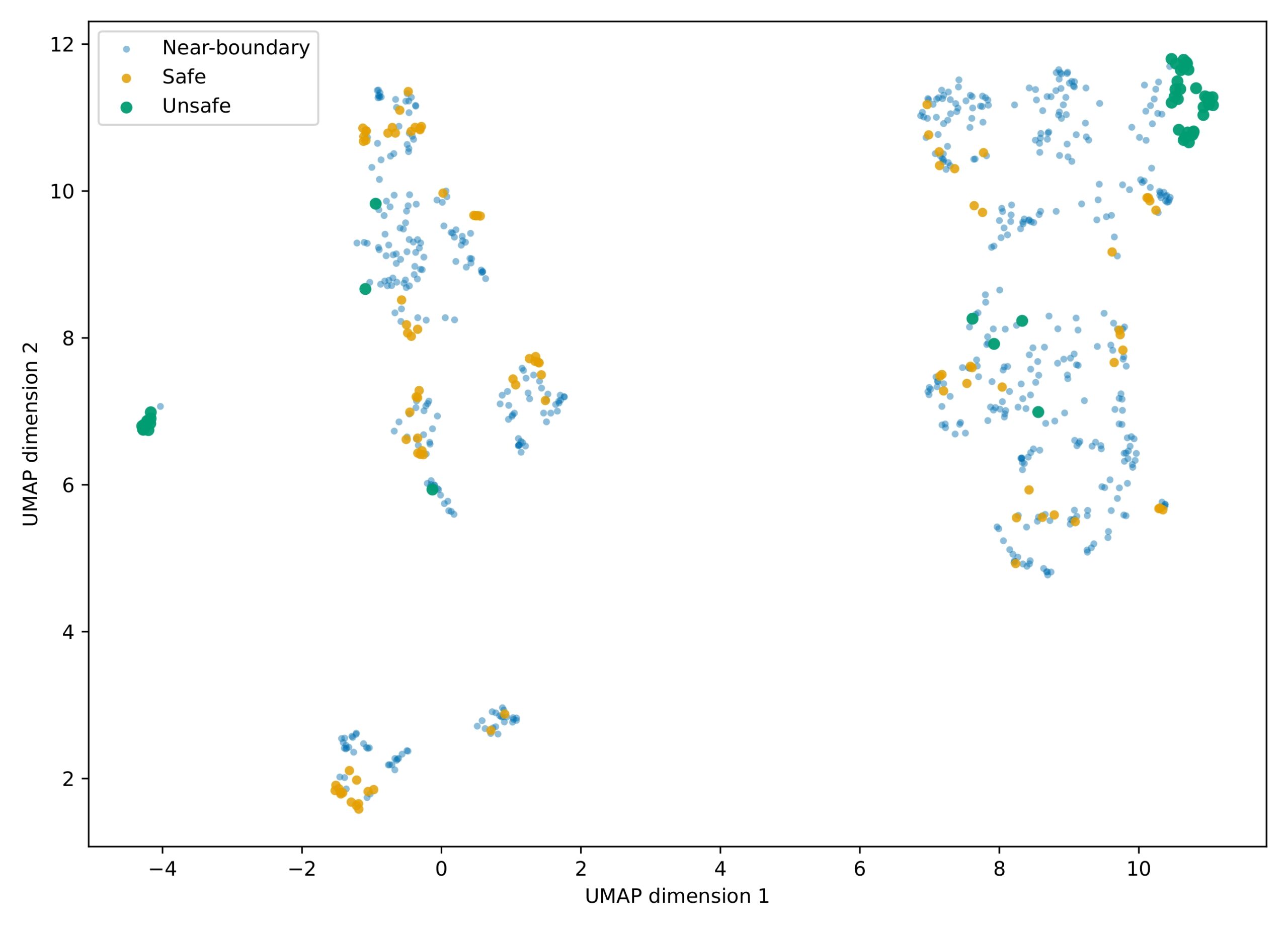
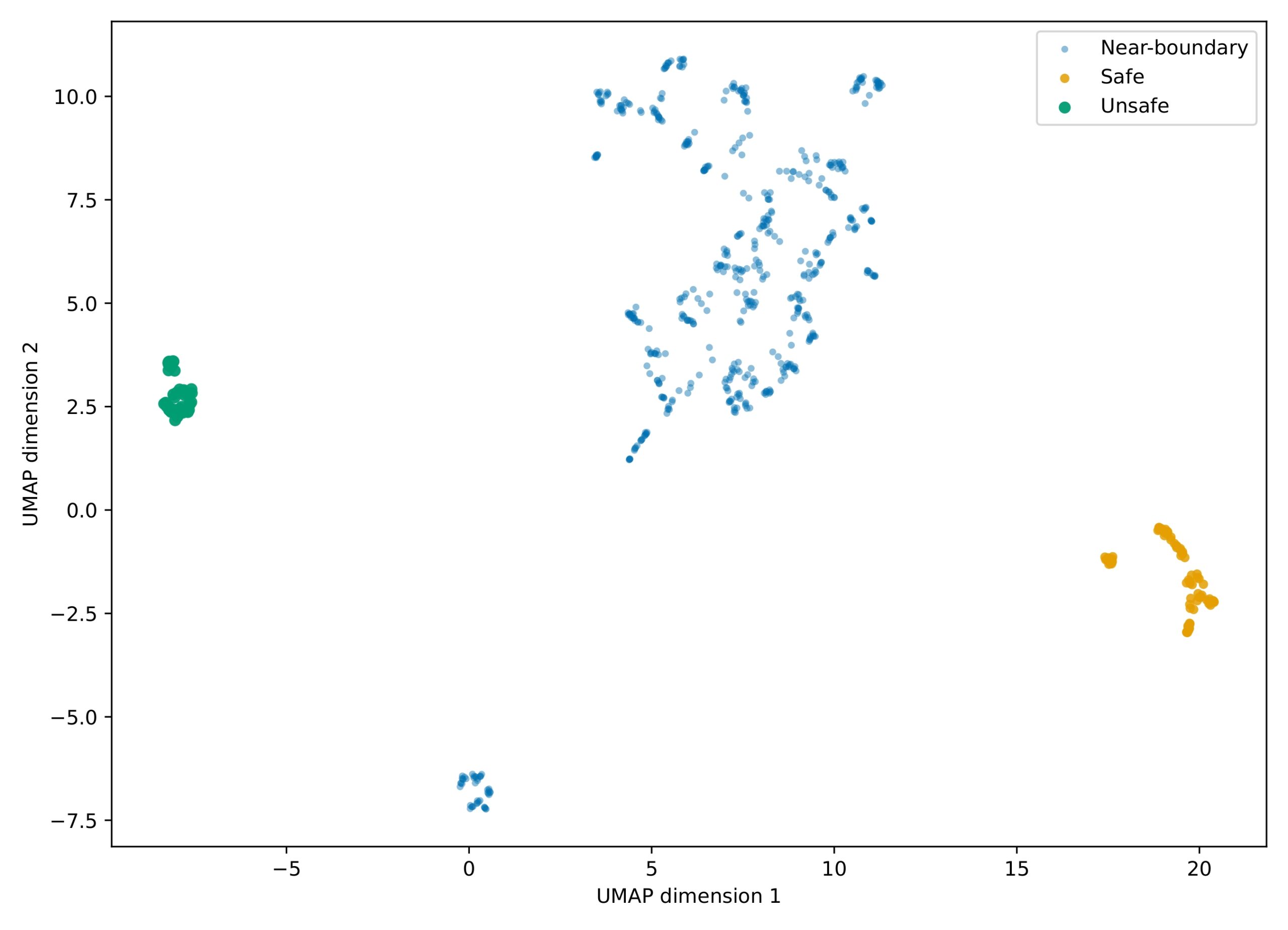
Figures 1-3 show two-dimensional UMAP projections of the three deduplicated feature spaces, and they track the silhouette scores closely. The fine-tuned ResNet-50 (Figure 3, silhouette 0.638) resolves into three cleanly separated regions, one per class, as expected for a model optimized on these labels. Neither frozen encoder does. In the DINOv3 projection (Figure 1, silhouette 0.111) the unsafe states form two compact clusters and the safe states form several small, tight clumps distributed across the projection rather than one region, each embedded among near-boundary points: locally grouped, globally interleaved. This is the two-dimensional signature of the local-global discrepancy measured in Table 2, and it is precisely why the probe results matter, since a boundary that separates these classes exists in the feature space but is not visible as a global partition. In the frozen ResNet-50 projection (Figure 2, silhouette 0.017) the unsafe states largely cluster but several fall inside near-boundary regions, and the safe states are thoroughly mixed throughout, with no local grouping comparable to DINOv3’s. We treat these projections as qualitative illustrations: UMAP preserves local neighborhoods at the expense of global distances, so the absence of visible separation is not by itself evidence of absent structure.

Discussion

Restatement of key findings

Three findings emerge once duplication and contamination are removed. First, the unsafe class is a visual artifact: a randomly initialized network, trained on nothing, detects lava nearly as well as any pre-trained encoder, and raw grayscale pixels match it on one of the two lava comparisons, so the near-perfect unsafe-class numbers that dominated our original submission, and that motivated its central claim, carry no information about representation quality. Second, the safe-versus-near-boundary distinction is genuinely difficult, and on it the two frozen encoders diverge sharply: on layouts never seen in training, frozen DINOv3 identifies all 18 held-out safe states while the frozen ImageNet ResNet-50 identifies 1, performing no better than always predicting the majority class despite an accuracy of 0.974. Frozen DINOv3 matches a ResNet-50 fine-tuned on the labels themselves (18 of 18 versus 16 of 18) without ever seeing a safety label. Third, the two frozen encoders organize the classes differently: DINOv3 places safe and near-boundary states at nearly identical distances from the safe centroid while separating them locally, whereas the frozen ResNet-50 produces a shallow monotonic gradient in which neither scale distinguishes them well.

The supportable claim is therefore narrower than the one we originally made, and better supported. We cannot conclude that frozen encoders represent safety: our labels are deterministic functions of visible geometry, and the hazard class is solvable from raw pixels. What the corrected evaluation establishes is that frozen self-supervised features expose a spatial relation, agent-to-boundary proximity, that is recoverable neither from surface appearance, nor from a random network of the same architecture, nor from ImageNet-supervised features of comparable capacity, and that this transfers to unseen layouts.

Why the two frozen encoders diverge

The divergence is consistent across three independent measurements: the probes (balanced accuracy 1.000 versus 0.528 on held-out layouts), the label-free anomaly detector (AUROC 0.975 versus 0.750), and the geometry (silhouette 0.111 versus 0.017). Since it appears in an experiment using no safety labels, it cannot be attributed to probe overfitting.

We cannot attribute it to self-supervision as such. DINOv3 and ResNet-50 differ simultaneously in architecture (ViT versus CNN), pre-training corpus (LVD-1689M versus ImageNet-1K), and objective (self-distillation versus label supervision), and our design cannot separate these. The random-weight control does exclude one candidate explanation: a randomly initialized ResNet-50 recovers 8 of 18 held-out safe states, more than the ImageNet-pretrained one, so the frozen ResNet-50’s failure is not an architectural limitation but something its supervised pre-training does to the features. A plausible reading, which our design can suggest but not test, is that ImageNet classification training discards the spatial layout information that survives in self-distilled patch-level features, and that the discarded information is exactly what a proximity label requires. Matched comparisons, a supervised ViT-B and a self-supervised ResNet-50, would test this directly and are the natural next experiment.

The visual confound, resolved for one class and not the other

Our original submission raised the visual distinctiveness of lava as a limitation and deferred the test. The controls now settle it, and more usefully than a single verdict: the confound is decisive for the unsafe class and absent for the safe-versus-near-boundary distinction. Lava is a visually distinctive tile appearing nowhere else in the environment, so even an untrained convolutional network separates it (balanced accuracy 0.981 for safe versus unsafe on held-out layouts), and 32×32 grayscale pixels suffice on near-boundary versus unsafe (0.979 AUROC) despite discarding its hue. Near-boundary states carry no such cue, being distinguished from safe states only by the agent’s distance to a wall or lava cell, and there both controls fail while DINOv3 does not.

This does not make the surviving result a demonstration of safety understanding. The distinction that survives the controls is still a static, position-derived one; a probe that solves it has learned to read spatial configuration, not consequences. Testing the stronger claim requires dissociating appearance from risk in both directions, for instance by recoloring lava to match the floor so that danger is inferable only from position, by adding hazardous ordinary-looking tiles, or by conditioning labels on orientation and planned action. We provide a script for the recolored-lava condition with the released code; running it is the immediate next step rather than a distant one.

Implications and significance

The practical implication is a caution about evaluation. Under our original protocol all three feature extractors scored above 0.99 everywhere and appeared interchangeable; once layouts are withheld and duplicates removed, one collapses on the only comparison not solvable from appearance. In small deterministic environments, train/test duplication is the default outcome of random splitting rather than an incidental flaw, and accuracy on an imbalanced test set can hide complete failure on the minority class. Balanced accuracy, majority baselines, and trivial-feature controls turned an uninformative result into a specific one.

As speculation, and no more than that, given that these observations come from a 7×7 gridworld: the geometric contrast may matter for how a representation is used downstream. DINOv3’s organization, in which near-boundary states are separated from the safe set locally without being globally distant from it, is the kind of structure nearest-neighbor and one-class detectors exploit, as used for runtime failure detection, and its advantage over the frozen ResNet-50 does persist in exactly that experiment (AUROC 0.975 versus 0.750)¹⁴. A smooth global gradient of the sort the frozen ResNet-50 exhibits is what barrier-function methods assume^36,37, but our results indicate its gradient is too shallow to be useful here. Any such guidance would need validation far beyond this environment.

Connection to objectives

Returning to our research questions: of the two frozen encoders, only DINOv3 supports a lightweight probe on the comparison the controls show to be non-trivial, and it does so on withheld layouts (Q1). The two encoders differ substantially rather than performing equivalently as our original leaky split suggested, favoring the self-supervised encoder, which matches a label-supervised model, though the three-way confound prevents attributing this to self-supervision specifically (Q2). The geometry is binary for DINOv3, with a local-global discrepancy that survives deduplication, and a shallow gradient for the frozen ResNet-50; both show weak global class separation (Q3).

Limitations

First, the held-out test sets are small: 18 safe states on held-out layouts and 99 unique states across all classes on held-out episodes. This is a hard ceiling imposed by an environment that admits only 732 distinct states, and it means individual percentages carry wide uncertainty; the frozen ResNet-50’s failure (1 of 18) and DINOv3’s success (18 of 18) are far apart, but finer distinctions between DINOv3 and the fine-tuned model are not resolvable at this sample size.

Second, the safety label remains a static, position-based proxy that merges wall and lava proximity, is dominated by wall adjacency (3,127 of 4,469 near-boundary states), and ignores orientation, action, and time horizon. It measures pixel-visible proximity, not trajectory-level safety. Third, the encoder comparison is confounded three ways, so no conclusion about self-supervision as a paradigm follows from it. Fourth, the environment is a single 7×7 gridworld explored by a random policy that crossed the gap in only 12.1% of episodes, leaving goal-side states sparsely covered. Fifth, results come from one environment family and one pair of checkpoints; whether the divergence we observe generalizes to other encoders or richer environments is untested. Finally, UMAP projections distort global distances and are used only illustratively.

Recommendations for future research

The most informative next experiment is the recolored-lava condition, which removes the texture cue while preserving the labels and would test whether the surviving result depends on any appearance cue at all. Second, matched comparisons (a supervised ViT-B and a self-supervised ResNet-50) would deconfound architecture, data, and objective. Third, larger grids or varied obstacle geometries would relieve the state-space ceiling that limits statistical resolution here. Fourth, replacing the static proxy with an action-conditioned outcome, such as the probability of failure within a horizon under a stated policy, would move the target from proximity toward safety proper. Finally, connecting representational geometry to downstream safety filtering would test whether the contrast we measure has practical consequences^36,37.

Closing thought

Our first analysis concluded that all three feature extractors were equivalent and that safety-relevant structure was everywhere. Both conclusions dissolved under a stricter protocol, and what replaced them is narrower but more informative: in a small gridworld, frozen self-supervised features expose a spatial relation that supervised ImageNet features do not, on the one comparison trivial features cannot solve. The distance between those conclusions is a reminder that in small deterministic environments the protocol can determine the finding as much as the representation does, and that controls establishing what a task does not require are often what make the remaining result worth reporting.

References

1. Y. Liu, W. Chen, Y. Bai, X. Liang, G. Li, W. Gao, L. Lin. Aligning cyber space with physical world: a comprehensive survey on embodied AI. arXiv preprint arXiv:2407.06886, 2024, https://arxiv.org/abs/2407.06886. [↩] [↩]
2. J. Duan, S. Yu, H. L. Tan, H. Zhu, C. Tan. A survey of embodied AI: from simulators to research tasks. IEEE Transactions on Emerging Topics in Computational Intelligence. Vol. 6 (2), pg. 230-244, 2022, https://arxiv.org/abs/2103.04918. [↩] [↩]
3. H. Saeidi, J. D. Opfermann, M. Kam, S. Wei, S. Leonard, M. H. Hsieh, J. U. Kang, A. Krieger. Autonomous robotic laparoscopic surgery for intestinal anastomosis. Science Robotics. Vol. 7 (62), eabj2908, 2022, https://doi.org/10.1126/scirobotics.abj2908. [↩] [↩]
4. R. Gassert, V. Dietz. Rehabilitation robots for the treatment of sensorimotor deficits: a neurophysiological perspective. Journal of NeuroEngineering and Rehabilitation. Vol. 15, 46, 2018, https://doi.org/10.1186/s12984-018-0383-x. [↩] [↩]
5. L. Chen, P. Wu, K. Chitta, B. Jaeger, A. Geiger, H. Li. End-to-end autonomous driving: challenges and frontiers. IEEE Transactions on Pattern Analysis and Machine Intelligence. Vol. 46 (12), pg. 10164-10183, 2024, https://doi.org/10.1109/TPAMI.2024.3435937. [↩]
6. Q. Bouniot. Towards few-annotation learning in computer vision: application to image classification and object detection tasks. Doctoral thesis, Université Jean Monnet Saint-Étienne, 2023, https://arxiv.org/abs/2311.04888. [↩]
7. R. Jiao, et al. Label-efficient deep learning in medical image analysis: challenges and future directions. arXiv preprint arXiv:2303.12484, 2023, https://arxiv.org/abs/2303.12484. [↩]
8. Q. Huang, T. Zhao. Data collection and labeling techniques for machine learning. arXiv preprint arXiv:2407.12793, 2024, https://arxiv.org/abs/2407.12793. [↩]
9. C. M. Lee, et al. Minority reports: balancing cost and quality in ground truth data annotation. arXiv preprint arXiv:2504.09341, 2025, https://arxiv.org/abs/2504.09341. [↩]
10. K. He, X. Chen, S. Xie, Y. Li, P. Dollar, R. Girshick. Masked autoencoders are scalable vision learners. arXiv preprint arXiv:2111.06377, 2021, https://arxiv.org/abs/2111.06377. [↩] [↩]
11. K. Nakamura, L. Peters, A. Bajcsy. Generalizing safety beyond collision-avoidance via latent-space reachability analysis. Robotics: Science and Systems (RSS), 2025, https://arxiv.org/abs/2502.00935. [↩] [↩]
12. Z. Wang, J. Hu, R. Mu. Safety of embodied navigation: a survey. Proceedings of the 34th International Joint Conference on Artificial Intelligence (IJCAI), 2025, https://doi.org/10.24963/ijcai.2025/1189. [↩] [↩] [↩] [↩]
13. J. Seo, K. Nakamura, A. Bajcsy. Uncertainty-aware latent safety filters for avoiding out-of-distribution failures (UNISafe). arXiv preprint arXiv:2505.00779, 2025, https://arxiv.org/abs/2505.00779. [↩] [↩]
14. C. Xu, T. K. Nguyen, E. Dixon, C. Rodriguez, P. Miller, R. Lee, P. Shah, R. Ambrus, H. Nishimura, M. Itkina. Can we detect failures without failure data? Uncertainty-aware runtime failure detection for imitation learning policies (FAIL-Detect). Robotics: Science and Systems (RSS), 2025, https://arxiv.org/abs/2503.08558. [↩] [↩] [↩]
15. O. Siméoni, H. V. Vo, M. Seitzer, et al. DINOv3. arXiv preprint arXiv:2508.10104, 2025, https://arxiv.org/abs/2508.10104. [↩] [↩] [↩]
16. K. He, X. Zhang, S. Ren, J. Sun. Deep residual learning for image recognition (ResNet). IEEE Conference on Computer Vision and Pattern Recognition (CVPR), pg. 770-778, 2016, https://arxiv.org/abs/1512.03385. [↩] [↩]
17. R. Balestriero, et al. A cookbook of self-supervised learning. arXiv preprint arXiv:2304.12210, 2023, https://arxiv.org/abs/2304.12210. [↩] [↩] [↩] [↩] [↩] [↩] [↩] [↩] [↩] [↩]
18. T. Chen, S. Kornblith, M. Norouzi, G. Hinton. A simple framework for contrastive learning of visual representations (SimCLR). Proceedings of the 37th International Conference on Machine Learning (ICML), PMLR. Vol. 119, pg. 1597-1607, 2020, https://arxiv.org/abs/2002.05709. [↩]
19. S. A. Koohpayegani, A. Tejankar, H. Pirsiavash. Mean Shift for self-supervised learning (MSF). IEEE/CVF International Conference on Computer Vision (ICCV), 2021, https://arxiv.org/abs/2105.07269. [↩]
20. D. Dwibedi, Y. Aytar, J. Tompson, P. Sermanet, A. Zisserman. With a little help from my friends: nearest-neighbor contrastive learning of visual representations (NNCLR). IEEE/CVF International Conference on Computer Vision (ICCV), 2021, https://arxiv.org/abs/2104.14548. [↩]
21. J. Y. Lim, K. M. Lim, C. P. Lee, Y. X. Tan. SCL: self-supervised contrastive learning for few-shot image classification. Neural Networks. Vol. 165, pg. 19-30, 2023, https://doi.org/10.1016/j.neunet.2023.05.037. [↩]
22. J.-B. Grill, et al. Bootstrap your own latent: a new approach to self-supervised learning (BYOL). Advances in Neural Information Processing Systems (NeurIPS), 2020, https://arxiv.org/abs/2006.07733. [↩]
23. M. Caron, H. Touvron, I. Misra, H. Jegou, J. Mairal, P. Bojanowski, A. Joulin. Emerging properties in self-supervised vision transformers (DINO). IEEE/CVF International Conference on Computer Vision (ICCV), 2021, https://arxiv.org/abs/2104.14294. [↩]
24. D. Hafner, T. Lillicrap, I. Fischer, R. Villegas, D. Ha, H. Lee, J. Davidson. Learning latent dynamics for planning from pixels (PlaNet). Proceedings of the 36th International Conference on Machine Learning (ICML), PMLR. Vol. 97, pg. 2555-2565, 2019, https://arxiv.org/abs/1811.04551. [↩]
25. A. Bardes, Q. Garrido, J. Ponce, X. Chen, M. Rabbat, Y. LeCun, M. Assran, N. Ballas. Revisiting feature prediction for learning visual representations from video (V-JEPA). Transactions on Machine Learning Research (TMLR), 2024, https://arxiv.org/abs/2404.08471. [↩]
26. G. Zhou, H. Pan, Y. LeCun, L. Pinto. DINO-WM: world models on pre-trained visual features enable zero-shot planning. arXiv preprint arXiv:2411.04983, 2024, https://arxiv.org/abs/2411.04983. [↩] [↩]
27. A. Dosovitskiy, et al. An image is worth 16×16 words: transformers for image recognition at scale (ViT). International Conference on Learning Representations (ICLR), 2021, https://arxiv.org/abs/2010.11929. [↩]
28. A. Radford, et al. Learning transferable visual models from natural language supervision (CLIP). International Conference on Machine Learning (ICML), 2021, https://arxiv.org/abs/2103.00020. [↩]
29. Y. Bengio, A. Courville, P. Vincent. Representation learning: a review and new perspectives. IEEE Transactions on Pattern Analysis and Machine Intelligence. Vol. 35 (8), pg. 1798-1828, 2013, https://arxiv.org/abs/1206.5538. [↩]
30. G. E. Hinton, R. R. Salakhutdinov. Reducing the dimensionality of data with neural networks. Science. Vol. 313 (5786), pg. 504-507, 2006, https://doi.org/10.1126/science.1127647. [↩]
31. D. Ha, J. Schmidhuber. Recurrent world models facilitate policy evolution. Advances in Neural Information Processing Systems (NeurIPS), 2018, https://arxiv.org/abs/1803.10122. [↩]
32. S. Nair, A. Rajeswaran, V. Kumar, C. Finn, A. Gupta. R3M: a universal visual representation for robot manipulation. Conference on Robot Learning (CoRL), 2022, https://arxiv.org/abs/2203.12601. [↩]
33. T. Xiao, I. Radosavovic, T. Darrell, J. Malik. Masked visual pre-training for motor control (MVP). arXiv preprint arXiv:2203.06173, 2022, https://arxiv.org/abs/2203.06173. [↩]
34. P. Sermanet, et al. Generating robot constitutions & benchmarks for semantic safety (ASIMOV benchmark). arXiv preprint arXiv:2503.08663, 2025, https://arxiv.org/abs/2503.08663. [↩]
35. C. Guo, G. Pleiss, Y. Sun, K. Q. Weinberger. On calibration of modern neural networks. Proceedings of the 34th International Conference on Machine Learning (ICML), PMLR. Vol. 70, pg. 1321-1330, 2017, https://arxiv.org/abs/1706.04599. [↩]
36. K. Nakamura, A. L. Bishop, S. Man, A. M. Johnson, Z. Manchester, A. Bajcsy. How to train your latent control barrier function: smooth safety filtering under hard-to-model constraints (LatentCBF). arXiv preprint arXiv:2511.18606, 2025, https://arxiv.org/abs/2511.18606. [↩] [↩] [↩]
37. Z. Sun, S. Song. Latent policy barrier: learning robust visuomotor policies by staying in-distribution (LPB). Advances in Neural Information Processing Systems (NeurIPS), 2025, https://arxiv.org/abs/2508.05941. [↩] [↩] [↩]
38. G. Alain, Y. Bengio. Understanding intermediate layers using linear classifier probes. arXiv preprint arXiv:1610.01644, 2016, https://arxiv.org/abs/1610.01644. [↩]
39. Y. Sun, Y. Ming, X. Zhu, Y. Li. Out-of-distribution detection with deep nearest neighbors. Proceedings of the 39th International Conference on Machine Learning (ICML), PMLR. Vol. 162, 2022, https://arxiv.org/abs/2204.06507. [↩]
40. M. Chevalier-Boisvert, B. Dai, M. Towers, R. de Lazcano, L. Willems, S. Lahlou, S. Pal, P. S. Castro, J. Terry. Minigrid & Miniworld: modular & customizable reinforcement learning environments for goal-oriented tasks. Advances in Neural Information Processing Systems (NeurIPS), Datasets and Benchmarks Track, 2023, https://arxiv.org/abs/2306.13831. [↩] [↩]
41. P.-N. Tan, M. Steinbach, A. Karpatne, V. Kumar. Introduction to data mining (2nd ed.). Pearson, 2018. [↩]
42. A. Paszke, et al. PyTorch: an imperative style, high-performance deep learning library. Advances in Neural Information Processing Systems (NeurIPS), 2019, https://arxiv.org/abs/1912.01703. [↩] [↩] [↩]
43. T. M. Cover, P. E. Hart. Nearest neighbor pattern classification. IEEE Transactions on Information Theory. Vol. 13 (1), pg. 21-27, 1967, https://doi.org/10.1109/TIT.1967.1053964. [↩]
44. B. Schölkopf, J. C. Platt, J. Shawe-Taylor, A. J. Smola, R. C. Williamson. Estimating the support of a high-dimensional distribution. Neural Computation. Vol. 13 (7), pg. 1443-1471, 2001, https://doi.org/10.1162/089976601750264965. [↩]
45. L. McInnes, J. Healy, J. Melville. UMAP: uniform manifold approximation and projection for dimension reduction. arXiv preprint arXiv:1802.03426, 2018, https://arxiv.org/abs/1802.03426. [↩] [↩]