A Dual-Model Autoregressive Forecasting Framework for Renewable Energy Demand, Generation, and Power Imbalance Analysis

Abstract

The intermittent nature of solar and wind generation creates a mismatch between supply and demand that has been a major impediment to the reliability and efficiency of our nation’s power grid. To compensate for these mismatches, grid operators have had to utilize additional sources of generation to ensure system stability. The purpose of this research is to investigate if an Autoregressive Model developed from actual hourly energy generation/demand data collected from the National Power Grid and weather/environmental data could accurately predict hourly energy generation/demand to aid in the analysis of the residual of the power grid. A total of 12 months of CAISO Net Load Data were used to develop an autoregressive model to forecast hourly energy demand, while renewable generation was forecasted by combining the CAISO Renewable Generation Data with the SolarAnywhere Environmental Irradiance Variables as Exogenous Inputs. All data sets were aligned, normalized and divided into two parts based on time (80% training data, 20% test data), and lagged features were created for forecasting. Both for energy generation and demand, we tested four different types of regression algorithms: MLPRegressor, SGDRegressor, Gaussian Process Regressor, and Random Forest Regressor. The best models were a two-layer Multilayer Perceptron (R²=0.84) for demand, and  Stochastic Gradient Descent Regressor with environmental inputs (R²=0.84) for generation. When integrated into an analysis of forecasted residuals (predicted demand minus generation), the system outperformed  the baseline single-window model by approximately 137% (R²=0.71). This combined model is used as a decisional framework, with positive and negative outputs suggesting to release or store energy in the grid, respectively. Unlike traditional models that rely on predicting net energy load directly, this study models supply and demand independently, introducing a more novel, efficient structure. The use of autoregressive models on top of complex deep learning frameworks gives us an approach with high interpretability, simplicity and good performance compared to previous methods.

Keywords: Renewable Energy Forecasting, Machine Learning, Smart Grids, Autoregressive Modeling, Energy Demand Forecasting, Renewable Generation Forecasting, Grid Residual Analysis

Introduction

In 2023, California curtailed over 2.4 million megawatt-hours (MWh) of renewable energy, largely due to midday solar oversupply¹. With an emphasis on using sustainable energy sources such as solar and wind, there is now a global movement to make renewable energy a significant part of how we produce our electricity. This transition to using sustainable energy has changed the design of today’s electrical networks by reshaping the topology, composition, and dynamics. Contemporary proliferation of renewable power generation is causing an overhaul in the topology, composition, and dynamics of electrical grids, with low-output, intermittent generators now widely distributed throughout the grid, including at the household level². Solar energy is the most prevalent energy source on Earth, and its economic efficiency and optimality is improving rapidly through increasing investments.  However, global decarbonization efforts require zero-carbon energy sources to be widely deployed by 2050 or 2060³, while fossil fuels still contributed 61.3% of global electricity generation in 2020⁴. Although renewable energy sources are essential for reducing greenhouse gas emissions, the forecastability of solar PV output is heavily influenced by weather conditions, such as rainy, cloudy, and sunny days⁵, introducing variability into grid operations. Solar irradiance changes with cloud cover and atmospheric conditions, while wind generation varies with changing weather patterns⁶. The intermittent nature and geographical limitations of solar and wind systems have increased interest in hybrid renewable energy solutions, yet the fundamental challenge of balancing electricity supply and demand remains⁷. Renewable energy sources are fundamentally intermittent, which means they rely on the availability of natural resources like the sun and wind rather than continuously producing energy. This creates frequent mismatches between electricity supply and demand that require grid operators to curtail excess generation or rely on energy storage systems⁸. Therefore, improving short-term forecasting accuracy is crucial for enhancing grid reliability and reducing energy waste.

Recent advances in machine learning (ML) and deep learning (DL) have allowed for the creation of forecasting systems capable of modeling the nonlinear temporal relationships that encapsulate renewable energy generation and demand. Forecasting has become an essential component of the power and energy industry, with researchers developing thousands of models for predicting electricity demand, prices, and renewable generation⁹. As renewable energy penetration continues to increase, accurate forecasting has become increasingly important for efficient grid operation and energy management, while the limitations of traditional forecasting methods have encouraged the adoption of ML and DL algorithms because of their ability to capture complex nonlinear patterns¹⁰. For solar power specifically, a comprehensive review of photovoltaic forecasting techniques has summarized methods ranging from physical models to neural network approaches¹¹, while ensemble learning methods combining extreme gradient boosting and deep neural networks have demonstrated effective forecasting of hourly solar irradiance¹². For wind forecasting, researchers have identified uncertainty as one of the primary barriers to large-scale grid integration and have shown that machine learning provides an effective forecasting approach ¹³. Wind power prediction based on high-frequency SCADA data combined with isolation forest preprocessing and deep learning neural networks has also demonstrated strong one-hour-ahead forecasting performance¹⁴. Comparisons of 24 machine learning models for day-ahead photovoltaic forecasting have further shown that model selection and hyperparameter tuning significantly affect prediction accuracy¹⁵. However, recent studies have also questioned whether increasingly complex architectures always improve forecasting performance, reporting that simpler linear models can outperform Transformer-based methods for long-term time-series forecasting¹⁶. Graph neural networks have demonstrated strong capability in modeling multivariate time-series data by exploiting latent spatial relationships ¹⁷, while the Informer architecture was introduced to efficiently capture long-range temporal dependencies in long-sequence forecasting problems¹⁸.

Energy demand forecasting presents equally important challenges for modern power systems. Global electricity demand for residential and commercial applications has continued to increase despite persistent inadequacies in electricity generation capacity¹⁹. Accurate electricity demand and price forecasting are essential for both market participants and system operators, yet forecasting remains difficult because of factors such as volatility, long-term trends, seasonal effects, calendar effects, and sudden demand spikes²⁰. Machine learning methods have become increasingly popular alternatives to traditional statistical techniques for short-term load forecasting ²¹. Smart grids have made accurate demand forecasting even more important, especially as artificial intelligence, big data, and the Internet of Things become more common in modern power systems²². As these technologies are adopted more widely, accurate forecasts help grid operators balance electricity supply and demand while keeping the grid stable and efficient²³. Deep learning models have shown strong potential for learning complex customer demand patterns across multiple forecasting horizons²⁴, while AI and ML have also emerged as important technologies for demand-side response because they enable near real-time decision-making using large-scale datasets²⁵.

Despite these advances, most existing approaches focus on forecasting net load directly or predicting renewable generation independently rather than separating electricity demand and renewable generation into distinct, interpretable models. Time-series modeling remains an effective approach for analyzing future power system performance using historical data²⁶, yet integrating independent demand and generation forecasts into operational decision-making remains relatively underexplored. The increasing penetration of renewable energy has made net-load forecasting an increasingly important challenge for power system planning and operation²⁷. In addition, accurate net-load forecasting is critical for quantifying uncertainty at the distribution level and supporting reliable grid operation²⁸. Renewable curtailment has also become a significant issue in many countries due to the rapid growth of wind and solar generation capacity²⁹. Researchers have explored forecasting, energy storage, and curtailment as ways to make better use of renewable energy³⁰. Large-scale battery storage can help balance electricity generation and demand, and lithium-ion batteries are commonly used because of their efficiency, long cycle life, and high energy density³¹. However, current forecasting frameworks rarely model supply-demand residuals as an explicit output that can directly support battery storage scheduling and grid management decisions.

This research examines if an auto-regressive Machine Learning model developed with actual grid and environmental data can forecast short term electricity demand, renewable generation, and provide operational power imbalance analysis. The method of forecasting electricity demand and renewable generation individually and then combining them for a power imbalance analysis is different than traditional methods which directly forecast net-load. Two forecasting problems were examined: (1) electricity demand forecasting using historical CAISO net-load data, and (2) renewable generation forecasting using CAISO renewable generation output and environmental predictors from SolarAnywhere. Random Forest, Gaussian Process Regression, SGD Regression, and Multi-Layer Perceptrons were used as machine learning models. These forecasts were then used to estimate when renewable energy production would be above or below demand, which provides support to guide battery storage, reduce unnecessary curtailment, and improve grid management.

Methodology

Overview of the Model

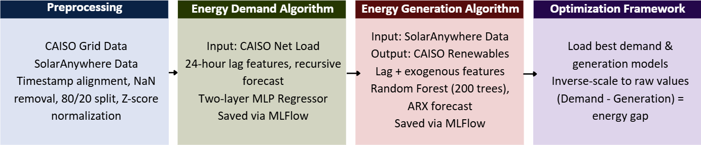
An overview of the process used for this algorithm is shown in Figure 1.

Data Acquisition

CAISO Hourly Standardized Dataset

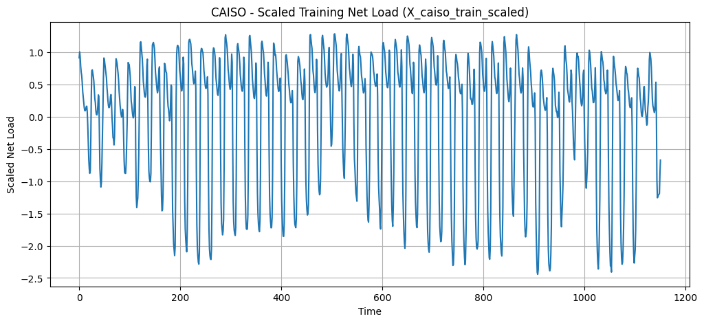
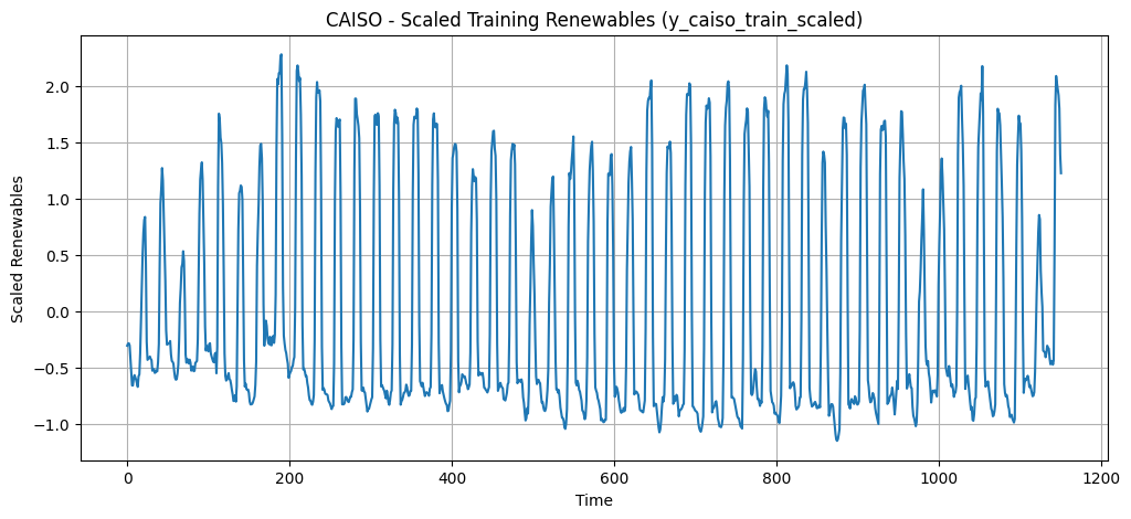
The California Independent System Operator (CAISO)³² standardized hourly dataset was used as the primary grid data source, as shown in Figure 2 and 3.

. The dataset provided:

• Total grid load, “net_load”, (MW) — used for demand forecasting
• Renewable generation values, “renewables”, (MW) — used for generation forecasting
• Hourly timestamps (PST)

One year worth of data (January 2025 – December 2025) was imported directly into Python using pandas and sorted chronologically to preserve time-series structure. Figure 2 presents the training data of CAISO Net load, and Figure 3 presents the training data of CAISO Renewables.

Solar Anywhere Dataset

To model renewable generation drivers, Solar Anywhere data were integrated³³. The following environmental variables were used:

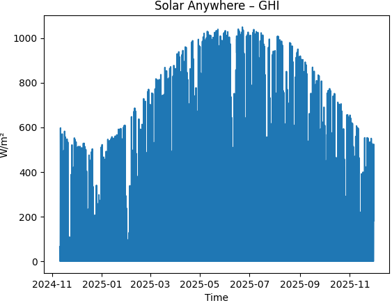
• Global Horizontal Irradiance, “GHI”, (W/m²), which measures the total solar radiation received on a horizontal surface. This data is graphed in Figure 4.
• Direct Normal Irradiance, “DNI”, (W/m²), which measures the amount of direct solar radiation received by a surface positioned perpendicular to the sun’s rays.
• Diffuse Horizontal Irradiance, “DHI”, (W/m²), which measures scattered solar radiation reaching the surface, especially under cloudy or shaded conditions.
• Air temperature, “temp_air”, (°C), which captures temperature changes that affect photovoltaic panel efficiency and electrical conversion performance.
• Wind speed, “wind_speed”, (m/s), which captures wind conditions that affect changes in renewable energy generation and photovoltaic panel temperature.

The selection of these variables is due to their direct impact on photovoltaic (PV) efficiency and therefore renewable energy production. The data used in this study was gathered from January 2025 – December 2025. Time stamp alignment with CAISO’s hourly interval allowed for the merging of data sets to provide a consistent time frame of analysis. Figure 4 represents the scaled training data for the Solar Anywhere GHI.

Data Preprocessing

The first step was to check for nulls/missing data and then clean them out of each of the datasets. After checking that all of the timestamp entries followed an hourly pattern (i.e., every hour there is a record), each of the datasets were sorted by time. Strict time ordering was maintained to prevent future data from influencing past predictions.

The data were then split 80/20 based on time, with the first 80 percent used for training and the final 20 percent used for testing. This approach replicates real-world forecasting while preventing data leakage from random sampling.

Feature scaling was performed using Z-score normalization:

where μ and σ are the mean and standard deviation calculated from the training data. The same values were then used to scale the test set.

Feature Engineering

Autoregressive Lag Construction

The CAISO Standardized Hourly Dataset for total grid load, or “net_load” (MW), was used to build the autoregressive demand model. For both forecasting tasks, lagged features were created using past values of the target variable. For a given time step,

where y_t-k represents the value of the target variable at lag k³⁴. The lag window size n was varied to test how it affected model performance. This allowed the models to account for patterns over time in electricity demand and renewable generation.

In addition to including environmental data at each timestep as an exogenous variable (variables that are in the same timeframe as the main time series), for renewable generation forecasting purposes, these variables were added to the formulation:

where X_t represents irradiance and weather-related features.

Recursive Multi-Step Forecasting

The SolarAnywhere environmental variables (GHI, DNI, DHI, air temperature, and wind speed) were used to predict renewable generation, or “renewables” (MW), from the CAISO Standardized Hourly Dataset. Recursive forecasting was used for multi-step predictions. The model first predicted one hour ahead and then used that prediction as a lag input for the following hour. This process was repeated across the forecast period, since the actual values for future time steps would not be available during real-world forecasting.

Model Development and Benchmarking

Four regression models were tested and compared. For the Random Forest Regressor, 200, 400, 800, and 1600 estimators were tested. Hyperparameters were chosen through manual experimental tuning, where a small set of reasonable values was tested and the configuration with the highest test R² was selected while also considering stable training behavior. In a Random Forest model, each estimator is an individual decision tree within the larger ensemble. Each tree is trained on a bootstrap sample of the data, and the predictions from all the trees are then averaged to produce the final output. The n_estimators parameter determines the number of decisional trees in the forest. In general, adding more trees helps reduce variance and makes the model’s predictions more stable. However, as the number of trees continues to increase, the improvements become smaller while the computational cost continues to grow.

The Gaussian Process Regression model was assessed as a way to represent non-linear relationships. However, it had a high computational burden and a lack of scalability. Conversely, the SGD Regressor was used as a computationally efficient linear base-line; the model’s parameters were optimized by iteratively performing stochastic gradient descent. The MLP model was evaluated based on architectures with one, two, or three hidden layers, and each hidden layer contained 100 neurons. Hyper-parameters such as the learning rate and number of iterations were determined experimentally to maximize model performance.

The models’ performance was measured by their Coefficient of Determination (R2), Mean Absolute Error (MAE) and Root Mean Square Error (RMSE). These three metrics provide an assessment of model performance from a quantitative perspective. Also, all three metrics meet the requirements of the established Engineering Research Plan. The final models that were used on the test data included a two layer multi-layer perceptron (MLP) autoregressive model to forecast energy demand; and a Stochastic Gradient Descent Regressor (SGDR) model with lagged input variables and environmental inputs to forecast renewable generation.

Analysis of Forecasted Residuals

Following independent training and benchmarking, the best-performing models for each forecasting task were selected: the two-layer MLP for energy demand and the SGDRegressor with lagged and environmental inputs for renewable generation. Then, both models were saved and combined to analyze the forecasted residuals. This framework evaluates real-world grid balancing performance by calculating the predicted power imbalance at each time step as the difference between predicted electricity demand and predicted renewable generation. The resulting imbalance indicates whether the grid is expected to experience a renewable energy surplus.

To align the timestamps, the predicted outputs from both models were flattened and synchronized using identical hourly timestamps. The predicted power imbalance was then compared against the actual observed imbalance using the coefficient of determination (R²), mean absolute error (MAE), and root mean square error (RMSE). This comparison made it possible to evaluate how forecasting errors propagate when the independently predicted supply and demand values are integrated.

Results

Energy Demand Model Experiments

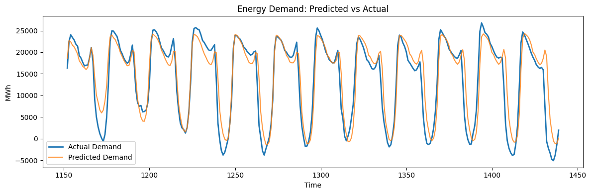
Table 1 compares the regression models tested for energy demand forecasting using a 24-hour autoregressive window and a time-based test set. For each experiment, the configuration with the highest test R² that also trained stably was selected. The Random Forest Regressor gave fairly consistent results as the number of trees increased from 200 to 1600. Its R² stayed around 0.55, and the MAE and RMSE changed only slightly between configurations. There was also little improvement after 200 trees, suggesting that adding more estimators was no longer providing much additional variance reduction. Gaussian Process Regression was also tested, but its performance was poor and resulted in negative R² values, so it was not included in the table. The SGD Regressor had high error values as well and did not generalize as well to the test data. The MLP models performed considerably better. The one-layer MLP reached an R² of 0.667, and increasing the network to two hidden layers improved the R² to 0.835, with an MAE of 2522.24 MW and an RMSE of 3786.94 MW. This was the strongest performance among the models tested. For context, California’s peak electricity demand is approximately 50,000 MW, so an average error of 2,522 MW is about 5% of peak demand. This provides the two-layer MLP with a comparatively small forecasting error when considering the total magnitude of electricity demand and makes it suitable for use as an operational forecasting tool for short-term applications. Adding a third hidden layer to the MLP degraded the performance of the model, which is likely a result of over-fitting. Based upon how well the two-layer MLP performed on the held-out test data, it was chosen as the energy demand forecasting model to be used in the analysis of residual forecasts. Figure 5 illustrates how closely the two-layer MLP followed the overall shape of the observed demand signal, capturing both daily demand cycle behaviors and extreme peak period events. Although a few deviations can be seen near the local maximums and minimums, the predicted values are generally aligned with the actual demand profile (i.e., demand over time), which demonstrates that the model has high time-based forecasting ability.

Model		R2	MAE (MW)	RMSE (MW)
SGDRegressor		0.23	6350	7530
MLP (1 Layer)		0.67	3615	4943
MLP (2 Layers)		0.84	2522	3786
MLP (3 Layers)		-13.3	26255	32374
Model	n_estimators
RandomForest	200	0.55	4065	5696
RandomForest	400	0.55	4077	5716
RandomForest	800	0.55	4135	5747
RandomForest	1600	0.55	4097	5721

Energy Generation Model Experiments

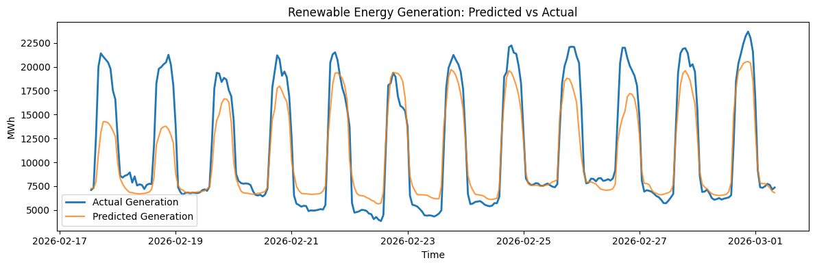
The renewable energy generation forecasting experiments were conducted on autoregressive models (ARX) where the independent variable is an environmental input. A 24-hour lag window was used for this model. As in the case of demand forecasting, the best performing model from the configuration that had stable training was chosen based upon its test R2 value. For the ensemble models, the Random Forest ARX with 200 estimators performed the best, achieving R² = 0.84, MAE = 1788.58 MW, and RMSE = 2542.39 MW, as shown in Table 2. However, increasing the number of estimators to 400 and 800 did not improve the results. R² slightly decreased, while both MAE and RMSE increased. This suggests that the Random Forest had already reached most of its performance improvement at 200 estimators, and adding more trees provided little additional benefit. Classical regression approaches showed mixed results: Gaussian Process Regression and MLP 2 layers performed poorly with negative R², and hence was not mentioned in the table; SGD Regressor achieved strong performance (R² = 0.76) as shown in Table 2. The three-layer configuration also underperformed relative to simpler architectures. These results indicate that, in terms of forecasting renewable generation with environmental inputs, the ensemble tree-based models exhibited the most advantageous combination of forecast accuracy and forecast stability. Based upon the held-out test data set performance of all the models evaluated in this study, the Random Forest ARX model using 200 estimators was identified as the preferred renewable generation forecasting model for use in the analysis of forecasted residuals. Figure 6 also provides an illustration of how well the Random Forest ARX model predicts renewable generation. The figure shows that the Random Forest ARX model is able to accurately predict the daily generation cycle of renewable energy sources as well as the major generation peaks. While the Random Forest ARX model may slightly underestimate certain peaks in renewable generation output during high renewable generation days, the predicted and observed renewable generation curves are generally aligned throughout the entire evaluation period which demonstrates a high degree of forecast stability under varying environmental conditions.

The renewable generation forecasts were produced using a recursive multi-step forecasting strategy, in which each predicted value was used as an input for subsequent forecast steps. Consequently, prediction errors may accumulate as the forecast horizon increases. The performance metrics reported in this study therefore represent the overall forecasting performance across the evaluation period rather than accuracy at individual forecast horizons.

Model		R2	MAE (MW)	RMSE (MW)
SGDRegressor		0.76	1788	2542
MLP (1 Layer)		0.73	2535	3.32E3
MLP (3 Layers)		0.51	3444	4.50E3
Model	n_estimators
RandomForest	200	0.84	2265	2902
RandomForest	400	0.78	2344	3003
RandomForest	800	0.78	2340	2999

Integrated Model Evaluation

The proposed autoregressive model was evaluated against a simple benchmark, which consisted of a Random Forest model trained on the previous hour’s renewable generation (a one-hour window) and no autoregressive lags or environmental predictors. As such, the simple recursive benchmark will allow for the separate evaluation of the contributions of longer time windows of historical data and the contribution of external weather-related factors. The simple benchmark produced an R2 of 0.31; thus, adding additional time windows of historical data as well as additional environmental variables significantly improves the overall forecasting accuracy. In a study on short-term load forecasting, LSTM-based models achieved R² values in the range of approximately 0.88–0.90 on normalized datasets³⁵. Feedforward ANN models reported R² values between 0.82 and 0.85³⁶. Interpretable Short Term Load Forecasting (STLF), or decomposition-based load forecasting model performed significantly weaker with a reported R² value of 0.52, as summarized in Table 3³⁷.

Model	R2	MAE (MW)	RMSE (MW)
This Study – Demand (MLP, 2-layer)	0.84	2522	3786
This Study – Generation (RF ARX 200)	0.84	1788	2542
This Study – Combined Power Imbalance (Jan-Apr)	0.71	3451	4569
This Study – Combined Power Imbalance (May-Aug)	0.71	3398	4555
This Study – Combined Power Imbalance (Sept-Dec)	0.70	3576	4609
Baseline – (RF 200 No ARX)	0.31	4955	6523
Interpretable STLF (Decomposition Model)	0.52	Normalized	Normalized
ANN (Feedforward NN)	0.82-89	Normalized	Normalized
LSTM	0.88-90	Normalized	Normalized

The two-layer autoregressive MLP demand model in this study achieved R² = 0.84, placing it directly within the reported ANN performance range and approaching LSTM results, despite using a simpler non-recurrent architecture. In terms of error magnitude, the demand model achieved MAE = 2522 MW and RMSE = 3787 MW, indicating that average hourly prediction error remained within a few gigawatts (relative to California’s peak demand of approximately 50,000 MW, this is roughly 5%) of actual load. The renewable generation model (Random Forest ARX) achieved R² = 0.84, with MAE = 1789 MW and RMSE = 2542 MW, demonstrating strong predictive stability under environmental variability.

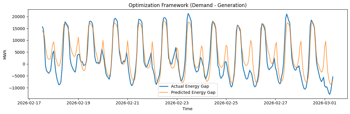
To evaluate how well the framework performed across different seasons, the combined power imbalance analysis was tested over three four-month periods: January–April, May–August, and September–December. Performance metrics were calculated separately for each period. When the demand and renewable generation forecasts were combined, R² decreased from 0.835 and 0.836 for the individual models to 0.71 for the forecasted residuals. This decrease is expected when errors from two independently predicted quantities are carried into a combined calculation and represents a slight increase in unpredictability over time rather than a failure of either model.  As shown in Figure 7, the analysis of forecasted residuals successfully reproduces the timing and direction of most surplus and deficit cycles, despite the compounded uncertainty introduced by combining two independent forecasts. The predicted power imbalance curve follows the overall structure of the observed imbalance signal, indicating that the framework retains meaningful operational information even after error propagation from the demand and generation models. Because the power imbalance is computed by subtracting two independent forecasts, error from both the demand and generation models propagates into the final prediction. Notably, the power imbalance model retains the large majority of the independent models’ explanatory power, a substantially smaller drop than is typically expected in multi-stage forecasting systems, suggesting that the demand and generation models’ errors are only mildly compounding rather than reinforcing one another.

The internal baseline further clarifies the importance of temporal structure and exogenous inputs. The Random Forest model with a one-hour window and no ARX structure achieved only R² = 0.31,demonstrating that even if there is an absence of environmental drivers and limited historical context, the predictive capabilities are greatly diminished. By expanding to a 24-hour autoregressive window and incorporating irradiance variables, performance improved to R² = 0.736 in the analysis of forecasted residuals, a 137% increase over the baseline. The significant improvements in performance confirm the importance of utilizing structured temporal models and incorporating environmental factors into accurate renewable energy forecasts.

Although ANN and LSTM models in the literature report higher R² values (approximately 0.82–0.90), these models rely on more complex recurrent architectures and greater computational overhead. Moreover, they were evaluated on different datasets under distinct experimental conditions, preventing direct quantitative comparison. The present framework demonstrates that separating supply and demand into independent autoregressive models can achieve competitive predictive strength while maintaining simplicity, interpretability, and practical deployability — key requirements for operational grid systems.

Discussion

This study demonstrated that carefully engineered autoregressive machine learning models can effectively forecast short-term electricity demand and renewable generation using real-world grid and environmental data. The primary novelty of this work lies in separating supply and demand forecasting into two independent models. Instead of predicting net load as a single aggregated target, the framework forecasts demand and renewable generation separately before combining the predictions to estimate power imbalance. This separation improves interpretability, allows clearer identification of surplus and deficit conditions, and enables more flexible operational decision-making. The two-layer MLP demand model achieved an R² of 0.835, while the Random Forest ARX generation model achieved an R² of 0.836. When the two forecasts were combined to estimate power imbalance, the integrated framework achieved an R² of 0.736. This reduction in performance reflects the compounded uncertainty introduced by combining two independent forecasts.

These results are comparable to those reported in prior renewable forecasting studies. Feedforward neural networks typically achieve R² values between 0.82 and 0.89, while LSTM-based models achieve values between approximately 0.88 and 0.90. Although this proposed framework does not outperform the current state-of-the-art deep learning models in terms of predictive accuracy, it provides a similar and competitive level of accuracy with increased interpretability and reduced computational complexity.

The limitations of direct quantitative comparison of LSTM and ANN models reported in recent literature are due to the fact that each model has been tested under different experimental conditions. The studies use distinct data sets with different time resolution, geographic scope and predictor sets (different environmental predictors and/or historical grid data). Thus, due to these differences in timeline and data characteristics, like how exogenous variables are used vs. only using historical load data, there is no way to directly compare the performance of these models. These methodological discrepancies significantly impact result interpretation, necessitating a focus on the structural and conceptual merits of the proposed autoregressive framework rather than direct metric parity.

Several limitations should also be acknowledged. First, the models were trained and evaluated using California data, so their performance may not directly generalize to regions with different weather patterns, generation portfolios, or grid operating conditions. Applying the framework to other regions would require retraining the models on local historical data and including environmental predictors relevant to that region. Second, the study was limited to a finite time frame. The results could therefore be different if evaluated over longer periods, which would include more seasonal and year-to-year variation. Our preliminary experiments also indicated that increasing the length of the forecast period beyond 24 hours negatively impacted model performance. Thus, there is an inverse relationship between using historical data to provide context for predictions, and the ability to accurately forecast. Despite this limitation, these results demonstrate that using structured autoregressive models will yield high levels of accuracy in predicting future events while being less reliant on highly complex deep learning architectures.

The proposed framework has practical applications for renewable energy providers, grid operators, and energy monitoring agencies. Separating electricity demand and renewable generation into independent forecasting models provides greater operational interpretability than forecasting net load directly. Because each component is modeled independently, grid operators can determine whether forecasted power imbalances are primarily driven by changes in electricity demand, renewable generation, or both. For example, an unexpected reduction in renewable generation caused by cloud cover or changing wind conditions can be distinguished from unusually high electricity demand. This distinction gives operators more information when making decisions about battery dispatch, backup power generation, and renewable curtailment. Environmental variables such as solar irradiance can also be incorporated to account for and monitor changes in renewable generation caused by weather conditions. This improves situational awareness in systems where generation cannot be directly controlled. The proposed framework therefore contributes to more stable, efficient, and data-driven renewable grid management.

Future work will focus on improving model robustness through more systematic hyperparameter optimization and ensemble learning. Rather than relying on manual experimental tuning, structured hyperparameter search methods such as Random Search and Hyperband could more efficiently identify high-performing model configurations. Ensemble approaches that combine predictions from multiple models may further improve forecasting accuracy and predictive stability by reducing the variance associated with individual models. Additional exogenous variables, including expanded weather and atmospheric features, could further improve renewable forecasting accuracy. Finally, the framework could be extended to larger metropolitan regions or nationwide datasets. This would improve its generalizability while allowing region-specific fine-tuning to account for localized grid dynamics.

References

1. U.S. Energy Information Administration (EIA). California curtailed over 2.4 million megawatt-hours (MWh) of renewable energy in 2023 due to midday solar oversupply. [↩]
2. O. Smith, O. Cattell, and E. Farcot. “The effect of renewable energy incorporation on power grid stability and resilience.” Science Advances. Vol. 8, no. 36, 2022. DOI: 10.1126/sciadv.abj6734. [↩]
3. F. J. M. M. Nijsse, J.-F. Mercure, and N. Ameli. “The momentum of the solar energy transition.” Nature Communications. Vol. 14, no. 1, 2023. DOI: 10.1038/s41467-023-41971-7. [↩]
4. M. J. B. Kabeyi and O. A. Olanrewaju. “Sustainable energy transition for renewable and low carbon grid electricity generation and supply.” Frontiers in Energy Research. Vol. 9, 2022. DOI: 10.3389/fenrg.2021.743114. [↩]
5. A. Assaf, H. Haron, and H. N. Abdull Hamed. “A review on neural network based models for short term solar irradiance forecasting.” Applied Sciences. Vol. 13, no. 14, 2023. DOI: 10.3390/app13148332. [↩]
6. Z. Tarek, M. Y. Shams, and A. M. Elshewey. “Wind power prediction based on machine learning and deep learning models.” Computers, Materials & Continua. Vol. 74, no. 1, 2023. DOI: 10.32604/cmc.2023.032533. [↩]
7. Q. Hassan, S. Algburi, and A. Z. Sameen. “A review of hybrid renewable energy systems: Solar and wind-powered solutions: Challenges, opportunities, and policy implications.” Results in Engineering. Vol. 18, 2023. DOI: 10.1016/j.rineng.2023.101621. [↩]
8. G. G. Njema, R. B. O. Ouma, and J. K. Kibet. “A review on the recent advances in battery development and energy storage technologies.” Journal of Renewable Energy. Vol. 2024, 2024. DOI: 10.1155/2024/2329261. [↩]
9. T. Hong, P. Pinson, and Y. Wang. “Energy forecasting: A review and outlook.” IEEE Open Access Journal of Power and Energy. Vol. 7, 2020. DOI: 10.1109/OAJPE.2020.3029979. [↩]
10. N. E. Benti, M. D. Chaka, and A. G. Semie. “Forecasting renewable energy generation with machine learning and deep learning: Current advances and future prospects.” Sustainability. Vol. 15, no. 9, 2023. DOI: 10.3390/su15097087. [↩]
11. R. Ahmed, V. Sreeram, and Y. Mishra. “A review and evaluation of the state-of-the-art in PV solar power forecasting: Techniques and optimization.” Renewable and Sustainable Energy Reviews. Vol. 136, 2020. DOI: 10.1016/j.rser.2020.109792. [↩]
12. P. Kumari and D. Toshniwal. “Extreme gradient boosting and deep neural network based ensemble learning approach to forecast hourly solar irradiance.” Journal of Cleaner Production. Vol. 273, 2020. DOI: 10.1016/j.jclepro.2020.123285. [↩]
13. S. Hanifi, A. Cammarono, and H. Zare-Behtash. “Advanced hyperparameter optimization of deep learning models for wind power prediction.” Renewable Energy. Vol. 208, 2023. DOI: 10.1016/j.renene.2023.119700. [↩]
14. Z. Lin, X. Liu, and M. Collu. “Wind power prediction based on high-frequency SCADA data along with isolation forest and deep learning neural networks.” International Journal of Electrical Power & Energy Systems. Vol. 123, 2020. DOI: 10.1016/j.ijepes.2020.105835. [↩]
15. D. Markovics and M. J. Mayer. “Comparison of machine learning methods for photovoltaic power forecasting based on numerical weather prediction.” Renewable and Sustainable Energy Reviews. Vol. 170, 2022. DOI: 10.1016/j.rser.2022.112364. [↩]
16. A. Zeng, M. Chen, and L. Zhang. “Are transformers effective for time series forecasting?” Proceedings of the AAAI Conference on Artificial Intelligence. Vol. 37, no. 9, 2023. DOI: 10.1609/aaai.v37i9.26317. [↩]
17. Z. Wu, S. Pan, and G. Long. “Connecting the dots: Multivariate time series forecasting with graph neural networks.” Proceedings of the 26th ACM SIGKDD International Conference on Knowledge Discovery & Data Mining, 2020. DOI: 10.1145/3394486.3403118. [↩]
18. H. Zhou, S. Zhang, and J. Peng. “Informer: Beyond efficient transformer for long sequence time-series forecasting.” Proceedings of the AAAI Conference on Artificial Intelligence. Vol. 35, no. 12, 2021. DOI: 10.1609/aaai.v35i12.17325. [↩]
19. I. K. Nti, M. Teimeh, and O. Nyarko-Boateng. “Electricity load forecasting: A systematic review.” Journal of Electrical Systems and Information Technology. Vol. 7, 2020. DOI: 10.1186/s43067-020-00021-8. [↩]
20. I. Shah, H. Iftikhar, and S. Ali. “Modeling and forecasting electricity demand and prices: A comparison of alternative approaches.” Journal of Mathematics. Vol. 2022, 2022. DOI: 10.1155/2022/3581037. [↩]
21. W. Guo, L. Che, and M. Shahidehpour. “Machine-learning based methods in short-term load forecasting.” The Electricity Journal. Vol. 33, no. 10, 2020. DOI: 10.1016/j.tej.2020.106884. [↩]
22. B. Ibrahim, L. Rabelo, and E. Gutiérrez-Franco. “Machine learning for short-term load forecasting in smart grids.” Energies. Vol. 15, no. 21, 2022. DOI: 10.3390/en15218079. [↩]
23. H. Habbak, M. Mahmoud, and K. Metwally. “Load forecasting techniques and their applications in smart grids.” Energies. Vol. 16, no. 3, 2023. DOI: 10.3390/en16031480. [↩]
24. J. M. Aguiar-Pérez and M. A. Pérez-Juárez. “An insight of deep learning based demand forecasting in smart grids.” Sensors. Vol. 23, no. 3, 2023. DOI: 10.3390/s23031467. [↩]
25. I. Antonopoulos, V. Robu, and B. Couraud. “Artificial intelligence and machine learning approaches to energy demand-side response: A systematic review.” Renewable and Sustainable Energy Reviews. Vol. 133, 2020. DOI: 10.1016/j.rser.2020.109899. [↩]
26. F. R. Alharbi and D. Csala. “A seasonal autoregressive integrated moving average with exogenous factors (SARIMAX) forecasting model-based time series approach.” Inventions. Vol. 7, no. 4, 2022. DOI: 10.3390/inventions7040094. [↩]
27. J. Browell and M. Fasiolo. “Probabilistic forecasting of regional net-load with conditional extremes and gridded NWP.” IEEE Transactions on Smart Grid. Vol. 12, no. 5, 2021. DOI: 10.1109/TSG.2021.3107159. [↩]
28. A. Faustine and L. Pereira. “FPSeq2Q: Fully parameterized sequence to quantile regression for net-load forecasting with uncertainty estimates.” IEEE Transactions on Smart Grid. Vol. 13, no. 4, 2022. DOI: 10.1109/TSG.2022.3148699. [↩]
29. H. Hadian and F. Naderkhani. “Deep learning-based models for wind and solar curtailment forecasting.” Proceedings of the International Conference of Energy Harvesting, Storage, and Transfer, 2023. DOI: 10.11159/EHST23.120. [↩]
30. Z. Liu and Y. Du. “Evolution towards dispatchable PV using forecasting, storage, and curtailment: A review.” Electric Power Systems Research. Vol. 222, 2023. DOI: 10.1016/j.epsr.2023.109554. [↩]
31. T. Chen, Y. Jin, and H. Lv. “Applications of lithium-ion batteries in grid-scale energy storage systems.” Transactions of Tianjin University. Vol. 26, 2020. DOI: 10.1007/s12209-020-00236-. [↩]
32. GridStatus. CAISO Standardized Hourly Dataset. Available at: https://www.gridstatus.io/datasets/caiso_standardized_hourly. [↩]
33. SolarAnywhere Historical Time-Series Data Documentation. Available at: https://www.solaranywhere.com/support/historical-data/time-series/. [↩]
34. Forecasting time series with scikit-learn. Available at: https://cienciadedatos.net/documentos/py27-time-series-forecasting-python-scikitlearn.html. [↩]
35. Y. Jiang, Y. Li, and Y. Chen. “Interpretable Short-Term Load Forecasting via Multi-Scale Temporal Decomposition.” Electric Power Systems Research. Vol. 235, 2024. Article 110781. [↩]
36. P. A. Gbadega, Y. Sun, and O. A. Balogun. “Optimized energy management in grid-connected microgrids leveraging K-means clustering algorithm and artificial neural network models.” Energy Conversion and Management. Vol. 336, 2025. Article 119868. [↩]
37. A. Showole and M. S. Afaqui. “Optimization of renewable energy management using machine learning and genetic algorithms.” Energy Storage and Saving, 2026. [↩]