Forecasting and Validating Delhi’s Air Quality Index Using Machine Learning: A Multi-Model Approach with Real-World Verification

Abstract

Delhi experiences high air pollution, especially during winter when AQI values often reach hazardous levels. This study used 1,461 daily observations from the DTU campus monitoring station collected between 2021 and 2024. It examined which pollutants were most strongly related to AQI and tested whether machine learning models could predict next-day AQI using previous pollutant values. Three regression models were used: Linear Regression, Random Forest, and XGBoost. Lagged pollutant features were used to avoid target leakage from same-day values. After hyperparameter tuning, XGBoost performed best, with a test RMSE of 72.61 and an R² of 0.499. SHAP analysis showed that lagged PM2.5 and PM10 values had the strongest influence on the predictions. A CPCB-based benchmark was also used to compare the machine learning results with AQI calculated using the official CPCB method. Prophet was trained on data from 2021 to 2024 and validated using AQI values calculated from pollutant measurements recorded at DTU between October 13 and November 30, 2025. Prophet had a validation RMSE of 99.83 and correctly identified 69.39% of days with an AQI above 400. Its performance was lower when identifying days with AQI above 300. The results show that lagged pollutant data can provide useful information for AQI forecasting, but accurate next-day predictions remain difficult when only these features are used. The use of one monitoring station and the absence of weather-related variables were the main limitations.

Keywords: Air Pollution Forecasting, Air Quality Index, Data Science, Machine Learning, XGBoost, Random Forest, Prophet, SHAP, Time Series Forecasting

Introduction

Delhi’s AQI, especially during winter has been a matter of serious concern since 2016¹. Every winter Delhi’s AQI rises to the point where AQI falls in severe category. This affects hundreds of thousands of Delhi’s residents.

According to CPCB, AQI is calculated from six pollutants¹. These are PM10, PM2.5, nitrogen dioxide, sulfur dioxide, carbon monoxide, and ozone. Though 6 pollutants are used in calculation of AQI, there are only 2 pollutants which cause sharp rise and fall in AQI. They are particulate matters (PM10 and PM2.5). In this study, PM10 was more of a major drive in AQI than PM2.5. However, PM2.5 is more biologically harmful because it is much smaller and can go deep into the lungs and into the bloodstream, increasing the risk of heart disease, lung cancer, and strokes over time². Delhi’s annual average concentration of PM2.5 in 2023 was around 88 µg/m³, or about 17 times the WHO’s recommended limit³.

Besides these 6 pollutants, nature plays a role too in Delhi’s high AQI. Winter temperature inversions trap pollutants near the ground^4,5. Delhi’s location in the Indo-Gangetic Plain limits air circulation⁶. Vehicle emissions, construction dust, and industrial activity add to the pollution load⁶. Crop residue burning in nearby states and Diwali emissions cause further spikes each year during winter^7,6.

This annual trend was disturbed by lockdowns throughout the world due to COVID-19. During lockdowns, use of vehicles and industrial activities decreased significantly which caused AQI to fall^8,9. After 2021, restrictions were lifted which caused AQI to rise again as everyday-life came back to its pre-pandemic routine.

Machine learning has become an important tool for tasks related to forecasting and research in different domains. Air quality/Environment being one of them as they contain complex, non-linear interactions that traditional statistical models handle poorly^10,11. Ensemble methods like Random Forest and XGBoost are well suited to identifying these patterns^12,13. Time series models like Prophet can capture seasonal cycles and long-term trends¹⁴. A number of studies have applied these methods to Delhi’s air quality and found that machine learning models generally outperform traditional approaches, though few validate predictions against actual future observations^15,16,17,18. For example, Gupta et al. (2025) and Masood & Ahmad (2023) have demonstrated strong model performance on historical Delhi data but do not validate forecasts against future observations^15,18. Some also use pre-2021 data but do not capture the post-pandemic pollution rebound^19,18.

This study addresses both gaps listed. First, it compares three regression models trained on lagged pollutant features to forecast next-day AQI. Second, it validates forecast produced by prophet against real-world observations from the DTU monitoring station from October 2025 to November 2025²⁰. The major hypotheses were that PM2.5 and PM10 would show stronger correlations with AQI, with PM10 expected to exceed a Pearson correlation of 0.8, and that ensemble models would outperform Linear Regression in R², RMSE, MAE and MAPE, with XGBoost expected to lead due to its sequential boosting framework.

The dataset used in this study was obtained from kaggle. It consists of 1,461 daily observations from January 2021 through December 2024²¹. Meteorological variables were unavailable and therefore excluded, which limits predictive accuracy but does not negatively affect meaningful seasonal forecasting over the study period.

Methods

Research Design

This study was conducted based on publicly available historical air-quality data. No experiments were conducted, and no human participants were involved. The pollutant data were used to train machine-learning models for next-day AQI prediction and a Prophet model for long-term AQI forecasting.

Data Collection

Daily air quality data from Delhi’s DTU campus from January 2021 through December 2024 was obtained from a publicly available Kaggle dataset²¹. The dataset contains 1,461 daily observations of PM2.5, PM10, NO2, SO2, CO, and Ozone, alongside corresponding AQI values and calendar features including holiday counts and weekday indicators. There were no missing values in the dataset. The data was loaded and manipulated using python’s pandas library. The data was grouped in months and years to analyze seasonal patterns. Meteorological variables such as wind-speed, temperature and humidity were not available in the dataset therefore were not used anywhere throughout the study. Including them would have likely improved forecasting accuracy, as conditions such as temperature inversion plays role in extreme pollution episodes^4,5.

Feature Engineering and Target Variable

Input features were prepared using pollutant measurements from one, two, three, and seven days before the prediction date. Same-day pollutant values were not used because they are directly involved in calculating AQI under the CPCB framework. The lagged values created 24 input features in total. The lags of one, two, and three days were used to capture recent pollution patterns. The seven-day lag was included to account for possible weekly changes in traffic and industrial activity. Creating these lagged features removed the first seven observations because earlier data were unavailable, reducing the dataset from 1,461 to 1,454 observations. AQI was used as the target variable, with previous pollutant measurements used to predict the next day’s AQI.

PM2.5 and PM10 concentrations were measured in micrograms per cubic meter. NO2, SO2, and O3 were measured in micrograms per cubic meter or parts per billion, depending on the sensor, while CO was measured in milligrams per cubic meter. AQI is a dimensionless quantity. It is calculated by finding a separate sub-index for each pollutant and using the highest sub-index as the final AQI value. Therefore, the pollutant with the highest sub-index has the greatest effect on the overall AQI.

Exploratory Data Analysis

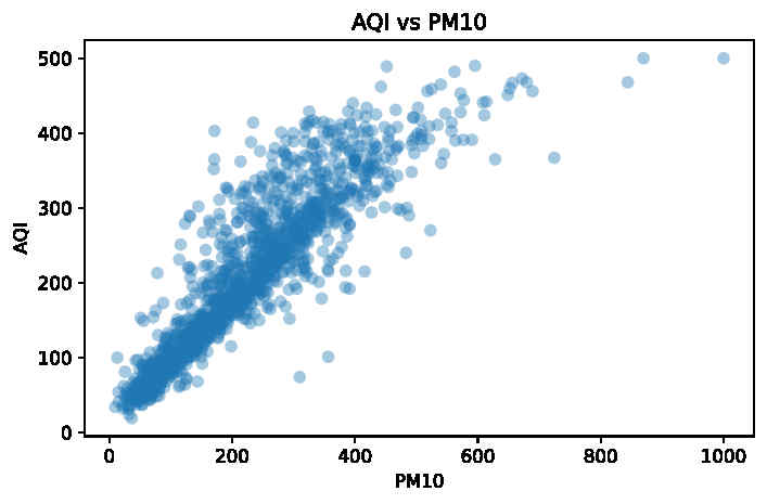
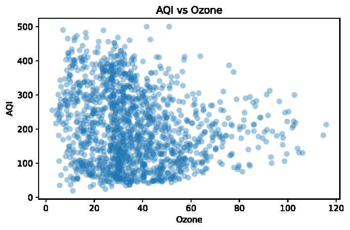
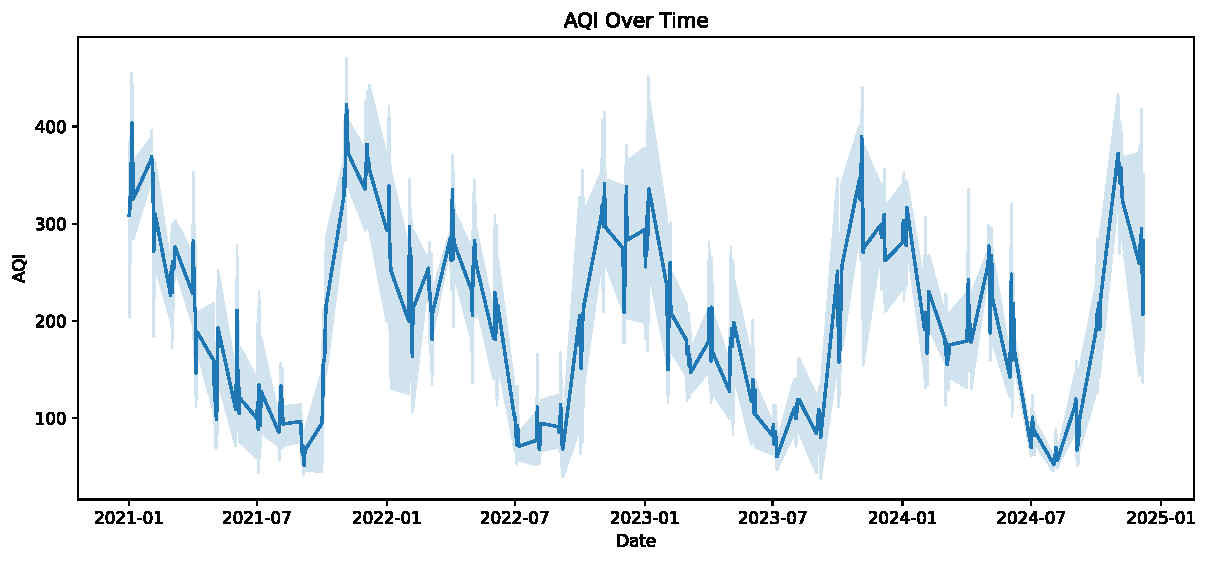
Pearson correlation coefficients were calculated to measure the strength and direction of the relationship between each pollutant and AQI. Scatter plots were created to visualize these relationships, while a correlation heatmap showed the relationships among all pollutants and AQI. The data were also grouped by month, and a line plot was used to examine AQI trends over the study period.

Variance Inflation Factors (VIF) were calculated for the original six pollutant features and the 24 lagged features to check for multicollinearity. The lagged features showed high multicollinearity, with the highest VIF reaching 14.6 for a PM10 lag feature. This was expected because pollutant concentrations from nearby days are often related. Since Random Forest and XGBoost are tree-based models, multicollinearity was not expected to significantly affect their predictions. However, the Linear Regression results were interpreted with caution.

Seasonal decomposition was applied to the AQI data to separate long-term trends, seasonal patterns, and unexplained variation. A Kruskal–Wallis test was also performed to determine whether AQI differed significantly across months.

Data Splitting Strategy

The dataset was split chronologically, with the first 80% used for training and the remaining 20% used for testing. This ensured that the models were tested on data from a later period than the data used for training. Five-fold TimeSeriesSplit cross-validation was used to maintain the chronological order of the data, with each validation set coming after its corresponding training set. The same TimeSeriesSplit method was used during hyperparameter tuning with RandomizedSearchCV. The original 80/20 split was retained for the final evaluation, while cross-validation was used only for model tuning and checking the consistency of the results.

Linear Regression

Linear Regression was implemented as the baseline model using scikit-learn’s LinearRegression class²². The model fits a linear equation of the form:

Here, t represents the day for which AQI is predicted, while t−1, t−2, t−3, and t−7 represent one, two, three, and seven days earlier. Each coefficient shows how its corresponding lagged pollutant value affects the predicted AQI.

Linear Regression has no meaningful hyperparameters to tune, so it was trained once on the training set and evaluated directly on the test set. It serves as a reference point for measuring the improvement the ensemble models achieve by capturing non-linear relationships.

Random Forest Regressor

Random Forest was implemented using scikit-learn’s RandomForestRegressor class. The model constructs a large number of decision trees, each trained on a bootstrap sample of the training data and a random subset of features at each split node. This combination of data and feature sampling introduces diversity among the trees, reducing overfitting and improving generalization. The final prediction is the average across all individual trees¹².

XGBoost Regressor

XGBoost was implemented using the XGBRegressor class from the XGBoost library. Unlike Random Forest, which builds multiple trees independently and combines their predictions, XGBoost builds trees one after another. Each new tree attempts to correct the errors made by the previous trees. XGBoost also uses L1 and L2 regularization to reduce overfitting and improve model performance¹³.

A rule-based CPCB benchmark was also created using the official sub-index formulas for PM2.5 and PM10. The highest sub-index was used as the predicted AQI, following the CPCB method. This benchmark was used as a reference to compare the machine-learning models with AQI calculated from same-day pollutant concentrations.

Hyperparameter Tuning

For both Random Forest and XGBoost, hyperparameter tuning was performed using RandomizedSearchCV with five-fold TimeSeriesSplit cross-validation, evaluating 20 random combinations per model. Linear Regression was excluded from tuning as it has no meaningful hyperparameters to optimize. Table 1 summarizes the hyperparameters tested and the optimal values identified for each model.

Hyperparameter	Search Space (Random Forest)	Search Space (XGBoost)	Best parameter (Random Forest)	Best parameter (XGBoost)
n_estimators	100, 200, 300, 400, 500	200, 400, 600	100	400
max_depth	None, 10, 20, 30, 40	3, 5, 7, 9	None	3
min_samples_split	2, 5, 10	—	5	—
learning_rate	—	0.01, 0.05, 0.1	—	0.01
subsample	—	0.7, 0.8, 1.0	—	0.7
colsample_bytree	—	0.7, 0.9, 1.0	—	1.0

Model Evaluation Metrics

Four evaluation metrics were used to evaluate the prediction results: Root Mean Squared Error (RMSE), Mean Absolute Error (MAE), R², and Mean Absolute Percentage Error (MAPE).

The Root Mean Squared Error (RMSE) is calculated as the square root of the average of the squared difference between the predicted and actual AQI values. Because the errors are squared, larger prediction errors have a greater impact on the final RMSE. A lower RMSE thus indicates that the predicted AQI values were closer, on average, to the actual values.

The Mean Absolute Error is the average of the differences between the predicted AQI and the actual AQI, regardless of whether the prediction is higher or lower than the actual. It gives the average prediction error in AQI units directly. Lower MAE indicates the predicted AQI values are closer to the observed values.

The R² score indicates the percentage of the variation in AQI explained by the input data. An R² value of 1.0 indicates a perfect fit, and 0 indicates the predictive results that were no better than the average AQI value. The higher the R², the more of the variation in AQI was explained by the predictions.

The Mean Absolute Percentage Error shows the average error of the predictions as a percentage of the actual AQI value. Unlike RMSE and MAE, it expresses the error as a percentage, not in AQI units. This gives a better idea of how large the prediction error is relative to the actual AQI.

SHAP Analysis

SHAP analysis was applied to the tuned XGBoost model to interpret how each lagged pollutant feature influenced individual AQI predictions¹⁰. TreeSHAP was used because it computes exact SHAP values efficiently for tree-based models²³. SHAP values quantify the contribution of each feature to a prediction while considering interactions among features. Two plots were generated from the analysis: a bar plot showing the mean absolute SHAP value of each feature across the test set, and a beeswarm plot showing the distribution of SHAP values for each feature, with color indicating whether the corresponding feature value was relatively high or low.

Time Series Forecasting with Prophet

Prophet was selected to forecast AQI over a longer period because the Delhi AQI data showed a clear yearly pattern, with major pollution peaks during late autumn. The trend also changed during the period following COVID-19¹⁴. Prophet was used because it can account for both long-term trends and seasonal changes, while allowing the trend to shift over time^24,14. Its forecasts were evaluated alongside those from a seasonal naïve model and a SARIMA model²⁵.

The seasonal naïve model predicted AQI using the value recorded on the same date one year earlier. SARIMA was fitted using the auto_arima function from the pmdarima library with a seasonal period of seven days. The same chronological 80/20 train-test split was used for Prophet and both baseline models²⁶.

Prophet was set up with linear growth and yearly seasonality. Weekly and daily seasonal patterns were turned off because they were not clearly visible in the data. The changepoint prior scale was set to 0.05 to allow changes in the trend without making the model too sensitive to small changes in AQI.

After the initial evaluation, Prophet was trained using the full dataset from 2021 to 2024. It was then used to generate daily AQI forecasts through 2026. The uncertainty intervals became wider as the forecast moved further into the future.

The forecasts for October and November 2025 were checked against AQI values calculated from pollutant measurements recorded at the DTU monitoring station. CO measurements were unavailable, so AQI was calculated using the official CPCB sub-index formulas for the other five pollutants. The highest sub-index was taken as the final AQI value. Eleven days with missing pollutant measurements were removed, leaving 49 days for validation.

Ethical Considerations

The dataset used in this study is publicly available on Kaggle and is based on air-quality records from the Central Pollution Control Board of India. The dataset was anonymized and did not contain any personal information. No human participants were involved. The dataset was available for research and educational use. The code used in this study was uploaded to GitHub to make the analysis easier to check and reproduce.

Code Availability

To support reproducibility and methodological transparency, the complete analysis pipeline, including data preprocessing, machine learning model training, hyperparameter tuning, SHAP analysis, and Prophet forecasting, is publicly available at https://github.com/Shaurya-git-bit/Delhi-AQI-Time-Series-Forecasting-with-Prophet.

Results

Forecasting Baseline Comparison

Before comparing Prophet forecasts against the 2025 observations, it was tested on the test set with the other two baseline models which were seasonal naïve model and SARIMA. The seasonal naïve model had RMSE equal to 88.48 and MAE equal to 67.86, while SARIMA had RMSE of 102.96 and MAE of 85.62. Prophet was validated on the measurements of pollutants at DTU through which AQI was calculated from October 13, 2025 to November 30, 2025²⁰. It had a validation RMSE of 99.83 and MAE of 73.3. Since the baseline models were validated on a different set than Prophet, comparing the absolute errors is unfair. The Prophet model correctly predicted 69.39% of days with an AQI over 400 and 55.10% of days with an AQI over 300.

Forecast Validation against Real 2025 Observations

The forecasts produced by Prophet were validated against AQI values calculated from pollutant measurements recorded at the DTU campus monitoring station between October 13 and November 30, 2025. Since CO measurements were unavailable, AQI was calculated using the other five pollutants and the official CPCB sub-index equations. Eleven days with incomplete pollutant data were removed, leaving 49 observations for evaluation.

Prophet had a validation RMSE of 99.83 and MAE of 73.3. It correctly predicted 69.39% of days with AQI over 400, and 55.10% of days over 300. The seasonal naive model had RMSE of 88.48 and MAE of 67.86. SARIMA had RMSE of 102.96 and MAE of 85.62. These aren’t directly comparable since Prophet was tested on a different set. Therefore their RMSE values should be interpreted separately.

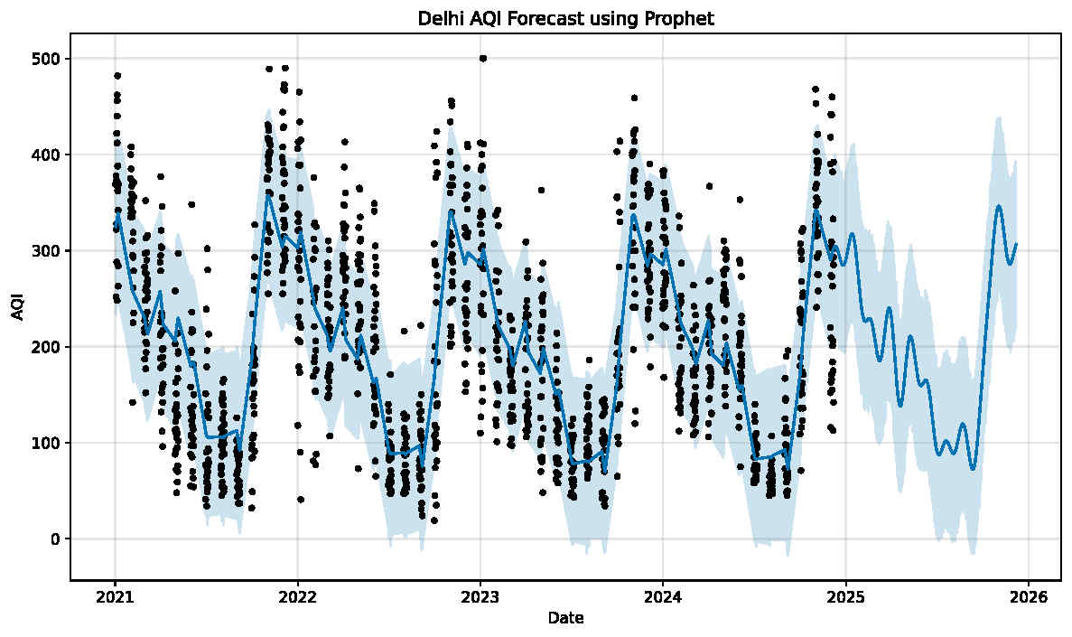
Figure 1 shows the Prophet forecast alongside actual AQI observations from 2021 through 2026. Black dots are the daily AQI values recorded at the DTU monitoring station. The blue line is Prophet’s fitted and forecasted AQI, and the shaded blue band is the uncertainty interval. The band widens as the forecast extends further into the future.

The plot shows Delhi’s seasonal pattern: AQI peaks each winter and declines during the monsoon months, repeating across all four years of training data. The uncertainty interval is larger during winter peaks than during monsoon months. Beyond 2025, where no observed data exist, the interval keeps expanding as the forecast moves further out.

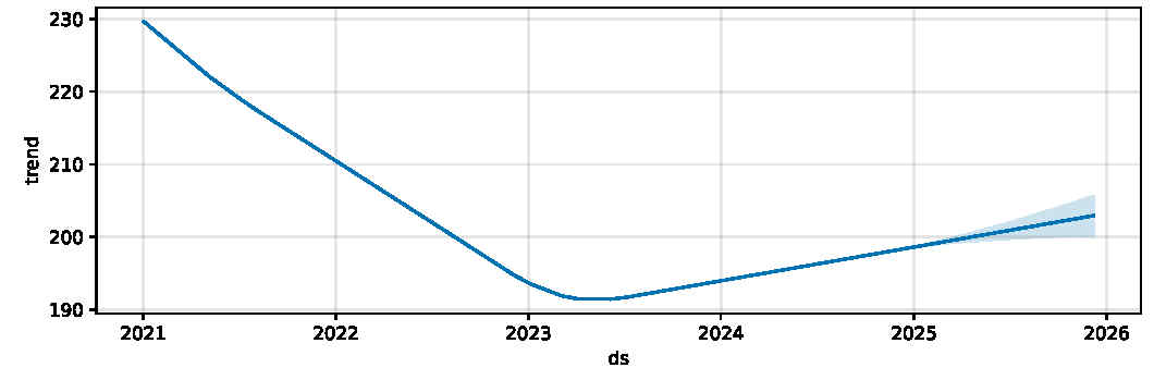
The trend component shows the long-term direction of Delhi’s AQI after removing seasonal and random variation. AQI declined from early 2021 to mid-2023, possibly due to reduced economic and vehicular activity during the post-pandemic recovery. It rose again through 2024 as activity returned to normal.

Correlation between Pollutants and AQI

Correlation with AQI (r = 0.90) indicated a strong positive correlation for PM10 with a clear positive trend. PM2.5 was also found to be highly correlated with AQI (r = 0.82), but the variation in values was much larger for higher concentrations. CO was moderately related to AQI (r = 0.71) other pollutants showed lower correlations, with weak correlations for NO2, SO2 and O3 with AQI. For O3 the correlation was scattered without any obvious trend. Due to the limited information provided by the correlation metric, a more detailed analysis was performed using the SHAP approach.

VIF analysis was performed to determine the extent of multicollinearity among the six features of pollutants. The highest VIF scores were for PM10 (9.44), followed by CO (7.75) and PM2.5 (6.88). The VIF values of NO2, SO2 and O3 were less than 3. PM10 and PM2.5 had relatively high VIF scores, but both were retained because of their overall importance.

The 24 lagged features showed similar pattern with the highest VIF score of 14.59 for PM10_lag7. The Linear Regression results should be interpreted with caution due to the expected degree of collinearity between lagged features.

Seasonal Patterns in AQI

The analysis of the monthly AQI distribution showed a seasonal pattern during the four years. The highest AQI levels were typically observed in November, December and January, with median values of 300 to 400. The lowest AQI values were found in July, August and September with median values below 150 and little variance between months. The AQI for the months of February, March, April and September, October was relatively low in the respective months.

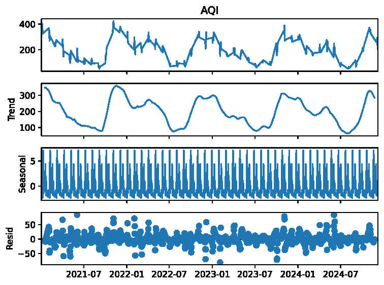
The decomposition method was used to decompose the original AQI series into trend, seasonal and residual components. The graph of the three series is below. The trend component showed several increases and decreases throughout the study period from 2021 to 2024. The seasonal component showed seasonal variation in AQI with increases in winter months and decreases in monsoon season. This pattern was the same for all four years of the analysis. The residual component represented short term variations in AQI and values were mostly clumped around zero, with few large outliers during severe pollution episodes like Diwali festival and stubble burning events.

A Kruskal-Wallis test was conducted to determine whether the distribution of AQI was equal across all months. The test confirmed that the distribution was not equal (H = 886.36, p < 0.001).

Machine Learning Model Performance before Tuning

Three models were trained on the first 80% of the chronological data using 24 predictors of lagged values of pollutants and tested on the remaining 20%. Before hyperparameter optimization, Linear Regression outperformed with an RMSE of 70.52, MAE of 56.55, R² of 0.527, and MAPE of 41.84%. Random Forest followed up with an RMSE of 74.89, MAE of 61.60, R² of 0.467, and MAPE of 50.60%. XGBoost had the lowest baseline performance with RMSE of 81.59, MAE of 66.67, R² of 0.367, MAPE of 55.27%

Linear Regression outperformed both ensemble models before tuning. This came out to be unexpected. Multicollinearity among the lagged features is one possible cause, since linear models are generally more sensitive to correlated predictors than tree-based ones. It is not the only reason, and this assumption should be explored further in later sections; thus, it is included in the Discussion.

Model	RMSE	MAE	R²	MAPE
Linear Regression	70.52	56.55	0.527	41.84%
Random Forest	74.89	61.60	0.467	50.60%
XGBoost	81.59	66.67	0.367	55.27%

Machine Learning Model Performance after Tuning

The use of RandomizedSearchCV and TimeSeriesSplit cross-validation for hyperparameter tuning resulted in XGBoost achieving an RMSE of 72.61, an MAE of 59.93, an R² of 0.499, and a MAPE of 46.91%. Random Forest showed similar performance, with an RMSE of 73.75, an MAE of 60.29, an R² of 0.483, and a MAPE of 48.63%. Hyperparameter tuning improved the performance of XGBoost, but the difference between the two tuned models remained small. Although Linear Regression was not tuned, it achieved an R² of 0.527 on the test set. This may be related to the strong multicollinearity among the lagged features, although this explanation cannot be confirmed from the present analysis.

The cross-validation results across all three approaches yielded an average R² of about 0.33 to 0.36. Random Forest had the highest mean of R² of 0.3555 with the lowest variance (standard deviation) of 0.0909. Therefore, it was more stable in its results on the 10 folds of the cross validation. XGBoost had a slightly lower mean R² of 0.3446 and standard deviation of 0.1040. The Linear Regression had the lowest mean R² of 0.3342 and highest standard deviation of 0.1740.

Model (Tuned)	RMSE	MAE	R²	MAPE
Random Forest	73.75	60.29	0.483	48.63%
XGBoost	72.61	59.93	0.499	46.91%

The CPCB-based model, which effectively used the same-day pollutant values to estimate AQI, had an RMSE of 55.74, an MAE of 28.65, and an R² of 0.732. It outperformed the lag-based machine learning models, which is expected since it used the same-day pollutant values, while the latter used the lagged values to predict AQI. Thus, predicting AQI based on previous days’ pollutant values is a more challenging task than estimating it from the same-day values.

Model	Mean R² (± Std)	Mean RMSE (± Std)	Mean MAE (± Std)
Linear Regression	0.3342 ± 0.1740	82.57 ± 15.03	64.04 ± 11.00
Random Forest	0.3555 ± 0.0909	81.25 ± 6.89	64.36 ± 6.89
XGBoost	0.3446 ± 0.1040	81.85 ± 8.09	64.93 ± 7.27

The cross-validation results for the three approaches were relatively similar, with mean R² values ranging from 0.33 to 0.36. This result indicated that the problem of predicting the next day AQI from lagged pollutant values was difficult and all three approaches achieved only moderate predictive performance. Random Forest was the best performing model of the three, with a mean R² of 0.3555 and the lowest variance across folds (standard deviation of 0.0909). XGBoost had a mean R² of 0.3446 and standard deviation of 0.1040. The Linear Regression had the least mean R² of 0.3342 with a standard deviation of 0.1740. It was therefore the least consistent in the results from the 10 folds of the cross-validation.

 SHAP Analysis of the XGBoost Model

The SHAP analysis was used to assess the contribution of each lagged pollutant feature to the final AQI prediction. For the tuned XGBoost model, the mean absolute SHAP values were as follows: PM2.5_lag1 = 11.66, PM2.5_lag3 = 11.39, PM10_lag1 = 10.01, PM2.5_lag2 = 7.41, PM10_lag2 = 6.87, PM10_lag3 = 6.73, PM2.5_lag7 = 4.87, NO2_lag1 = 4.49, SO2_lag3 = 3.64, PM10_lag7 = 3.07. The lag features of PM2.5 and PM10 had the highest contribution to the model, with the exception of PM10_lag7. The lag features of gaseous pollutants had a relatively low contribution to the model. For example, PM2.5_lag1 indicates the value of PM2.5 concentration from the previous day. Similarly, lag2, lag3, and lag7 indicate the value of the pollutant concentration from two, three, and seven days ago, respectively.

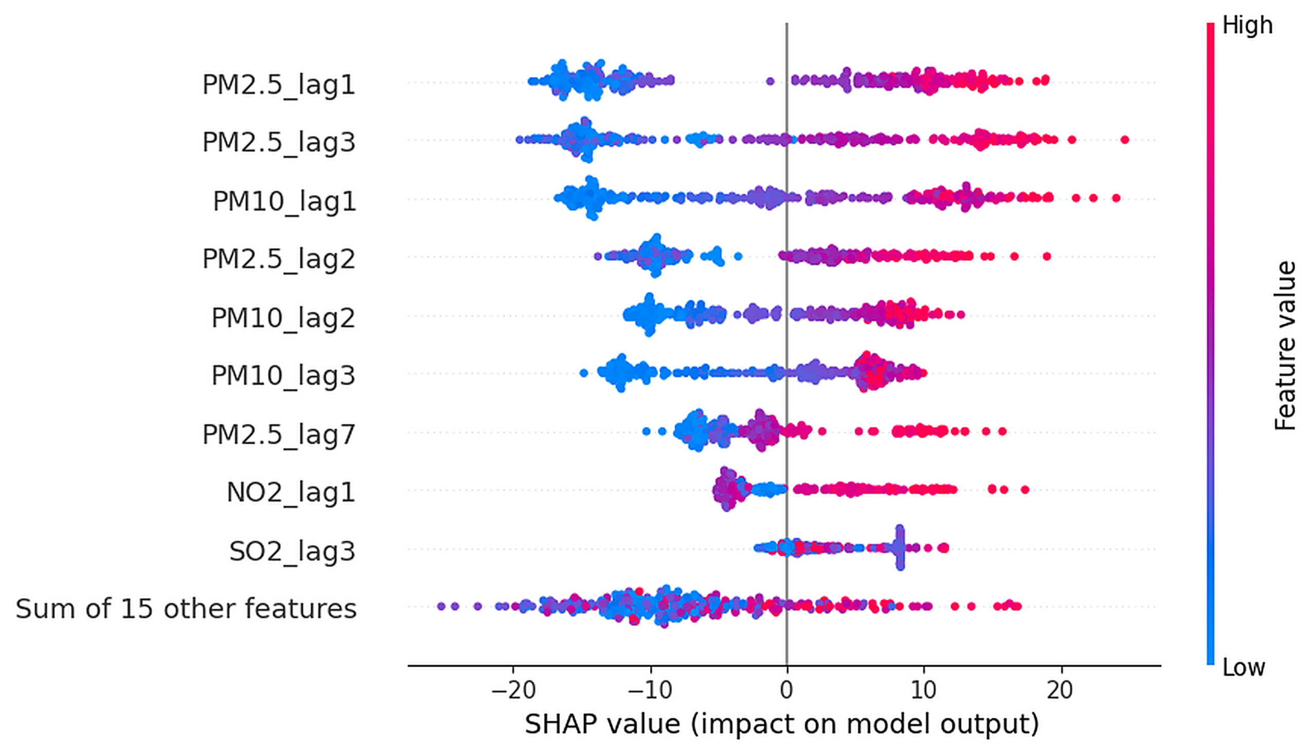
The figure shows how previously recorded pollutant values affected AQI predictions made by the XGBoost model. PM2.5_lag1 had the strongest effect, followed by PM2.5_lag3 and PM10_lag1. The red points represent higher pollutant values and are mostly found on the right side of the plot. This shows that higher pollutant levels generally increased the predicted AQI. The blue points represent lower pollutant values and are mostly found on the left side, meaning that lower values generally decreased the predicted AQI. The one-day and three-day lag features had a stronger effect than the seven-day lag features. This suggests that the model relied more on recent pollutant data than on older observations.

Discussion

After hyperparameter tuning, XGBoost showed the best overall performance, although its advantage over Random Forest was small. Both models performed below the CPCB benchmark. PM2.5 and PM10 values from previous days were the most important predictors of next-day AQI.

Lagged features were used to avoid target leakage. Under the CPCB framework, AQI is calculated using pollutant concentrations from the same day. Using those same-day values as model inputs would therefore reconstruct AQI rather than predict it in advance. The CPCB benchmark achieved a higher R² of 0.732 because it used the same-day pollutant values, while the machine-learning models used earlier observations. The cross-validation results showed mean R² values between 0.33 and 0.36. This suggests that the lagged models provided some forecasting value, although their performance remained limited.

Before and even after tuning, Linear Regression performed better than the ensemble models which was unexpected. This may be because the lagged features had high multicollinearity. The VIF values for the PM10 lag features ranged from 13.93 to 14.59, indicating high multicollinearity which may have affected model performance. The strong correlations between PM2.5, PM10, and AQI may also have favored Linear Regression, as it can capture these linear relationships effectively. Another possible reason is that the dataset had fewer than 1,500 observations with only 24 features, which may not have been enough for the tree-based models to learn strong patterns. These are possible explanations, not confirmed causes.

Tuning improved XGBoost the most. Its RMSE decreased from 81.59 to 72.61, while its R² increased from 0.367 to 0.499. Random Forest also improved but less than XGBoost. After tuning both the ensemble models, all three models still had fairly similar performance. This suggests that the available predictor variables may have limited performance more than the choice of model. Absence of meteorological variables such as wind speed, temperature, humidity, rainfall, and boundary layer height might have contributed to this modest improvement. Previous studies who used these variables reported better model performance though it is not completely known due to small size of dataset²⁷.

SHAP results supported the earlier correlation analysis. PM2.5 and PM10 values from one and three days earlier had the strongest effect on AQI predictions, while gaseous pollutants had much smaller effects. This may be related to particulate pollution remaining in the air for several days, especially during stagnant winter conditions⁴. It must be noted that SHAP values describe how the model fitted the features and not about the physical processes that actually determine AQI. Thus, the two aspects can differ, and the conducted analysis cannot tell whether there is a real cause-and-effect relationship or a mere statistical correlation^28,23.

The classification of episodes by the Prophet model was inconsistent, and it seems that this has more to do with the characteristics of the model itself than the data it worked with. Extreme events, referring to AQI values above 400, occur during a distinct seasonal period, which remains consistent each year. On the contrary, episodes with moderate to high AQI are influenced by factors such as weather and emissions, which were not included in the Prophet model, leading to weaker predictions within these ranges. The model was also used to generate forecasts over a long period. As the forecast moved further into the future, uncertainty increased, which may have affected its accuracy.

The decreasing trend in AQI from 2021 to mid-2023, followed by an increase in 2024, may be linked to the return of transport and industry after the pandemic. However, this point was not tested in detail in the research and should be considered a plausible explanation rather than a proven cause.

Future studies may be able to use multiple monitoring sites across Delhi, allowing for a more accurate assessment of pollution in different areas¹⁹. Including meteorological factors may make forecasts more accurate, especially during moderate-to-severe pollution episodes that are difficult to classify²⁷. Other modeling methods, such as Long Short-Term Memory (LSTM) networks, could also be tested for longer-range forecasting. Forecasting models could also be combined with emissions data or source-apportionment data to better connect prediction results with the sources of pollution^7,26.

Limitations

The study had four main limitations:

First, the dataset used in this study contains records from a single monitoring station at DTU, so the findings may not represent pollution levels across all of Delhi.

Second, meteorological variables were not included throughout the study which likely limited models’ performance.

Third, the analysis used publicly available data from CPCB monitoring stations. While they presumably reflect actual air quality, the calibration of the sensors cannot be verified.

Fourth, during the October to November 2025 validation period, CO data were unavailable. Therefore AQI was calculated from the 5 other pollutants instead of 6 under the CPCB framework. Since PM10 and PM2.5 had the highest correlation with AQI in this study, the absence of CO might not have affected Prophet’s accuracy much. However, AQI could have been slightly underestimated on days with unusual CO levels. Also, the validation period started from 12th of October, 2025, which limited the evaluation period to 49 matched observations.

Overall, XGBoost showed the largest improvement after hyperparameter tuning, although the difference between XGBoost and Random Forest remained small. The relatively small dataset and the absence of meteorological variables may have limited the overall performance of the models. However, the extent to which meteorological variables would improve model performance is uncertain. It should also be noted that Linear Regression, despite not being tuned, achieved the best performance on the final test set across all four evaluation metrics.

References

1. Central Pollution Control Board. National Air Quality Index. https://cpcb.nic.in/National-Air-Quality-Index/, 2020. [↩] [↩]
2. C. A. Pope, D. W. Dockery. Health effects of fine particulate air pollution: lines that connect. Journal of the Air & Waste Management Association. Vol. 56, pg. 709–742, 2006, https://doi.org/10.1080/10473289.2006.10464485. [↩]
3. World Health Organization. WHO global air quality guidelines: particulate matter (PM2.5 and PM10), ozone, nitrogen dioxide, sulfur dioxide and carbon monoxide. https://www.who.int/publications/i/item/9789240034228, 2021. [↩]
4. M. Zhou, Y. Xie, C. Wang, L. Shen, D. L. Mauzerall. Impacts of current and climate induced changes in atmospheric stagnation on Indian surface PM2.5 pollution. Nature Communications. Vol. 15, pg. 7448, 2024, https://doi.org/10.1038/s41467-024-51462-y. [↩] [↩] [↩]
5. S. Reka, A. Singh, M. Emmanuel, A. R. Kambala, M. V. S. Ramarao, S. Ram, R. S. Maheskumar. Role of meteorology and air pollution on fog conditions over Delhi during the peak winter 2024. Science of The Total Environment. Vol. 954, pg. 176478, 2024, https://doi.org/10.1016/j.scitotenv.2024.176478. [↩] [↩]
6. S. K. Guttikunda, R. Goel, P. Pant, Nature of air pollution, emission sources, and management in the Indian cities. Atmospheric Environment. Vol. 95, pg. 501–510, 2014, https://doi.org/10.1016/j.atmosenv.2014.07.006. [↩] [↩] [↩]
7. S. Singh, A. Srivastava. Machine learning approach to PM2.5 forecasting and health risk assessment during stubble burning period in Delhi. Aerosol Science and Technology. Vol. 59, pg. 1385–1404, 2025, https://doi.org/10.1080/02786826.2025.2513503. [↩] [↩]
8. S. S. Roy, R. C. Balling. Impact of the COVID-19 lockdown on air quality in the Delhi metropolitan region. Applied Geography. Vol. 128, pg. 102418, 2021, https://doi.org/10.1016/j.apgeog.2021.102418. [↩]
9. S. Mahato, S. Pal, K. G. Ghosh. Effect of lockdown amid COVID-19 pandemic on air quality of the megacity Delhi, India. Science of The Total Environment. Vol. 730, pg. 139086, 2020, https://doi.org/10.1016/j.scitotenv.2020.139086. [↩]
10. A. Houdou, I. El Badisy, K. Khomsi, S. A. Abdala, F. Abdulla, H. Najmi, M. Obtel, L. Belyamani, A. Ibrahimi, M. Khalis. Interpretable Machine Learning Approaches for Forecasting and Predicting Air Pollution: A Systematic Review. Aerosol and Air Quality Research. Vol. 24, pg. 230151, 2024, https://doi.org/10.4209/aaqr.230151 . [↩] [↩]
11. N. Behera, M. Sahu. Advances in air pollution forecasting in India: a review of modelling approaches. Machine Learning for Computational Science and Engineering. Vol. 1, No. 2, pg. 43, 2025, https://doi.org/10.1007/s44379-025-00044-w. [↩]
12. L. Breiman. Random forests. Machine Learning. Vol. 45, pg. 5–32, 2001, https://doi.org/10.1023/A:1010933404324. [↩] [↩]
13. T. Chen, C. Guestrin. XGBoost: a scalable tree boosting system. Proceedings of the 22nd ACM SIGKDD International Conference on Knowledge Discovery and Data Mining. pg. 785–794, 2016, https://doi.org/10.1145/2939672.2939785. [↩] [↩]
14. S. J. Taylor, B. Letham. Forecasting at scale. The American Statistician. Vol. 72, pg. 37–45, 2018, https://doi.org/10.1080/00031305.2017.1380080. [↩] [↩] [↩]
15. V. Gupta, D. Gharekhan, D. R. Samal. Machine learning based PM2.5 and 10 concentration modeling for Delhi city. Journal of the Indian Society of Remote Sensing. Vol. 53, issue 1, pg. 81–99, 2025, https://doi.org/10.1007/s12524-024-01962-7. [↩] [↩]
16. N. Sharma, J. A. Dave, S. Kumar, K. Patel, A. K. Singh. Variability in the concentration of particulate matter in Delhi-NCR: analysis and prediction using machine learning algorithms. Atmospheric Environment. Vol. 360, pg. 121422, 2025, https://doi.org/10.1016/j.atmosenv.2025.121422. [↩]
17. H. Karnati, A. Soma, A. Alam, B. Kalaavathi. Comprehensive analysis of various imputation and forecasting models for predicting PM2.5 pollutant in Delhi. Neural Computing and Applications. Vol. 37, pg. 11441–11458, 2025, https://doi.org/10.1007/s00521-025-11047-2. [↩]
18. A. Masood, K. Ahmad. Prediction of PM2.5 concentrations using soft computing techniques for the megacity Delhi, India. Stochastic Environmental Research and Risk Assessment. Vol. 37, No. 2, pg. 625–638, 2023, https://doi.org/10.1007/s00477-022-02291-2. [↩] [↩] [↩]
19. S. Mandal, K. K. Madhipatla, S. Guttikunda, I. Kloog, D. Prabhakaran, J. D. Schwartz. Ensemble averaging based assessment of spatiotemporal variations in ambient PM2.5 concentrations over Delhi, India, during 2010–2016. Atmospheric Environment. Vol. 224, pg. 117309, 2020, https://doi.org/10.1016/j.atmosenv.2020.117309. [↩] [↩]
20. World Air Quality Index Project Team. DTU, Delhi, Delhi air pollution: Real-time air quality index (2025 data). https://aqicn.org/city/delhi/dtu/, 2025. [↩] [↩]
21. K. Bhatia. Delhi air quality dataset. https://www.kaggle.com/datasets/kunshbhatia/delhi-air-quality-dataset?select=final_dataset.csv, 2024. [↩] [↩]
22. F. Pedregosa, G. Varoquaux, A. Gramfort, V. Michel, B. Thirion, O. Grisel, M. Blondel, P. Prettenhofer, R. Weiss, V. Dubourg, J. Vanderplas, A. Passos, D. Cournapeau, M. Brucher, M. Perrot, E. Duchesnay. Scikit-learn: machine learning in Python. Journal of Machine Learning Research. Vol. 12, pg. 2825–2830, 2011, https://jmlr.org/papers/v12/pedregosa11a.html. [↩]
23. S. M. Lundberg, S. I. Lee. A unified approach to interpreting model predictions. Advances in Neural Information Processing Systems. Vol. 30, 2017, https://doi.org/10.48550/arXiv.1705.07874. [↩] [↩]
24. K. K. R. Samal, K. S. Babu, S. K. Das, A. Acharaya, Time series based air pollution forecasting using SARIMA and Prophet model. Proceedings of the 2019 International Conference on Information Technology. pg. 80–85, 2019, https://doi.org/10.1145/3355402.3355417. [↩]
25. N. K. K. Panicker, J. Valarmathi. AOD forecasting using prophet model across four major urban areas in India. Proceedings of the 2021 Sixth International Conference on Wireless Communications, Signal Processing and Networking (WiSPNET). Vol. 1, pg. 400–405, 2021, https://doi.org/10.1109/wispnet51692.2021.9419423. [↩]
26. D. Liu, C. Liu, X. Jiang, H. Qi. Time Series Prediction of the AQI in Wuhan City via a Hybrid Prophet–LSTM Model with an Improved PSO Algorithm. Atmosphere. Vol. 17, No. 3, pg. 251, 2026, https://doi.org/10.3390/atmos17030251. [↩] [↩]
27. V. Petrić, H. Hussain, K. Časni, M. Vuckovic, A. Schopper, Ž. Ujević Andrijić, S. Kecorius, L. Madueno, R. Kern, M. Lovrić. Ensemble machine learning, deep learning, and time series forecasting: improving prediction accuracy for hourly concentrations of ambient air pollutants. Aerosol and Air Quality Research. Vol. 24, No. 12, pg. 230317, 2024, https://doi.org/10.4209/aaqr.230317. [↩] [↩]
28. E. Birinci, Ö. Ekmekcioğlu, H. Ozdemir, A. Deniz. Interpretable machine learning framework for air quality prediction in Istanbul using Shapley additive explanations (SHAP). Stochastic Environmental Research and Risk Assessment. Vol. 40, pg. 37, 2026, https://doi.org/10.1007/s00477-026-03168-4 [↩]