Abstract
Diffusion MRI (dMRI) infers fine tissue characteristics from the movement of water, but it can produce measurements that are nearly indistinguishable even when composed of two different tissues. In this unclassified setting, I developed Graph-Regularized Multi-Contrast Convex Quantification (GR-MCQ) to use relaxation-sensitive  comparisons together with diffusion data. This method first represents each voxel signal as a non-negative mixture of dictionary atoms, then estimates all voxel coefficients together by applying an
  penalty and the anatomy-guided graph Laplacian. Since the problem is convex, every minimizer is globally optimal. I solved this problem using an accelerated proximal-gradient method that adopts the step size linked to the spectral norm. In the pilot phantom containing Gaussian noise, the relative Frobenius reconstruction error decreased, while the structural similarity increased. Subsequently, 30 independent Rician-noise experiments were conducted at each of the four signal-to-noise ratio (SNR) values. These synthetic results support feasibility and demonstrate the clearest advantage, especially at low to intermediate SNR levels.
Keywords: Diffusion MRI, Microstructure Imaging, Convex Optimization, Graph Laplacian, Multi-Contrast MRI
Introduction
A dMRI scan records the movement of water within a voxel, rather than the cell structure itself. A biophysical model is required to convert that indirect signal into tissue parameters. For example, NODDI returns the intracellular volume fraction (ICVF) and the orientation dispersion index (ODI)1,2. However, since different sets of microscopic parameters can predict nearly identical measurements, the effectiveness of that method may be insufficient. It was reported that, despite more than 60 diffusion measurements being conducted, two biologically valid solutions exist within a wide margin of error3. If the acquired data lacks distinguishing information, it cannot be restored even with a more stringent convergence setting.
Conventional pipelines usually solve the model voxel by voxel, often with a non-linear routine such as Levenberg-Marquardt. This creates several connected problems. A non-convex fit can change with its initial values, while independent fits can assign different parameters to adjacent voxels in the same tract. Running the non-linear solver across a full volume is also expensive for large datasets and time-limited workflows. The result is often visible as speckle in raw NODDI maps: ICVF or ODI can jump between neighboring voxels even when the structural image shows no tissue boundary. A Gaussian or median filter can reduce the speckle, but it cannot tell a noisy fluctuation from a real edge. The same operation that smooths a homogeneous region may also blur a boundary that matters in the final map.
AMICO adopts a convex reconstruction method4. By replacing nonlinear microscopic fitting with sparse linear reconstruction over a predefined dictionary, sensitivity to local minima is reduced with reduced computational complexity. However, adjacent voxels remain disconnected from each other even if they belong to the same structure. Moreover, this solution cannot express contrast not included in the predefined dictionary.
Some methods move a larger portion of the model into the signal library. For instance, microstructure fingerprint analysis constructs the dictionary through Monte Carlo diffusion simulations and calculates compartment weights by using a non-negative or sparse-normalized least squares method5,6. The difficult inverse model then becomes a convex search over a finite parameter grid. LiFE applies the same broad strategy at the tract level. The sparse tensor connects the candidate streamline to the predicted signal. However, since LiFE uses millions of candidates, the resulting computational complexity is very high7,8.
The diffusion-relaxometry method applies simultaneous sampling of diffusion and relaxation to obtain the possible source of missing parts9,10. This combination is useful since two contrasts respond to different tissue properties, resulting in improved performance11,12. The combined method successfully separates compartments which are difficult to distinguish by only applying diffusion and improved sensitivity to the myelin-water and free-water fractions13,14. By examining the healthy brain measurements, it is also shown that there exists a regional dependency between transverse relaxation time and diffusion15. Thus, the contrasts can be considered complementary rather than interchangeable.
Spatial information can be adopted to stabilize a fit with noise. In graph-based methods, adjacent voxels are connected with weighted edges16,17. The mismatches with in a specific domain leads to the high penalties. The atlas study reveals significant regional variation in microstructural markers by combining structural, relaxometry, and diffusion maps15. Thus, in this study, I select weights depending on the anatomical location rather than applying the same smoothing throughout the entire locations.
Recently, many studies adopt the learned estimator as an alternative. A convolutional network on a q-space sampling graph can obtain parameters quickly from undersampled data, while interpretation and transfer to a different acquisition protocol remain concerns18. Machine-learning alternatives include q-space deep learning19, networks inspired by sparse reconstruction20, and uncertainty-aware image-quality transfer21. Graph convolutional, Transformer, and clinically feasible deep-learning models provide additional learned estimators18,22,23, and recent surveys place these methods in the wider diffusion MRI literature24. They are important empirical baselines, but they require training data and may lose accuracy when the deployment protocol differs from the training protocol.
In this paper, I study a GR-MCQ to propose the global optimization framework for microscopic imaging. In GR-MCQ, three design directions are jointly considered: include both relaxation and diffusion in the dictionary, suppress unstable atom selections with a sparsity penalty, and let neighboring voxels share information only when the structural image supports that connection. I formulate the convex optimization problem and develop the acceleration proximal-gradient algorithm to solve the problem. In doing so, multi-contrast atomic and anatomy-guided coupling are considered while preserving AMICO’s global optimization properties. The experiments below ask whether its structure works as intended in the synthetically created, brain-like phantom. Since this study does not contain patient data, I limit the claim to algorithmic validation only.
Methods
| Symbol | Meaning |
|---|---|
 | Number of voxels in the image domain |
 | Number of multi-contrast measurements per voxel |
 | Number of atoms in the relaxation-diffusion dictionary |
 | Measured signal matrix |
 | pre-defined dictionary matrix |
 | non-negative coefficient matrix to be estimated |
 | Anatomical graph Laplacian |
 | Joint-sparsity regularization weight |
 | Graph-Laplacian regularization weight |
 | Gradient step size used by the optimization algorithm |
System Model
Let each voxel  {
{ } have a measured multi-contrast signal vector
  , where denotes the total number of acquisitions. The multi-contrast signal vector
  is modeled as a linear mixture model:
(1) 
where  is a pre-defined dictionary whose columns
  represent candidate compartment atoms,
  is the coefficient vector defined as non-negative partial-volume fractions, and
  represents noise and model mismatch. In this paper, both additive zero-mean Gaussian noise to isolate optimization behavior and Rician magnitude noise are adopted. The latter is more appropriate for single-coil or SENSE-combined magnitude MRI data; multi-coil sum-of-squares data may require a noncentral-
 model25,26,27.
Extended multi-contrast atom design
Each dictionary atom  is obtained by multiplying a diffusion response by two relaxation factors. The following diffusion response is adopted to acquire
  :
:
(2) ![\begin{equation*} \mathrm{Diff}_{k,m} = \exp\left[ -b_k\left( D_{\parallel,m} + \left(D_{\perp,m}-D_{\parallel,m}\right) \left(\mathbf{g}_k^T\mathbf{u}_m\right)^2 \right) \right], \end{equation*}](https://nhsjs.com/wp-content/ql-cache/quicklatex.com-ac34c39a8bad11de457f1c30a11c418a_l3.png "Rendered by QuickLaTeX.com")
where  is the diffusion weighting,
  is the unit gradient direction, and
  represents the orientation assigned to atom
  . The complete atom is modeled as.
(3) 
where the two added factors demonstrate inversion-recovery and echo-time dependence through  and
and  . Some diffusion-similar configurations can be effectively separated due to these factors, while degeneracy is not totally eliminated. After removing physically redundant combinations,
  atoms are retained with five orientation groups, three axial diffusivities, two radial diffusivities, two values, and two values. The grid covers
  ,
,  ,
,  ,
,  ,
,  , and
, and  . For the reproducible Rician experiment,
  measurements are generated from the Cartesian product of
  , six uniformly spaced in-plane gradient directions,
  , and
, and  . Every dictionary column is normalized to unit
  norm before reconstruction. These values specify the synthetic experiment and are not intended as scanner-specific tissue constants.
Stacked global model
By stacking both the voxel signals and their coefficient vectors as ![S [s_1,\ldots,s_N]\in\mathbb{R}^{K\times N}](https://nhsjs.com/wp-content/ql-cache/quicklatex.com-ddb95dcaf31e6d6fb1a829cbabca7334_l3.png "Rendered by QuickLaTeX.com") and
and ![X=[c_1,\ldots,c_N]\in\mathbb{R}^{M\times N}](https://nhsjs.com/wp-content/ql-cache/quicklatex.com-8b088191334e34150a497cc719a07332_l3.png "Rendered by QuickLaTeX.com") , respectively, Equation (1) becomes one global system:
, respectively, Equation (1) becomes one global system:
(4) 
The columns of ![E=[\varepsilon_1,\ldots,\varepsilon_N]](https://nhsjs.com/wp-content/ql-cache/quicklatex.com-44aced0443c794b2c92df034698f0420_l3.png "Rendered by QuickLaTeX.com") collect the corresponding noise and mismatch terms.
collect the corresponding noise and mismatch terms.
Anatomical graph and Laplacian
A weighted voxel graph  is defined to model the spatial coupling from the high-resolution structural image, with
  . With its degree matrix
 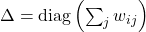 , the combinatorial Laplacian can be modeled as
(5) 
Each edge weight can be obtained as
(6) 
where  is the coordinate of voxel
  and
and  is its normalized structural intensity. The 2D phantoms use four neighbors. The notation
  indicates the corresponding six-neighbor construction for a 3D volume. In this way, nearby voxels with similar structural intensity receive strong coupling. A boundary reduces the weight and permits a sharper change in the estimated coefficients.
Convex Optimization Formulation
The global coefficient matrix  can be obtained as
(7) 
where  and
and  are regularization parameters and
(8) 
with  denoting the -th row of
  .
.
In the objective function in Equation (7), the first term enforces fidelity to the observed data by penalizing the mismatch between the measured signal  and its reconstruction
  . The second term can suppress an atom across the image rather than allowing it to appear only in a few noisy voxels. The last term measures the similarity between adjacent coefficient vectors via
  . In structurally homogeneous regions, the effect increases, while in areas near the edges where the corresponding weight is small, the effect weakens. By appropriately controlling the values of the weights of these three terms in Equation (7), the tradeoff among data fit, shared atom support, and spatial continuity can be adjusted.
Theorem 1 (Convexity of (7)). The objective function in (7) is convex in . Since the constraint set  is also convex, (7) constitutes a convex optimization problem.
Proof. Convexity is established term by term. (i) Data fidelity. The map  is a convex quadratic function of . (ii) Joint sparsity.
  is a norm and is therefore convex. (iii) Graph Laplacian smoothness. Since
  , there exists a matrix
  such that
  . Consequently,
 which is a sum of squared norms and therefore convex. (iv) Constraint set. The set is an intersection of half-spaces and is therefore convex. Combining these four properties establishes that (7) is convex.
Remark 1 (Global Minimums and Uniqueness). Convexity makes every local minimum of (7) a global minimum. Nonetheless, the uniqueness of the optimal solution is not guaranteed. To achieve uniqueness, every nonzero feasible direction  on the active support would need
  together with the relevant support conditions from the nonsmooth
  term. In this paper, a restricted minimum eigenvalue is not calculated and the active-support conditions for each experiment are also not verified. Thus, only the global optimality is claimed and not uniqueness.
Optimization Algorithm
The constrained primal problem (7) can be solved directly. The smooth part in the objective function can be given as
(9) 
so that
(10) 
The remaining component is  , where
  is the indicator of the non-negative orthant. For each row, the proximal update is
(11) ![\begin{equation*}\operatorname{prox}_{\eta(\lambda\lVert \cdot \rVert_{2,1}+I_{+})}(y) =\begin{cases}\left(1 - \dfrac{\eta\lambda}{\lVert y_+ \rVert_2}\right) y_+, & \lVert y_+ \rVert_2 > \eta\lambda,\\[1.5ex]0, & \lVert y_+ \rVert_2 \le \eta\lambda,\end{cases}\end{equation*}](https://nhsjs.com/wp-content/ql-cache/quicklatex.com-8d99baed0b3b01364447128e294cf55d_l3.png "Rendered by QuickLaTeX.com")
where  is evaluated element by element. The positive part enforces the constraint, while the row threshold applies joint sparsity. No later projection is required. The gradient Lipschitz constant satisfies
(12) 
so a conservative fixed step size is  . In practice, power iteration estimates
  and
and  , and a backtracking step is triggered if the objective does not decrease. The experiments use standard FISTA acceleration. It leaves the minimizer unchanged but required fewer iterations in the synthetic tests. Algorithm 1 demonstrates the entire procedure to solve the problem (7).
| Input | Data , dictionary  , graph Laplacian , parameters , , step size , graph Laplacian , parameters , , step size |
| Output | Coefficient matrix |
| 1 | Initialize  , ,  , and , and  |
| 2 | for  |
| 3 |  |
| 4 |  |
| 5 | for  |
| 6 |  |
| 7 | if  |
| 8 |  |
| 9 | else |
| 10 |  |
| 11 | endif |
| 12 | endfor |
| 13 |  |
| 14 |  |
| 15 | endfor |
| 16 | return  |
Computational complexity
Each iteration requires one multiplication by and one by  , with cost
  for dense dictionaries. The sparse graph multiplication
  costs
costs  . The row-wise proximal step costs
  . Thus the per-iteration cost is
  and memory storage is
  when the graph is stored sparsely. For 3D whole-brain applications, the dominant memory term is
  , so block-wise processing and sparse atom pruning are important implementation strategies.
Results
GR-MCQ was evaluated in two settings. A controlled synthetic phantom provides known coefficients for direct error measurement. A second, in-vivo-style anatomical phantom is examined with its construction labels withheld, so the analysis must rely on the kinds of proxy criteria available when ground truth is unknown.
Experimental Setup and Implementation Details
I used the optimization pipeline in the Optimization Algorithm section for every reconstruction. At each projected proximal-gradient iteration, Equation (11) imposes nonnegativity and joint sparsity. For reproducibility, Table 2 records the settings held in common across the experiments.
| Setting | Choice used in this study |
|---|---|
| Dictionary size | 120 atoms |
| Rician-test measurements | 96 |
| Diffusion weightings |  s/mm s/mm |
| Gradient directions | 6 uniformly spaced in-plane directions |
| Relaxation contrasts |  ms; ms;  ms ms |
| Orientation grid | 5 orientation groups |
| Diffusivity grid |  ; ;  mm/s mm/s |
| grid |  ms; ms;  ms ms |
| Regularization |  |
| Regularization |  |
| Graph connectivity | 4-neighbor (2D); 6-neighbor extension (3D) |
 (spatial) (spatial) | 1 voxel |
 (intensity) (intensity) | 0.15 after structural-intensity normalization |
| Optimization iterations | 300 |
| Step size |  |
| Stopping check | 300 iterations; objective recorded at each iteration |
| Initialization |  |
Dictionary and multi-contrast synthesis
For both experiments, the forward operator uses the extended relaxation-diffusion dictionary defined in (3). The original Gaussian-noise pilot uses one dictionary for both signal synthesis and reconstruction. The primary Rician comparison does the same. Two additional tests move the synthesis parameters off the reconstruction grid, allowing the dictionary to be tested as an approximation rather than an exact copy of the signal model.
Graph construction
The graph is built from the structural reference image using (6) and the connectivity in Table 2. An edge receives a large weight only when its voxels are close and have similar structural intensity. Thus two voxels inside a homogeneous region influence each other more than two voxels separated by a tissue boundary, even if both pairs are immediate grid neighbors.
Regularization parameters
Unless stated otherwise, the repeated simulations use  and
and  . Here controls row sparsity, or shared atom support across voxels, and mainly affects noise robustness. The parameter sets the strength of graph-guided coupling and mainly affects anatomical coherence.
Synthetic Phantom Validation
Experimental Setup
A 2D synthetic phantom was built with three kinds of regions: anisotropic white-matter-like tissue, isA 2D synthetic phantom was built with three kinds of regions: anisotropic white-matter-like tissue, isotropic tissue water, and free-water-like compartments. Multi-contrast measurements were synthesized according to the linear model
(13) 
where is the relaxation-diffusion dictionary,  is the ground-truth coefficient matrix, and
  is additive zero-mean Gaussian noise. Three reconstructions were compared: voxel-wise fitting, voxel-wise fitting followed by smoothing, and GR-MCQ.
Quantitative Evaluation
Coefficient recovery accuracy is measured using the relative Frobenius reconstruction error
(14) 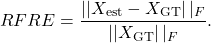
which was previously labeled NRMSE; the quantity is a normalized matrix error, computed over the full coefficient matrix, and is distinct from a root-mean-square voxel error. The structural similarity index (SSIM) is also computed between the reconstructed and ground-truth coefficient maps.
| Method | RFRE (%) | SSIM |
| Voxel-wise fitting | 15.2 | 0.92 |
| Voxel-wise + smoothing | 13.8 | 0.94 |
| Proposed (GR-MCQ) | 10.5 | 0.98 |
Table 3 shows GR-MCQ with the lowest RFRE and the highest SSIM among the compared methods in this pilot realization. The penalty suppresses noise-driven spurious atom activations, which stabilizes reconstruction, while the graph Laplacian enforces within-region consistency without sacrificing boundary sharpness where graph weights diminish. Because only a single realization is reported here, statistical significance is not claimed.
Qualitative Comparison
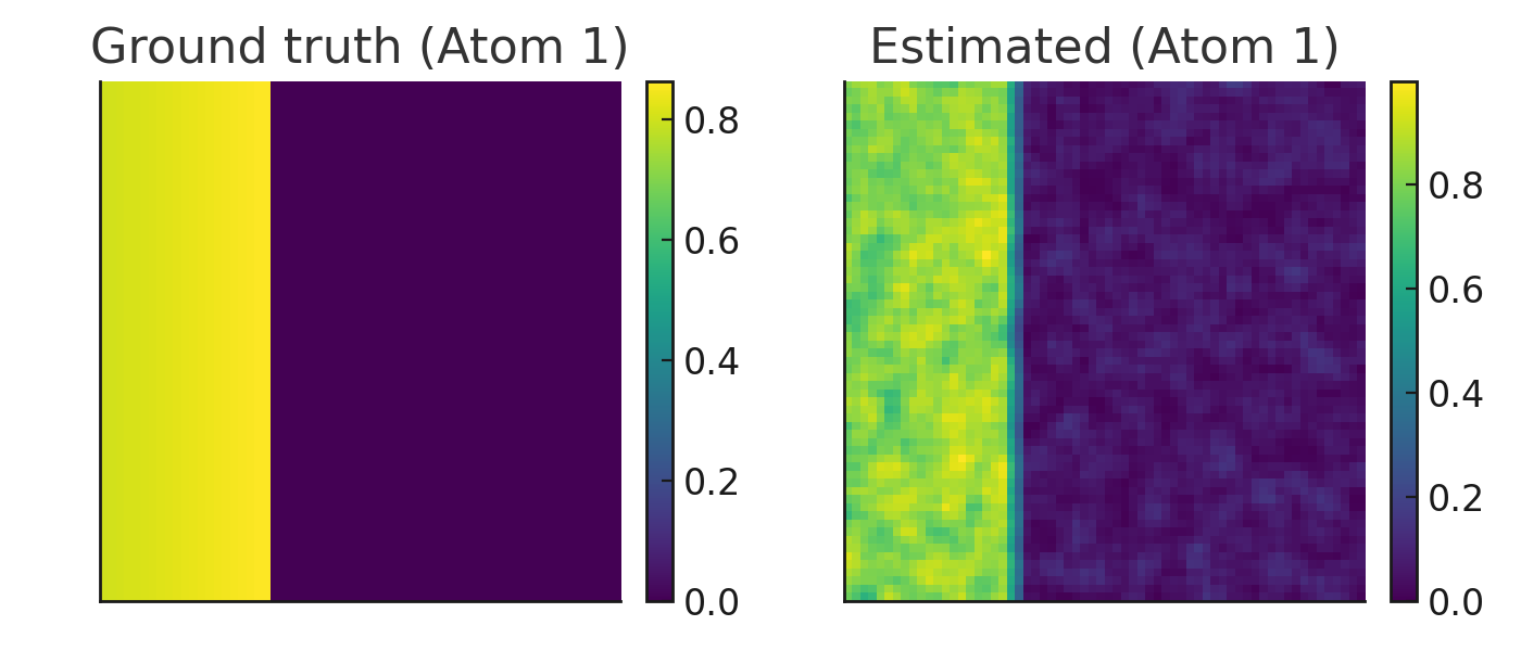
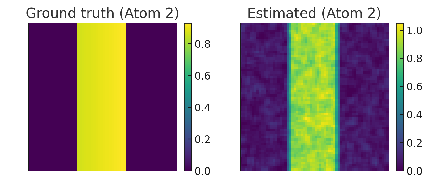
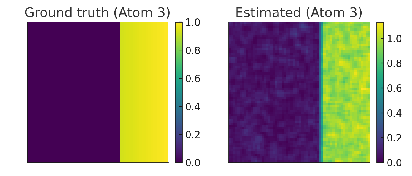
I inspected Figures 1-3 on the same coefficient scale. The boundary for Atom 2 looks slightly sharper than those for Atoms 1 and 3, but I did not test this visual difference for significance and therefore combine the atoms in the analysis below. The independently fitted voxel maps contain isolated errors. Smoothing removes part of that speckle, but the tissue transitions also become less distinct. In the GR-MCQ panels, many isolated fluctuations disappear while the region boundaries remain visible. That is the specific visual behavior the anatomy-weighted graph was designed to produce.
Rician-Noise Robustness and Repeated Simulations
Experimental Design
The Rician analysis used a  three-region phantom and the 120-atom dictionary. The acquisition followed the 96-measurement protocol in Table 2. For each SNR in
  , 30 independent magnitude-noise realizations were generated with fixed master seed:
(15) 
where  and
and  is the 95th percentile of the noise-free signal. Because atoms that differ only slightly in , , or diffusivity can be nearly indistinguishable, the primary Rician endpoint is computed after summing the 24 parameter variants within each of the five orientation-compartment groups:
(16) 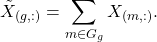
The group-level RFRE applies (14) to  . This endpoint tests recovery of the spatial compartment maps without claiming exact identification of every finely discretized atom.
Repeated-Noise Results
| Method | SNR 10 | SNR 20 | SNR 30 | SNR 40 |
|---|---|---|---|---|
| Voxel-wise fitting | 20.50 ± 1.36 | 9.84 ± 0.63 | 6.24 ± 0.40 | 4.23 ± 0.32 |
| Voxel-wise + smoothing | 37.21 ± 0.68 | 33.47 ± 0.24 | 32.50 ± 0.15 | 32.04 ± 0.09 |
| Proposed (GR-MCQ) | 17.24 ± 1.20 | 9.11 ± 0.54 | 6.17 ± 0.32 | 4.78 ± 0.28 |
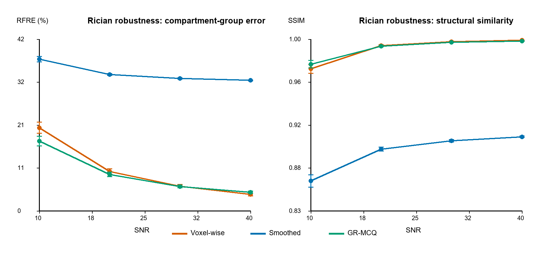
The most significant difference appears at SNR 10 which can be considered relatively noisy environment. Compared with voxel-wise fitting, the GR-MCQ reduces the paired RFRE by 3.27%, with a 95% confidence interval between 3.04 and 3.50. At SNR 20, the reduction is smaller, at 0.74% (0.61 to 0.86). At SNR 30, a difference of 0.06% is negligible, and that interval lies between -0.04 and 0.17. The tendency is reversed at SNR 40, where GR-MCQ has an error 0.56% higher. These results can be interpreted as a bias-variance trade-off. Coupling is useful when the noise is large, while regularization bias becomes significant with low noise-level. The post-smoothing results perform poorly at all SNR values since they average coefficients across the boundaries of the two sharp regions of the phantom.
Dictionary Mismatch
To reduce inverse-crime bias, additional SNR-20 experiments synthesize signals using shifted physical parameters while reconstruction retains the original grid. The mild mismatch scales both diffusivities by 1.025 and shifts by  ms; the moderate mismatch uses 1.05 and
  ms.
ms.
| Dictionary condition | Group RFRE (%) | SSIM |
|---|---|---|
| Matched | 9.21 ± 0.60 | 0.9930 ± 0.0008 |
| Mild mismatch | 10.08 ± 0.67 | 0.9916 ± 0.0010 |
| Moderate mismatch | 10.92 ± 0.71 | 0.9902 ± 0.0012 |
The moderate mismatch raises group RFRE by 1.71%. The increase is clear, although the reconstruction does not fail. Since this result comes from one controlled phantom sweep, it does not establish sensitivity across other tissue models, acquisition protocols, or dictionary resolutions.
Regularization Trade-off
The graph weight was swept over  at SNR 20 using 10 repeated noise realizations while holding
  fixed.
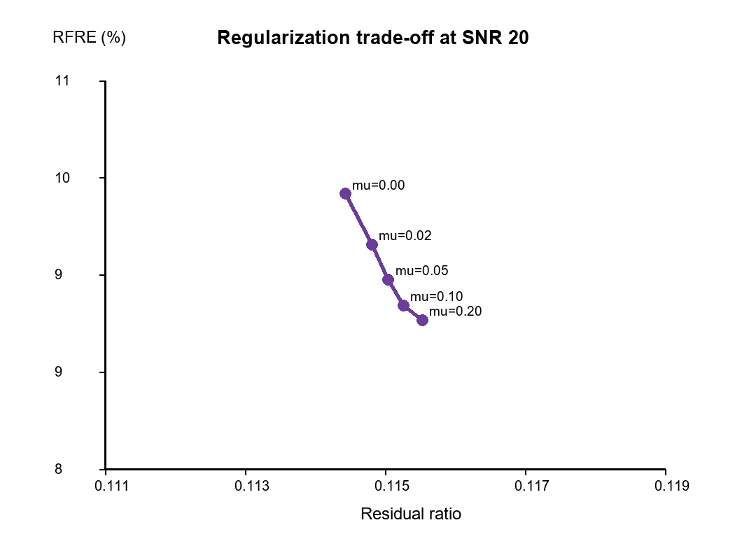
Increasing from 0 to 0.20 lowers mean group RFRE from 9.90% to 9.12%, while the residual ratio increases from 0.1142 to 0.1153. The curve gives a direct, quantitative view of the bias-variance trade-off, supplementing the qualitative explanation given above. The reported setting  sits near the bend of the curve, which avoids simply selecting the largest tested regularization value from this small phantom.
In-Vivo-Style Anatomical Validation
Experimental Design
A simple three-region geometry was replaced with a brain-like phantom with white matter (WM), gray matter (GM), and cerebrospinal fluid (CSF). Multi-contrast measurements are generated from tissue-specific diffusion and relaxation parameters. Bilateral graph weights are also derived from structural T1-weighted images. While analyzing, I deliberately hid the structure label. By visualizing them, residual ratio and coherence testing will become possible unlike patient scans without an actual microstructure map.
Representative Results
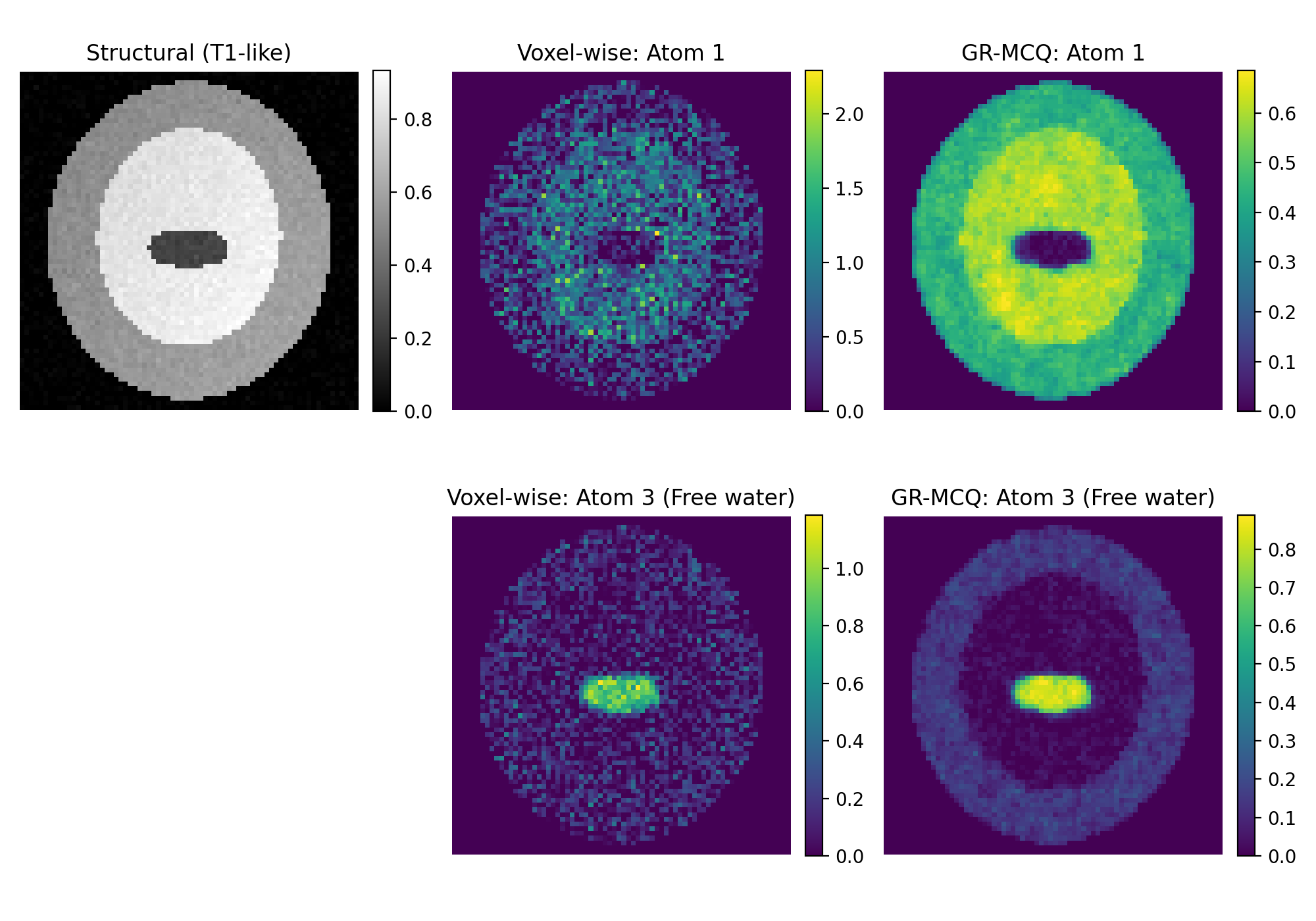
In Figure 6, the voxel-wise maps contain scattered coefficient changes with no corresponding feature in the structural reference. They are most noticeable around the WM-GM and GM-CSF interfaces. After graph regularization, most isolated values are gone and each tissue region is more continuous, yet the interfaces can still be seen. Equation (6) explains this result: a structural-intensity change lowers the edge weight, so coefficient vectors across the boundary pull less strongly on one another. For this phantom, the graph therefore improves within-region consistency without the broad edge blurring produced by an ordinary spatial filter.
Convergence Behavior
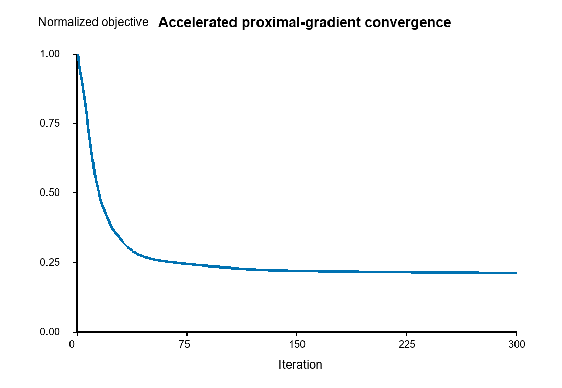
In Figure 7, the primal objective drops quickly at first and then levels off. With  iterations and the step-size rule in (12), the representative run reaches a stable plateau.
Proxy Quantitative Analysis Without Ground Truth
True in vivo microstructure parameters cannot be observed directly, so the anatomical-phantom analysis uses proxy criteria. One proxy is the relative residual fitting error,
(17) 
which measures data fidelity without requiring the unknown ground truth.
| Method | Residual Ratio |
| Voxel-wise fitting | 0.11 |
| Proposed (GR-MCQ) | 0.12 |
Table 6 shows similar data fidelity for GR-MCQ and voxel-wise fitting. The residual ratio rises modestly, from 0.11 to 0.12. In return, the Laplacian term produces a more spatially coherent estimate. Figure 5 measures this trade-off across the tested values of .
Reproducibility Analysis
For each of 30 paired trials, two independent SNR-20 Rician observations were generated and reconstructed separately. Consistency of the aggregated compartment maps is measured with ICC(3,1), a two-way mixed-effects, single-measure intraclass correlation suited to this repeated-measurement comparison28.
(18) 
where  is the between-target mean square,
  is the residual mean square, and
  is the number of repeated reconstructions. This is a simulation-noise reproducibility measure, not clinical scan-rescan reliability.
| Method | ICC(3,1) (mean ± std) |
| Voxel-wise fitting | 0.9945 ± 0.0006 |
| Proposed (GR-MCQ) | 0.9983 ± 0.0003 |
Both methods are highly consistent in this simple phantom (Table 7), and GR-MCQ adds a small increase. The joint sparsity prior discourages atoms from switching between reconstructions, while graph regularization shares stable support across anatomical neighborhoods. Both effects reduce sensitivity to the particular noise realization. These simulated pairs are not a substitute for clinical scan-rescan data.
Summary of Findings
I do not read these experiments as evidence of a uniform advantage. GR-MCQ has lower error in the Gaussian pilot and in the noisier Rician trials, but the difference nearly disappears at SNR 30 and changes direction at SNR 40. In the anatomical phantom, the visible boundaries remain, and the method stays stable in the particular dictionary-mismatch and repeated-noise tests performed here. The residual increase and convergence curve are also consistent with the expected cost of regularization. On that basis, I consider the algorithm feasible for further testing. I cannot draw a clinical conclusion because this study includes neither patients nor healthy volunteers.
Discussion
The main lesson I take from the phantom experiments is that contrast information and spatial information can be added to the same convex reconstruction without forcing every neighboring voxel to agree. In GR-MCQ, the relaxation-diffusion dictionary addresses compartment ambiguity, the term suppresses unstable atom choices, and the structural-MRI graph couples estimates only where the anatomy gives a reason to do so.
Since the formulated optimization problem in this paper is convex, it can be solved efficiently compared with other approaches such as voxel-wise non-linear fit. Specifically, GR-MCQ reduces coefficient errors at Gaussian pilot and low-to-mid-level Rician SNR, while improving map-to-map coherency without noticeable boundary loss. Furthermore, the residual ratio increases only slightly and the consistency of repeated noise improves.
I have kept the conclusions restricted to controlled synthetic and phantom data because no patient or healthy-volunteer scans were analyzed. A clinical study would need multi-contrast human data, protocol-variation and scan-rescan tests, appropriate preprocessing, and the required ethics and consent procedures. The SNR-40 result is especially important to this limit: GR-MCQ has slightly higher group RFRE than voxel-wise fitting, so regularization can do more harm than good when the measurements are already clean. I also observed a modest error increase under the moderate dictionary mismatch. That experiment covers only two off-grid shifts and should be expanded before drawing a general conclusion about mismatch.
Three-dimensional computation remains unresolved. With a dense dictionary, one iteration costs  and storing dominates memory. A whole-brain implementation will therefore need sparse dictionaries, block-wise reconstruction, GPU acceleration, or some combination of these. I did not make a matched wall-clock comparison with Levenberg-Marquardt fitting, AMICO, ADMM, or learned estimators. The complexity expression cannot substitute for timing all methods on
the same hardware with the same dictionary, voxel count, and stopping tolerance. Automatic selection of  would also be needed for practical use. For the next study, I would first improve the dictionary rather than add another regularizer. Better microstructural priors could address the original degeneracy while retaining the convexity and interpretability that motivated this approach.
References
- H. Zhang, T. Schneider, C. A. Wheeler-Kingshott, D. C. Alexander. NODDI: practical in vivo neurite orientation dispersion and density imaging of the human brain. NeuroImage. Vol. 61, pp. 1000-1016, 2012, https://doi.org/10.1016/j.neuroimage.2012.03.072. [↩]
- D. S. Novikov, E. Fieremans, S. N. Jespersen, V. G. Kiselev. Quantifying brain microstructure with diffusion MRI: theory and parameter estimation. NMR in Biomedicine. Vol. 32, e3998, 2019, https://doi.org/10.1002/nbm.3998. [↩]
- I. O. Jelescu, J. Veraart, E. Fieremans, D. S. Novikov. Degeneracy in model parameter estimation for multi-compartmental diffusion in neuronal tissue. NMR in Biomedicine. Vol. 29, pp. 33-47, 2016, https://doi.org/10.1002/nbm.3450. [↩]
- A. Daducci, E. J. Canales-Rodríguez, H. Zhang, T. B. Dyrby, D. C. Alexander, J.-P. Thiran. Accelerated microstructure imaging via convex optimization (AMICO) from diffusion MRI data. NeuroImage. Vol. 105, pp. 32-44, 2015, https://doi.org/10.1016/j.neuroimage.2014.10.026. [↩]
- G. Rensonnet, B. Scherrer, G. Girard, A. Jankovski, S. K. Warfield, B. Macq, J.-P. Thiran, M. Taquet. Towards microstructure fingerprinting: estimation of tissue properties from a dictionary of Monte Carlo diffusion MRI simulations. NeuroImage. Vol. 184, pp. 964-980, 2019, https://doi.org/10.1016/j.neuroimage.2018.09.076. [↩]
- E. Özarslan, C. G. Koay, T. M. Shepherd, M. E. Komlosh, M. O. İrfanoğlu, C. Pierpaoli, P. J. Basser. Mean apparent propagator (MAP) MRI: a novel diffusion imaging method for mapping tissue microstructure. NeuroImage. Vol. 78, pp. 16-32, 2013, https://doi.org/10.1016/j.neuroimage.2013.04.016. [↩]
- F. Pestilli, J. D. Yeatman, A. Rokem, K. N. Kay, B. A. Wandell. Evaluation and statistical inference for human connectomes. Nature Methods. Vol. 11, pp. 1058-1063, 2014, https://doi.org/10.1038/nmeth.3098. [↩]
- C. F. Caiafa, F. Pestilli. Multidimensional encoding of brain connectomes. Scientific Reports. Vol. 7, 11491, 2017, https://doi.org/10.1038/s41598-017-09250-w. [↩]
- Y. Wu, X. Liu, X. Zhang, K. M. Huynh, S. Ahmad, P.-T. Yap. Relaxation-diffusion spectrum imaging for probing tissue microarchitecture. In: Medical Image Computing and Computer Assisted Intervention-MICCAI 2023. Lecture Notes in Computer Science, Vol. 14227, pp. 152-162, 2023, https://doi.org/10.1007/978-3-031-43993-3_15. [↩]
- J. Hutter, P. J. Slator, D. Christiaens, R. P. A. G. Teixeira, T. Roberts, L. Jackson, A. N. Price, S. Malik, J. V. Hajnal. Integrated and efficient diffusion-relaxometry using ZEBRA. Scientific Reports. Vol. 8, 15138, 2018, https://doi.org/10.1038/s41598-018-33463-2. [↩]
- P. J. Slator, M. Palombo, K. L. Miller, C.-F. Westin, F. Laun, D. Kim, J. P. Haldar, D. Benjamini, G. Lemberskiy, J. P. de Almeida Martins, J. Hutter. Combined diffusion-relaxometry microstructure imaging: current status and future prospects. Magnetic Resonance in Medicine. Vol. 86, pp. 2987-3011, 2021, https://doi.org/10.1002/mrm.28963. [↩]
- S. Coelho, Y. Liao, F. Szczepankiewicz, J. Veraart, S. Chung, Y. W. Lui, D. S. Novikov, E. Fieremans. Assessment of precision and accuracy of brain white matter microstructure using combined diffusion MRI and relaxometry. Human Brain Mapping. Vol. 45, e26725, 2024, https://doi.org/10.1002/hbm.26725. [↩]
- S. Endt, M. Engel, E. Naldi, R. Assereto, M. Molendowska, L. Mueller, C. Mayrink Verdun, C. M. Pirkl, M. Palombo, D. K. Jones, M. I. Menzel. In vivo myelin water quantification using diffusion-relaxation correlation MRI: a comparison of 1D and 2D methods. Applied Magnetic Resonance. Vol. 54, pp. 1571-1588, 2023, https://doi.org/10.1007/s00723-023-01584-1. [↩]
- C.-F. Westin, H. Knutsson, O. Pasternak, F. Szczepankiewicz, E. Özarslan, D. van Westen, C. Mattisson, M. Bogren, L. J. O’Donnell, M. Kubicki, D. Topgaard, M. Nilsson. Q-space trajectory imaging for multidimensional diffusion MRI of the human brain. NeuroImage. Vol. 135, pp. 345-362, 2016, https://doi.org/10.1016/j.neuroimage.2016.02.039. [↩]
- I. S. Walimuni, K. M. Hasan. Atlas-based investigation of human brain tissue microstructural spatial heterogeneity and interplay between transverse relaxation time and radial diffusivity. NeuroImage. Vol. 57, pp. 1402-1410, 2011, https://doi.org/10.1016/j.neuroimage.2011.05.063. [↩] [↩]
- F. Zhang, E. R. Hancock. Riemannian graph diffusion for DT-MRI regularization. In: Medical Image Computing and Computer-Assisted Intervention – MICCAI 2006. Lecture Notes in Computer Science, Vol. 4191, pp. 234–242, 2006. https://doi.org/10.1007/11866763_29. [↩]
- L. M. Harrison, W. D. Penny, J. Ashburner, N. J. Trujillo-Barreto, K. J. Friston. Diffusion-based spatial priors for imaging. NeuroImage. Vol. 38, pp. 677-695, 2007, https://doi.org/10.1016/j.neuroimage.2007.07.032. [↩]
- G. Chen, Y. Hong, Y. Zhang, J. Kim, K. M. Huynh, J. Ma, W. Lin, D. Shen, P.-T. Yap. Estimating tissue microstructure with undersampled diffusion data via graph convolutional neural networks. In: Medical Image Computing and Computer Assisted Intervention–MICCAI 2020. Lecture Notes in Computer Science, pp. 280–290, 2020. https://doi.org/10.1007/978-3-030-59728-3_28 [↩] [↩]
- V. Golkov, A. Dosovitskiy, J. I. Sperl, M. I. Menzel, M. Czisch, P. Samann, T. Brox, D. Cremers. q-Space deep learning: twelve-fold shorter and model-free diffusion MRI scans. IEEE Transactions on Medical Imaging. Vol. 35, pp. 1344–1351, 2016. https://doi.org/10.1109/TMI.2016.2551324 [↩]
- C. Ye. Estimation of tissue microstructure using a deep network inspired by a sparse reconstruction framework. In: Information Processing in Medical Imaging. Lecture Notes in Computer Science, pp. 466–477, 2017. https://doi.org/10.1007/978-3-319-59050-9_37 [↩]
- R. Tanno, D. E. Worrall, A. Ghosh, E. Kaden, S. N. Sotiropoulos, A. Criminisi, D. C. Alexander. Bayesian image quality transfer with CNNs: exploring uncertainty in dMRI super-resolution. In: Medical Image Computing and Computer Assisted Intervention–MICCAI 2017. Lecture Notes in Computer Science, pp. 611–619, 2017. https://doi.org/10.1007/978-3-319-66182-7_70 [↩]
- T. Zheng, G. Yan, H. Li, W. Zheng, W. Shi, Y. Zhang, C. Ye, D. Wu. A microstructure estimation Transformer inspired by sparse representation for diffusion MRI. Medical Image Analysis. Vol. 86, 102788, 2023. https://doi.org/10.1016/j.media.2023.102788 [↩]
- Y. Li, Z. Zhuo, C. Liu, Y. Duan, Y. Shi, T. Wang, R. Li, Y. Wang, J. Jiang, J. Xu, D. Tian, X. Zhang, F. Shi, X. Zhang, A. Carass, F. Barkhof, J. L. Prince, C. Ye, Y. Liu. Deep learning enables accurate brain tissue microstructure analysis based on clinically feasible diffusion magnetic resonance imaging. NeuroImage. Vol. 300, 120858, 2024. https://doi.org/10.1016/j.neuroimage.2024.120858 [↩]
- D. Karimi, S. K. Warfield. Diffusion MRI with machine learning. Imaging Neuroscience. Vol. 2, 2024. https://doi.org/10.1162/imag_a_00353 [↩]
- H. Gudbjartsson, S. Patz. The Rician distribution of noisy MRI data. Magnetic Resonance in Medicine. Vol. 34, pp. 910-914, 1995, https://doi.org/10.1002/mrm.1910340618. [↩]
- C. G. Koay, P. J. Basser. Analytically exact correction scheme for signal extraction from noisy magnitude MR signals. Journal of Magnetic Resonance. Vol. 179, pp. 317-322, 2006, https://doi.org/10.1016/j.jmr.2006.01.016. [↩]
- J. Veraart, E. Fieremans, D. S. Novikov. Diffusion MRI noise mapping using random matrix theory. Magnetic Resonance in Medicine. Vol. 76, pp. 1582-1593, 2016, https://doi.org/10.1002/mrm.26059. [↩]
- T. K. Koo, M. Y. Li. A guideline of selecting and reporting intraclass correlation coefficients for reliability research. Journal of Chiropractic Medicine. Vol. 15, pp. 155-163, 2016, https://doi.org/10.1016/j.jcm.2016.02.012. [↩]