Abstract
This paper analyzes entanglement measures for tripartite systems of GHZ and W states. Von Neumann entropy quantifies the entanglement between subsystems. Concurrence quantifies pairwise entanglement in two-qubit reduced states. Monogamy characterizes how entanglement is distributed across the system. This expository analysis illustrates that, for the two ideal, symmetric three-qubit states considered here, no single measure fully captures the relevant entanglement structure, as each probes a distinct aspect of that structure. A more informative characterization of the two ideal, symmetric three-qubit states considered here requires using these measures together. Applied together, they reveal that the distinct behaviors of GHZ and W states reflect genuinely different entanglement architectures.
Keywords: Quantum Information, Multipartite Entanglement, GHZ State, W State, von Neumann Entropy, Concurrence, Monogamy
Introduction
Quantum entanglement1 is a fundamental property of composite quantum systems in which the state of the whole cannot be represented as a product of the states of its individual subsystems2,3. In this study, we focus on the GHZ and W states as representative examples of multipartite entanglement4 because they exhibit fundamentally different patterns of entanglement distribution among qubits. They belong to two inequivalent Stochastic Local Operations and Classical Communication (SLOCC) classes. It is a classification framework in which two entangled states are considered equivalent if one can be converted into the other via local operations and classical communication with nonzero probability of success5,6. To characterize these differences, this paper computes the von Neumann entropy, concurrence, and the squared-concurrence monogamy relation, and compares the results. No single measure can fully characterize multipartite entanglement, because each measure captures a different aspect of the entanglement structure. By analyzing these three measures together, this study avoids treating GHZ and W states as simply “more” or “less” entangled and instead highlights their distinct forms of entanglement. Together, these three measures support a multi-layered characterization of the entanglement structure. All calculations assume ideal, noiseless conditions; therefore, the conclusions drawn describe theoretical entanglement structure and may not directly apply to physical implementations where noise is present. This paper is an expository study that works through known results for GHZ and W states and asks how von Neumann entropy, concurrence, and three-tangle differ in what they capture and what they miss.
Methods
The GHZ state and W state are the two canonical representatives of genuinely tripartite entanglement. Genuinely tripartite entanglement implies that the entanglement involves all three qubits and is not described as only pairwise entanglement with one qubit left separable. Because both states are symmetric under any permutation of the qubits, all single-qubit entropies are equal, and all pairwise concurrences are equal. Therefore, it is sufficient to compute one representative single-qubit reduction and one representative two-qubit reduction. Despite the symmetry, the two states exemplify structurally distinct entanglement structures. The GHZ state represents global tripartite entanglement, in which the correlations are shared among all three qubits; removing any one qubit destroys the remaining pairwise entanglement, although classical correlations remain. The W state, in contrast, represents more locally distributed entanglement; after one qubit is removed, the remaining two qubits still retain pairwise entanglement. This structural opposition between fragility and robustness makes the states suited for comparing multipartite entanglement architectures.
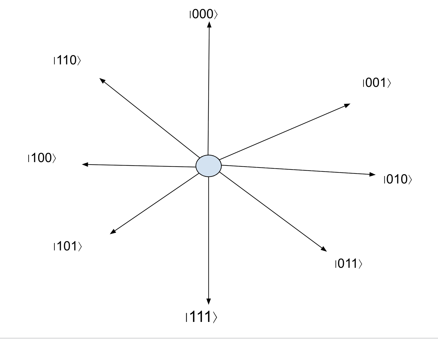
Both states are elements of an 8-dimensional Hilbert space7. This dimensionality follows from the tensor product structure of three qubits8. Each qubit has two basis states, |0⟩ or |1⟩ and the dimension of the Hilbert spaceis 23=8, corresponding to eight computational basis states. The diagram below illustrates the structure (Figure 1).
Within this framework of the Hilbert space, different three-qubit quantum states are distinguished by their amplitudes and correlations among the computational basis states. The GHZ and W states occupy specific, structurally distinct positions within this space. We apply three independent measures, von Neumann entropy, concurrence, and the squared-concurrence monogamy relation, to characterize both states quantitatively. These three measures were selected because they are standard analytic tools for three-qubit systems9,10 and because each captures a distinct structural feature: von Neumann entropy quantifies single-qubit mixedness, concurrence quantifies pairwise two-qubit entanglement, and three-tangle measures GHZ-type residual tripartite entanglement through the CKW monogamy relation.
Definition of GHZ and W states
The GHZ state11,12,13 is a superposition of two computational basis states, |000⟩ and |111⟩. Measuring one qubit in the computational basis collapses the superposition entirely into one branch, fixing the outcomes of the remaining qubits.
(1) 
(2) 
The W state14 is a superposition of three computational basis states, |001⟩, |010⟩, and |100⟩, with equal amplitudes. Measuring one qubit in the |0⟩ state eliminates only one branch, leaving the remaining two qubits in a superposition of the surviving components.
(3) 
(4) 
In this Hilbert space, the GHZ places equal amplitude on the two all-aligned basis states |000⟩ and |111⟩, whereas the W state places equal amplitude on the three-excitation basis, |001⟩, |010⟩, and |100⟩. The two states thus occupy inequivalent regions of the Hilbert space and cannot be transformed into one another, marking them as fundamentally distinct classes of tripartite entanglement.
Density matrix and partial trace
Both probability and coherence information are essential for understanding how qubits are entangled in the GHZ and W states. A density matrixrepresents the probabilities and quantum coherences of a quantum state. For a pure state |ψ⟩, the density matrix is obtained by taking the outer product 𝜌= |ψ⟩⟨ψ|. Because the GHZ and W states encode entanglement through both the likelihood of measuring each basis state and the correlations between qubits, the density matrix is the appropriate object for analyzing their structure.
(5) 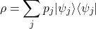
where pj is the probability weight associated with the state vector |ψj⟩, and ⟨ψj| is the corresponding bra vector. To analyze the information associated with individual qubits and their correlations with the rest of the system, we trace out the other qubits, obtaining a reduced density matrix for the selected qubits. This calculation is called a partial trace. The partial trace sums over an orthonormal basis of the subsystem being traced out, analogous to marginalization in classical probability. The partial trace is defined as follows:
(6) 
where A is an arbitrary linear operator on the Hilbert space.
Entanglement measures used in this study
To describe different layers of distribution, we applied von Neumann entropy, concurrence, and monogamy. The following subsections define these measures and explain their physical interpretations.
Von Neumann entropy
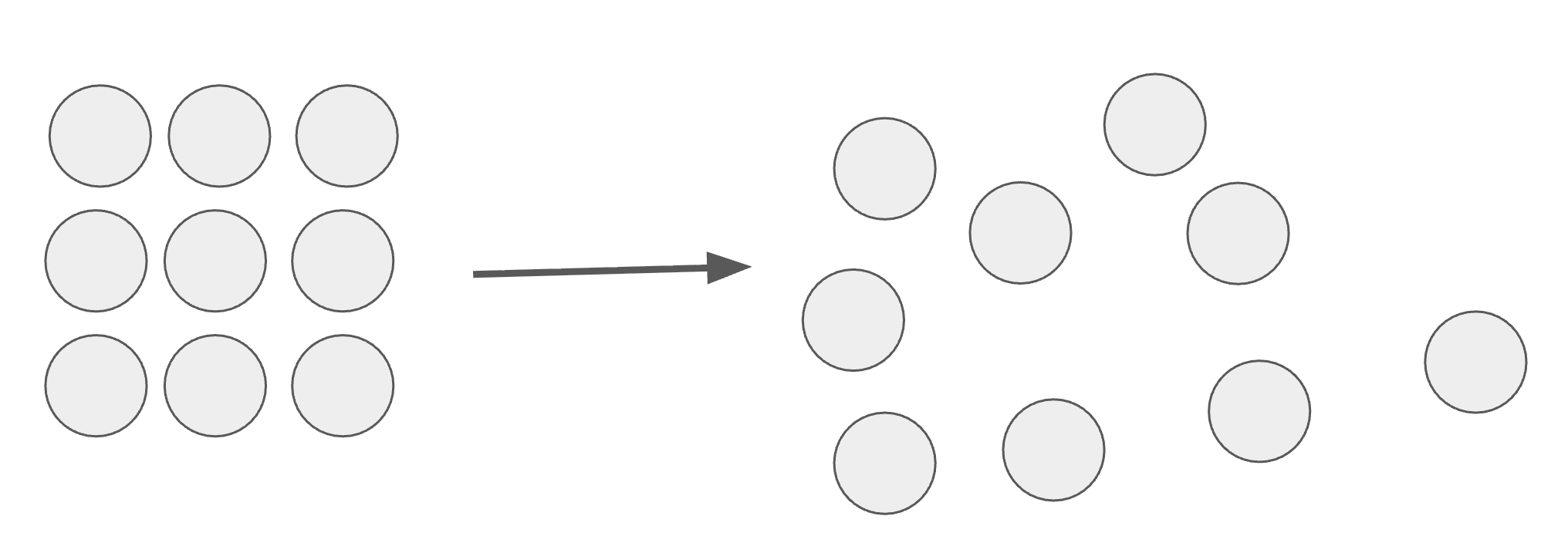
von Neumann entropyis a scalar measure of the mixedness of a quantum subsystem and serves as the standard entanglement quantifier for pure bipartite states15. The more entangled a subsystem is with other qubits in the system, the less its local state can be determined, signaling higher entropy. When a subsystem is maximally entangled with the other qubits in the system, its local state becomes completely undetermined, corresponding to maximum entropy. The diagram representing this is shown below (Figure 2).
The von Neumann entropy is then defined as16,17:
(7) 
The base-2 logarithm expresses entropy in units of bits. A von Neumann entropy value of 0 indicates that the subsystem is in a pure state. For a pure bipartite state, this means the subsystems are not entangled. For a single-qubit reduced state of a pure bipartite system, a von Neumann entropy value of 1 indicates maximal entanglement between the subsystem and its complement; equivalently, the reduced state is maximally mixed18.
Concurrence
Concurrence19 is a pairwise entanglement measure that quantifies the degree of entanglement between two qubits. Because it is strictly pairwise, it must be computed separately for each qubit pair. This requires isolating each of the three possible pairs in turn while discarding the third qubit. The diagram representing this is shown below (Figure 3).
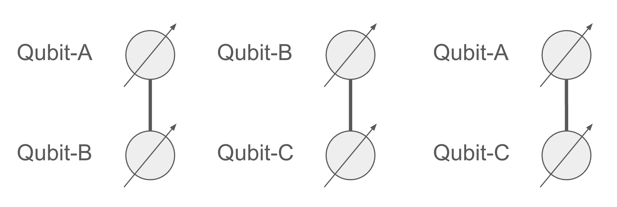
The spin-flipped density matrix  is defined by taking the complex conjugate of 𝜌 in the computational basis and applying 𝜎y to each qubit20
(8) 
(9) 
Here, 𝜌* denotes the elementwise complex conjugate of 𝜌 in the computational basis, and 𝜎y is the Pauli-Y operator.
A concurrence of 0 indicates the two-qubit state is separable — no pairwise quantum entanglement, though classical correlations may persist. A concurrence of 1 indicates maximal entanglement, characteristic of a Bell state.
(10) 
The eigenvalues of R are calculated, and 𝜆i are defined as the square roots of the eigenvalues of R, ordered from largest to smallest.
Monogamy
The monogamy relation, introduced by Coffman, Kundu, and Wootters(CKW), constrains how pairwise entanglement can be distributed across a multipartite system21,22. The CKW relation states that, for a pure three-qubit state, the squared entanglement between one qubit and the remaining pair is at least as large as the sum of its squared pairwise concurrences with each individual qubit. The diagram representing this is shown below (Figure 4).
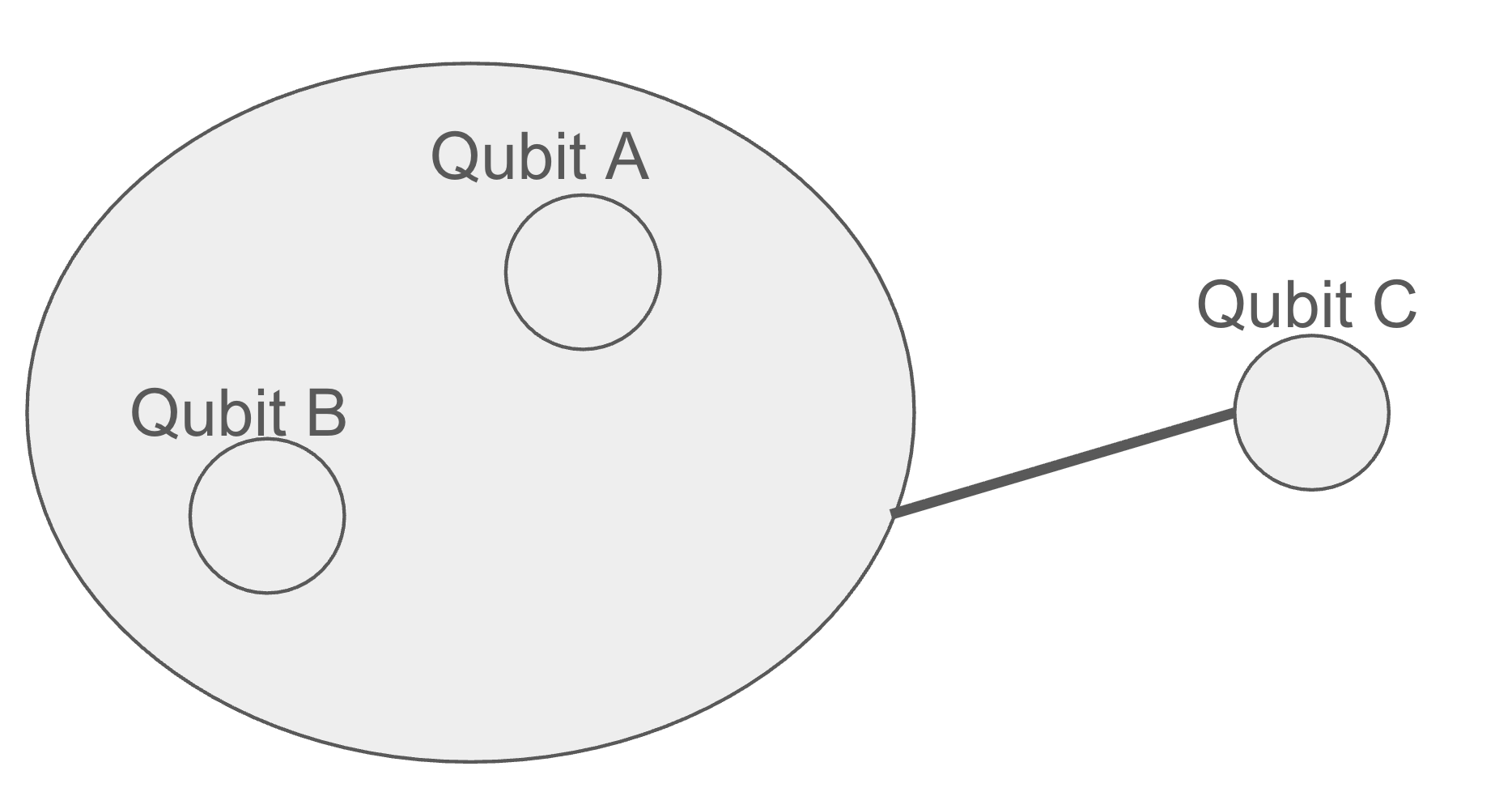
Monogamy is expressed as23:
(11) 
Here, a, b, and c label the first, second, and third qubits, respectively.
(12) 
(13) 
(14) 
Three-tangle is a scalar entanglement invariant that quantifies genuine tripartite entanglement in a pure three-qubit system and is defined as follows.
(15) 
For the symmetric GHZ and W states considered here, the residual tangle is independent of which qubit is chosen as the reference qubit. A three-tangle value of 0 indicates that this measure detects no GHZ-type residual tripartite entanglement; however, other forms of multipartite entanglement may still be present. The three-tangle value of 1 indicates maximal genuine three-qubit entanglement; physically, the entirety of the system’s information content is encoded nonlocally across all three qubits
Results
Von Neumann Entropy
To understand the differences in entanglement between the GHZ and W states, we apply the von Neumann entropy to evaluate the degree of entanglement between a subsystem and the rest of the system.
GHZ state
Converting the GHZ state vector into a density matrix operator requires calculating the partial trace. Then, the degrees of freedom belonging to qubit A are calculated by tracing out qubit B and C. The appendix contains the full calculations of the density matrix and partial trace of both cases: GHZ and W state.
(16) 
It is next written as a matrix to show explicit eigenvalues.
(17) 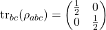
The eigenvalues of the matrix are ½ and ½. These identical values indicate equal probability for |0⟩ and |1⟩ on a subsystem A. Substituting into the von Neumann entropy formula yields:
(18) 
W state
Applying the same procedure used for the GHZ state, converting the W state vector into a density matrix operator requires calculating the partial trace.
(19) 
It is next written as a matrix to show explicit eigenvalues.
(20) 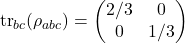
The eigenvalues of the matrix are ⅔ and ⅓. These unequal eigenvalues indicate that the reduced state of qubit A is not maximally mixed: outcome |0⟩ occurs with probability ⅔, while |1⟩ occurs with probability ⅓. Substituting into the von Neumann entropy formula yields:
(21) 
Concurrence
To quantify pairwise entanglement in the two-qubit reduced states of GHZ and W states, we applied concurrence.
GHZ state
Converting the GHZ state vector into a density matrix operator requires calculating the partial trace. Then, the degrees of freedom belonging to qubit B and C are calculated by tracing out qubit A. The appendix contains the full calculations of the density matrix and partial trace.
(22) 
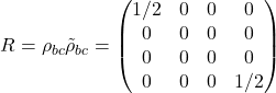
The ordered basis is taken to be |00⟩, |01⟩, |10⟩, |11⟩. The spin-flipped matrix ( ) follows from Eq. (8), which is explicitly expressed as:
(23) 
The matrix R from Eq. (9) is formed to explicitly expose its eigenvalues:
(24) 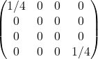
The eigenvalues are calculated from the matrix R, and the values are evaluated. The values of the eigenvalues R are 1/4, 1/4, 0, and 0. Therefore, the ordered square roots are 𝜆1=1/2, 𝜆2=1/2, 𝜆3=0, and 𝜆4=0.
Applying Eq. (10) gives
(25) 
W state
Converting the W state vector into a density matrix operator requires calculating the partial trace. Then, the degrees of freedom belonging to qubit B and C are calculated by tracing out qubit A. The appendix contains the full calculations of the density matrix and partial trace.
(26) 
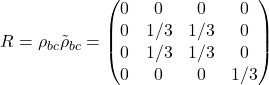
Using the ordered basis |00⟩, |01⟩, |10⟩, |11⟩, the spin-flipped matrix ( ) follows from its definition from Eq. (8), which is explicitly expressed as:
(27) 
The matrix R from Eq. (9) is formed to explicitly expose its eigenvalues:
(28) 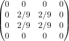
The eigenvalues are calculated from the matrix R, and the values are evaluated. The values of the eigenvalues R are 4/9, 0, 0, and 0. Therefore, the ordered square roots are λ1= 2/3, λ2= 0, λ3= 0, and λ4= 0.
Applying Eq. (10) gives
(29) 
Monogamy
To evaluate whether the GHZ and W states contain genuine tripartite entanglement that cannot be reduced to pairwise correlations, we apply the monogamy criterion.
GHZ state
The values of residual entanglement are calculated for the three-tangle, and two values are equivalent by GHZ state symmetry. The pairwise squared concurrences are equal to 0.
(30) 
The last residual entanglement component is calculated.
(31) 
Apply the definition of a three-tangle.
(32) 
W state
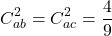
The residual entanglement, or three-tangle, is calculated using the monogamy relation. By symmetry of the W state, the pairwise squared concurrences are equal to 4/9.
(33) 
The last residual entanglement component is calculated.
(34) 
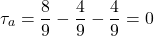
Apply the definition of a three-tangle.
(35) 
Discussion
Table 1 summarizes the values obtained from the three entanglement measures for the GHZ and W states.
| Von Neumann Entropy | Concurrence | Three-Tangle | |
| GHZ | 1 | 0 | 1 |
| W | 0.918 | 2/3 | 0 |
The GHZ state yields maximal von Neumann entropy, zero concurrence, and maximal residual tangle. The W state, by contrast, yields a 0.918 von Neumann entropy that confirms entanglement yet falls below the GHZ maximum, a concurrence of 2/3, and zero residual tangle. These values reveal the limitations of applying any single measure in isolation. Von Neumann entropy only measures the degree of mixedness of the reduced state; entropy alone cannot explain why GHZ loses pairwise entanglement upon qubit removal, although classical correlations remain. If interpreted alone, the zero pairwise concurrence of the GHZ reduced states could obscure the presence of genuine tripartite entanglement in the full state. This limitation is addressed by computing the three-tangle, which attributes the vanishing concurrence to entanglement distributed globally rather than pairwise. The three-tangle has a complementary limitation for the W state. Similarly, the three-tangle assigns zero to the W state, which could obscure the pairwise entanglement retained in its two-qubit reductions. This is because the three-tangle captures GHZ-type entanglement but does not register W-type entanglement. The three-tangle measures only the irreducible, collectively shared entanglement characteristic of GHZ states. In the W state, the entanglement detected after tracing out one qubit appears in the pairwise reduced states rather than in the GHZ-type residual tangle. The limitations of each measure are therefore complementary: each measure’s non-overlapping regions of insensitivity are covered by at least one of the remaining two. All calculations assume idealized, noise-free conditions; in practice, environmental noise may alter the outcome of each measure. Under local noise, GHZ-type coherence is generally fragile because it depends on the coherence between |000⟩ and |111⟩. Dephasing or depolarizing noise can rapidly reduce the three-tangle. W-type entanglement is often more robust to the loss of one qubit24 because tracing out one qubit can still leave an entangled two-qubit reduced state, although pairwise concurrence will also decrease under sufficiently strong noise. Other multipartite measures, such as negativity25,26, geometric entanglement27, and entanglement entropy across different bipartitions, could reveal additional aspects of the states; the present study focuses only on three standard analytic measures with clear interpretations for three-qubit systems. These calculations support the central argument that, for the ideal GHZ and W states considered here, the joint use of the three measures gives a more informative comparison of single-qubit mixedness, pairwise entanglement, and GHZ-type residual tripartite entanglement. A natural extension would be to study local depolarizing noise, in which each qubit is independently replaced by a maximally mixed component with some probability. One would expect GHZ-type three-tangle to be especially sensitive to the loss of global coherence, while W-state pairwise concurrence may be more robust under qubit-loss scenarios and may also persist under weak local noise, although a quantitative comparison would require explicit noise-channel calculations.
Conclusion
This expository study does not introduce a new entanglement measure or a new classification of GHZ and W states. Instead, it works through known results to show how von Neumann entropy, concurrence, and three-tangle provide complementary perspectives on the two ideal, symmetric three-qubit states considered here. Multipartite entanglement in GHZ and W states was characterized through three complementary measures: von Neumann entropy, concurrence, and three-tangle.
It is well established that no single measure can accurately characterize the entanglement structure of a multipartite system. Von Neumann entropy quantifies subsystem mixedness, concurrence isolates bipartite pairwise correlations, and the monogamy relation constrains the distribution of shared entanglement across subsystems. These measures were therefore applied jointly to resolve the entanglement structure of the states considered. The findings confirm that the distinct behaviors of GHZ and W states across these metrics reflect genuinely different entanglement architectures. GHZ states concentrate quantum correlations globally, so tracing out one qubit eliminates pairwise entanglement in the remaining reduced state, although classical correlations remain, whereas W states distribute entanglement across pairwise reduced states, preserving partial entanglement after one qubit is traced out. These distinctions become clear only when the states are examined through all three measures.
Appendix
A density matrix of the GHZ state is obtained by calculating |GHZ⟩⟨GHZ| by applying Eq. (5), where |GHZ⟩ and ⟨GHZ| are defined as Eqs. (1) and (2), respectively.
(A-1) 
The partial trace over qubits B and C is obtained by applying Eq. (6).
(A-2) 
Applying the same calculation procedure that was described in the previous section, the W state entropy is calculated. The main difference is the density matrix; the W state density matrix is obtained by computing |W⟩⟨W|, as defined in Eqs. (3) and (4), respectively.
(A-3) 
The partial trace over qubits B and C is obtained by applying Eq. (6).
(A-4) 
Concurrence
To evaluate pairwise entanglement in the two-qubit reduced states of GHZ and W, we take the partial trace over qubit A to obtain 𝜌BC and then apply concurrence.
(A-5) 
For the GHZ state, tracing out qubit A eliminates the off-diagonal terms because ⟨0|1⟩=0. The reduced density matrix 𝜌BC therefore contains only the diagonal terms |00⟩⟨00| and |11⟩⟨11|, which gives zero pairwise concurrence.
(A-6) 
For the W state, tracing out qubit A leaves both diagonal terms and off-diagonal coherence terms between |01⟩ and |10⟩. In particular, the terms |01⟩⟨10| and |10⟩⟨01| remain in 𝜌BC, which gives nonzero pairwise concurrence.
(A-7) 
References
- R. F. Werner. Quantum states with Einstein-Podolsky-Rosen correlations admitting a hidden-variable model. Phys. Rev. A. Vol. 40, pg. 4277-4281, 1989, DOI: 10.1103/PhysRevA.40.4277. [↩]
- A. Einstein, B. Podolsky, N. Rosen. Can quantum-mechanical description of physical reality be considered complete? Phys. Rev. Vol. 47, pg. 777-780, 1935, DOI: 10.1103/PhysRev.47.777. [↩]
- J. S. Bell. On the Einstein-Podolsky-Rosen paradox. Physics Physique Fizika. Vol. 1, pg. 195-200, 1964, DOI: 10.1103/PhysicsPhysiqueFizika.1.195. [↩]
- E. Schrödinger. Discussion of probability relations between separated systems. Proc. Cambridge Philos. Soc. Vol. 31, pg. 555-563, 1935, DOI: 10.1017/S0305004100013554. [↩]
- W. Dür, G. Vidal, J. I. Cirac. Three qubits can be entangled in two inequivalent ways. Phys. Rev. A. Vol. 62, pg. 062314, 2000, DOI: 10.1103/PhysRevA.62.062314. [↩]
- A. Acín, A. Andrianov, L. Costa, E. Jané, J. I. Latorre, R. Tarrach. Generalized Schmidt decomposition and classification of three-quantum-bit states. Phys. Rev. Lett. Vol. 85, pg. 1560-1563, 2000, DOI: 10.1103/PhysRevLett.85.1560. [↩]
- B. Schumacher. Quantum coding. Phys. Rev. A. Vol. 51, pg. 2738-2747, 1995, DOI: 10.1103/PhysRevA.51.2738. [↩]
- D. Deutsch. Quantum theory, the Church-Turing principle and the universal quantum computer. Proc. R. Soc. Lond. A. Vol. 400, pg. 97-117, 1985, DOI: 10.1098/rspa.1985.0070. [↩]
- O. Gühne, G. Tóth. Entanglement detection. Phys. Rep. Vol. 474, pg. 1-75, 2009, DOI: 10.1016/j.physrep.2009.02.004. [↩]
- R. Horodecki, P. Horodecki, M. Horodecki, K. Horodecki. Quantum entanglement. Rev. Mod. Phys. Vol. 81, pg. 865-942, 2009, DOI: 10.1103/RevModPhys.81.865. [↩]
- D. M. Greenberger, M. A. Horne, A. Zeilinger. Going beyond Bell’s theorem. In Bell’s theorem, quantum theory and conceptions of the universe; M. Kafatos, Ed. Kluwer, Dordrecht, 1989, pg. 69, arXiv: 0712.0921. [↩]
- D. M. Greenberger, M. A. Horne, A. Shimony, A. Zeilinger. Bell’s theorem without inequalities. Am. J. Phys. Vol. 58, pg. 1131-1143, 1990, DOI: 10.1119/1.16243. [↩]
- J.-W. Pan, D. Bouwmeester, M. Daniell, H. Weinfurter, A. Zeilinger. Experimental test of quantum nonlocality in three-photon Greenberger-Horne-Zeilinger entanglement. Nature. Vol. 403, pg. 515-519, 2000, DOI: 10.1038/35000514. [↩]
- M. Eibl, N. Kiesel, M. Bourennane, C. Kurtsiefer, H. Weinfurter. Experimental realization of a three-qubit entangled W state. Phys. Rev. Lett. Vol. 92, pg. 077901, 2004, DOI: 10.1103/PhysRevLett.92.077901. [↩]
- C. H. Bennett, D. P. DiVincenzo, J. A. Smolin, W. K. Wootters. Mixed-state entanglement and quantum error correction. Phys. Rev. A. Vol. 54, pg. 3824-3851, 1996, DOI: 10.1103/PhysRevA.54.3824. [↩]
- S. Popescu, D. Rohrlich. Thermodynamics and the measure of entanglement. Phys. Rev. A. Vol. 56, pg. R3319-R3321, 1997, DOI: 10.1103/PhysRevA.56.R3319. [↩]
- C. H. Bennett, H. J. Bernstein, S. Popescu, B. Schumacher. Concentrating partial entanglement by local operations. Phys. Rev. A. Vol. 53, pg. 2046-2052, 1996, DOI: 10.1103/PhysRevA.53.2046. [↩]
- V. Vedral, M. B. Plenio, M. A. Rippin, P. L. Knight. Quantifying entanglement. Phys. Rev. Lett. Vol. 78, pg. 2275-2279, 1997, DOI: 10.1103/PhysRevLett.78.2275. [↩]
- W. K. Wootters. Entanglement of formation of an arbitrary state of two qubits. Phys. Rev. Lett. Vol. 80, pg. 2245-2248, 1998, DOI: 10.1103/PhysRevLett.80.2245. [↩]
- S. Hill, W. K. Wootters. Entanglement of a pair of quantum bits. Phys. Rev. Lett. Vol. 78, pg. 5022-5025, 1997, DOI: 10.1103/PhysRevLett.78.5022. [↩]
- V. Coffman, J. Kundu, W. K. Wootters. Distributed entanglement. Phys. Rev. A. Vol. 61, pg. 052306, 2000, DOI: 10.1103/PhysRevA.61.052306. [↩]
- M. Koashi, A. Winter. Monogamy of quantum entanglement and other correlations. Phys. Rev. A. Vol. 69, pg. 022309, 2004, DOI: 10.1103/PhysRevA.69.022309. [↩]
- T. J. Osborne, F. Verstraete. General monogamy inequality for bipartite qubit entanglement. Phys. Rev. Lett. Vol. 96, pg. 220503, 2006, DOI: 10.1103/PhysRevLett.96.220503. [↩]
- A. R. R. Carvalho, F. Mintert, A. Buchleitner. Decoherence and multipartite entanglement. Phys. Rev. Lett. Vol. 93, pg. 230501, 2004, DOI: 10.1103/PhysRevLett.93.230501. [↩]
- G. Vidal, R. F. Werner. Computable measure of entanglement. Phys. Rev. A. Vol. 65, pg. 032314, 2002, DOI: 10.1103/PhysRevA.65.032314. [↩]
- A. Peres. Separability criterion for density matrices. Phys. Rev. Lett. Vol. 77, pg. 1413-1415, 1996, DOI: 10.1103/PhysRevLett.77.1413. [↩]
- T.-C. Wei, P. M. Goldbart. Geometric measure of entanglement and applications to bipartite and multipartite quantum states. Phys. Rev. A. Vol. 68, pg. 042307, 2003, DOI: 10.1103/PhysRevA.68.042307. [↩]