NHSJS Reports

Investigating the Significance of Socioeconomic and Built Environment Variables on Commuting Mode in the Delaware Valley Region

August 17, 2026

Abstract

How people commute, whether they drive or bike to work, shapes local environmental, health, and land-use outcomes, yet few studies have holistically examined commuting mode in the Delaware Valley Region—otherwise known as Greater Philadelphia. This study used multinomial logistic regression to determine which socioeconomic and built environment variables significantly influenced the commuting mode of individuals in the Delaware Valley Region. Socioeconomic variables included age, gender, race, income, vehicle ownership, and household size. Built environment variables included population density, land use diversity, transit density, destination accessibility, and street intersection density. The study finds that women were less likely to use active transportation than private transportation, while people of color were more likely to use both public and active transportation. Larger households and household vehicle ownership were associated with greater reliance on private transportation; notably, household vehicle ownership had the greatest association with commuting mode in the study. Among the built environment variables, higher population density and street intersection density were associated with greater use of public and active transportation, and higher destination accessibility was associated with greater active transportation. Unexpectedly, land-use diversity was positively associated with private transportation use. Overall, our study suggests that the built environment is not the sole determinant of commuting mode and may operate alongside—and at times be outweighed by—socioeconomic constraints such as vehicle ownership. Thus, these findings indicate that city planners should tailor their proposed policy interventions to the specific demographics of their city to obtain the most significant results.

Keywords: Built Environment, Commuting Mode, Delaware Valley Region, Greater Philadelphia, Multinomial Logistic Regression

Introduction

In recent decades, public opposition to car-centric infrastructure has increased dramatically due to various environmental, safety, and health concerns. For instance, in 2022, light-duty private vehicles alone contributed to 16% of total US emissions, producing 1000 million metric tons of CO2 equivalent¹. Motor vehicle accidents are also the leading cause of death for young people worldwide² and areas lacking proper pedestrian infrastructure are associated with higher obesity rates³. Thus, with the rise of movements such as New Urbanism, community leaders and urban planners alike have grown increasingly focused on introducing more sustainable methods of transportation to their communities.

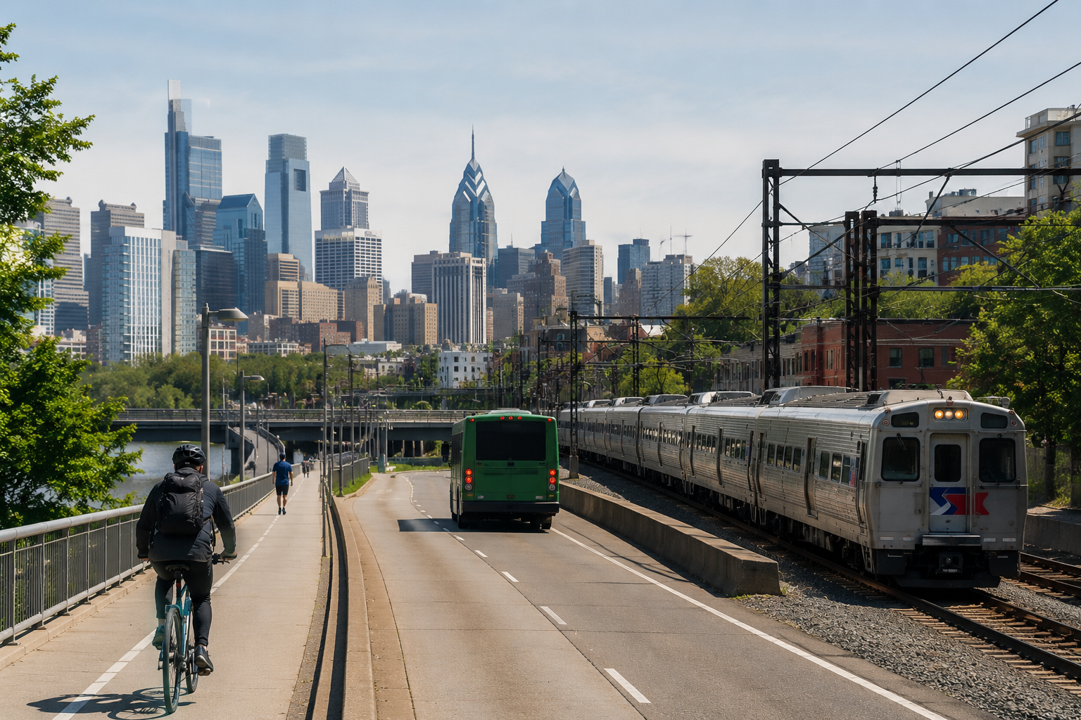
As a result, many studies have aimed to identify the underlying factors for an individual’s travel behavior and, more specifically, their chosen mode of transportation. However, significant gaps still remain. Firstly, many studies fail to compare the relative magnitudes of socioeconomic and built environment predictors of commuting mode, as prior literature has largely examined these two sets of factors separately. Moreover, few studies examine areas with both dense urban cores and dispersed suburban regions, and fewer still have examined the Delaware Valley Region—a region containing critical urban centers such as Philadelphia.

Thus, this study aims to analyze the impact of socioeconomic and built environment variables on commuting mode across the entirety of the Delaware Valley Region. Ultimately, this study finds that while the built environment significantly shapes commuting mode in the Delaware Valley Region, its influence is potentially outweighed by socioeconomic factors—particularly vehicle availability. Thus, our findings are consistent with a broader interpretation of commuting behavior which argues that commuting behavior is best understood not as a universal, predictable response to spatial incentives but as a complex behavior subject to varying habitual, social, and structural contexts.

Literature Review

Research on commuting mode can be separated into three overlapping strands. The first emphasizes the built environment, focusing on spatial incentives such as street intersection density and population density. The second emphasizes socioeconomic factors, arguing that individuals’ choices are constrained by factors such as age, vehicle availability, and race. The third examines behavioral and social variables, arguing that commuting mode is also impacted by factors such as habit, perceived risk, and social norms. The central tension between these explanations, therefore, is whether commuting behavior is primarily a response to spatial incentives or is instead constrained by socioeconomic and behavioral factors.

Literature concerning the relationship between the built environment and commuting behavior typically focuses on a combination of the following variables: density, diversity, design, distance to transit, and destination accessibility. These “5 D’s” were popularized by Ewing and Cervero (2010) and are commonly used as a framework in such studies⁴.

Density is commonly measured in terms of population, employment, and housing units. Studies have demonstrated that higher population, employment, and retail density have a negative association with car usage, instead encouraging active forms of transportation such as walking and biking as well as public transportation⁵^,⁶^,⁷^,⁸^,⁹^,¹⁰.

Diversity refers to a mix of different land uses as well as the jobs-housing balance in a region. Typically, more diverse and balanced land use mixtures tend to be negatively associated with the vehicle miles travelled (VMT) in a region by promoting alternative forms of transportation⁷^,⁹. This applies primarily to non-work trips since placing amenities like retail shops within residential areas, as opposed to outside them, reduces the need for automobiles¹¹; however, it also may apply to commuting trips by increasing the attractiveness of public transportation by situating local stores and markets near transit stops.

Design refers to a region’s street design, which includes features such as sidewalk lighting, sidewalk paving, block length, and intersection density. Street connectivity has been shown to have a positive relationship with both public transit use and active forms of transportation⁸^,¹⁰^,¹². Design measures such as 4-way intersections, sidewalks, and overhead streetlights have also all been found to promote public and active transportation⁷.

Distance from transit services has historically been a key focal point for literature related to transit-oriented development; it has been historically measured by transit route density, or an average of the distance between residences and employment centers from transit services. Greater proximity to transit stations has been shown to significantly encourage the use of transit⁶^,¹³^,¹⁴. Other studies have measured the correlation between the number of public transport vehicles and travel mode, finding that an increase in the number of public transit vehicles is associated with an increase in active transportation methods¹⁵.

Destination accessibility is frequently measured by distance from key services, such as grocery stores and parks, or, in the case of regional accessibility, determined by access to regional retail centers such as large shopping malls or central business districts. Literature concerning the impact of destination accessibility typically encompasses numerous different trip purposes, not only commutes, but their findings can still inform our understanding of how the built environment impacts commuting mode more generally. Handy (1993) found that both high levels of local and regional accessibility worked to decrease average shopping travel¹¹. Destination accessibility is also frequently determined through gravity-based models, such as the model used in Cervero and Kockelman’s study. Cervero and Kockelman (1997) found that public and active transportation use was greater in regions with greater destination accessibility⁷.

Built environment research typically emphasizes spatial opportunity and incentives. However, such studies typically share a common assumption: that commuters act as rational agents, constantly seeking to find the optimal commuting mode by evaluating constraints such as time, money, and convenience. A growing body of work, however, has instead argued that there exist socioeconomic factors as well as behavioral and habitual determinants that can similarly influence commuting mode, thus weakening the notion that commuting behavior is merely an optimization problem.

Innumerable studies have revealed the connections between socioeconomic variables, such as age or race, and mode choice. Using data from the 2001 National Household Travel Survey (NHTS), Pucher and Renne (2003) found that minorities and lower-income households account for roughly 63% of all transit users; however, even among the poorest, only 5% of their trips were made by transit, as the majority still predominantly relied upon private transportation¹⁶. In accordance with these findings from the NHTS, other regression-based studies have provided evidence that income may independently predict commuting mode, as it is shown to be positively associated with private transit use by numerous studies⁵^,¹⁵^,¹⁷. In their systematic review of 290 peer-reviewed mode choice behavior research papers, Ranjan and Sinha (2025) found that lower-income individuals relied on public transit more, as higher fuel costs and parking rates were key factors in determining whether an individual would primarily commute by car¹⁷. Falling travel costs, specifically the cost of driving a car in the US, have also been identified as a reason for this relationship. As the cost of commuting by car has fallen sharply in recent years to just 7% of daily wages, down from 20% of the daily income of a streetcar rider in the 1900s, higher-income households no longer value proximity to jobs as much as they previously did¹⁸. For those able to afford it, living in an area of their choosing is now much more appealing than living within close proximity to their job, as the cost of a longer commute, both financially and temporally, is relatively minimal.

Race and ethnicity have also been shown to play a role in travel behavior. When controlling for other variables, people of color are more likely than whites to walk and take public transit¹⁹. These patterns can be understood not solely as cultural preferences but also as the result of structural inequality. Decades of de jure and de facto segregation, as well as uneven transportation investment have concentrated people of color in areas with poor transit access and subpar infrastructure, drastically shaping the travel options available to them. Scholars such as Bullard (2003) have thus argued that the benefits of transportation systems in the United States have been distributed unequally along racial lines. From this perspective, instead of representing the independent effect of race, higher transit use among people of color reflects a legacy of segregated urban development that unfairly restricted vehicle access²⁰. However, it’s important to not overlook the nuance found within the relationship between race and commuting behavior. While other studies generally support Polzin et al.’s overall claim, they also highlight numerous other variations within different minority groups, such as the fact that Black individuals were less likely to use active transit than other minority groups²¹. In the United States specifically, commuting mode can vary among ethnic groups based on how recent their immigration was—recent immigrants are much more likely than native-born adults to use transit for commuting purposes²². Additionally, while all immigrants eventually undergo a process known as “transportation assimilation,” or essentially begin to adopt levels of automobile use more similar to their native-born counterparts, the rate of assimilation also varies by ethnicity. For instance, Asian immigrants are more likely than Hispanic immigrants to gravitate towards automobile use after 20 years of living in the US²².

Gender has also been found to be a significant indicator of commuting mode; in fact, a study released by the International Transport Forum that analyzed commuting behavior in cities across Europe and Asia suggests that gender may be a stronger determinant of mode choice than either income or age²³. Numerous studies have shown that women across different cities worldwide consistently prefer to take public transit more than men do⁶^,²³^,²⁴. Women have also been shown to be more likely than men to use certain forms of active transportation, such as walking²⁴. Importantly, however, this trend does not extend to cycling, as numerous studies have suggested that women are less likely to bike regularly to work than males²⁴^,²⁵. Both Goel et al. (2023) and Twaddle et al. (2010) suggest that this aversion to cycling may be due to safety-related issues²⁴^,²⁵. Goel et al. (2023) found that women who lived in cities with safe bike infrastructure like Berlin were more likely to bike than women in other cities, while Twaddle et al. (2010) found that when surveyed on potential barriers to cycling, women were more likely to cite safety concerns than men. A study done by Sims and Bopp (2018) on solely cities in the mid-Atlantic region of the US disagrees slightly with the findings presented by the aforementioned international studies done by Acker and Ng (2018) and Goel et al. (2023); they found that men are more likely to use both walking and biking for commuting purposes²¹^,²³^,²⁴. These divergent findings may have resulted from geographical scope and study design. Both the different demographical makeup of the primarily white American sample population of the study from Sims and Bopp (2018), as well as the comparatively poor pedestrian infrastructure found in the United States, may have deterred female survey respondents more than their counterparts in the studies of Goel et al. (2023) and Acker and Ng (2018)²¹^,²³^,²⁴.

Age has also been shown to play a role in commuting behavior. As individuals grow into old age, while they continue to rely on automobiles–as most older adults in the US still use a private vehicle weekly according to an analysis of the 2017 National Household Travel Survey–older adults (those above 50 years old) and younger adults (those below 30) are still more likely than middle-aged adults to use public transportation across nearly every continent¹⁷^,²⁶. In their systematic review, Ranjan and Sinha (2025) found that this greater transit usage was due to economic and physical reasons–for instance, younger individuals may not have earned the money needed to buy a car, while older individuals may prefer public transportation due to physical limitations¹⁷.

Perhaps intuitively, vehicle ownership or availability is consistently found to be one of the most significant predictors of commuting mode. Kitamura et al. (1997) found that vehicle ownership is positively associated with private transit use and negatively associated with both public transit and active transportation use¹⁴. Additionally, Susilo & Maat (2007) found that the impact of car ownership has significantly increased in past years, specifically by encouraging more private transit use and discouraging public transit use⁶.

Household size has similarly been shown to play a role in commuting mode. In their analysis on commuting behavior in the Delaware Valley Region, Guerra et al. (2018) found that household size was negatively associated with car-free travel²⁷. This pattern is consistently found in other studies as well, as larger households have been shown to be more likely to own automobiles⁸.

Taken together, this strand of research concerning socioeconomic factors suggests that mode choice is strongly constrained by variables such as income and age; under this perspective, commuting mode is not merely a reaction to the built environment but also a reflection of how race, gender, income, and household size can shape an individual’s access to transportation.

A separate body of work continues to question the theoretical validity of the rational-instrumental models implicitly assumed in most built environment studies by examining whether travel behavior is always the result of deliberate and logical mental processes. This body of work argues instead that commuting behavior is also impacted by behavioral and social processes, suggesting that choices regarding commuting mode can often be non-deliberate, and thus resistant to the cost-based incentives that form the foundation of rational-instrumental models.

For instance, car commuting can persist even when more convenient options are available, because changing from an inactive form of transportation to an active form involves breaking comfortable routines²⁸^,²⁹. Commuting decisions are frequently also influenced by risk aversion–when commuters focus primarily on the perceived risk and unreliability of a mode of transport rather than average travelling conditions³⁰. Subjective social norms can likewise play a significant role in shaping commuting behavior. After introducing a prepaid semester bus pass to German students, researchers found that the prepaid bus passes normalized bus ridership among the student body and thus contributed towards increased bus ridership³¹. These behavioral norms are not uniformly distributed across different genders, however; women show far stronger risk aversion than males, and thus commonly demonstrate a greater preference for safe cycling routes³².

Sociological work goes even further in dismantling the rational-instrumental model, arguing that commuting behavior is a routine social practice embedded within the intricacies of everyday life³³. Changing commuting mode can thus necessitate a complete overhaul of not only one’s morning commute, but also household arrangements and daily routines³³. Travel behavior is similarly impacted by social ties; Guell et al. (2012) observed that participants changed their commuting mode after an accident traumatized their spouse, or after a mother’s child-rearing responsibilities made her current commute impractical³³. In fact, certain active modes of transportation, such as biking, can even represent and form parts of an individual’s identity³³. From this perspective, the choice between private, public, and active transportation is not merely a cost-minimization exercise but instead is a deeply personal social practice tied to class, individual values, and environment³³.

Finally, it’s important to highlight a common methodological issue underlying these distinct stances regarding travel behavior: residential self-selection bias. Individuals who already prefer taking transit or using active modes of transportation may choose to live in dense, walkable, and transit-rich neighborhoods³⁴. Thus, associations between an individual’s commuting mode and their built environment may capture prior preferences, instead of indicating a causal impact of urban form³⁴. Methods typically utilized to reduce this bias have included controlling for relocation and repeating tests with differing levels of relocation among the study respondents³⁴.

Taken together, these studies indicate that commuting behavior is influenced by a complex, intricate web of disparate factors, ranging from spatial incentives to social norms. However, they each point towards two competing interpretations regarding commuting behavior. One holds that spatial incentives—such as street intersection density or transit accessibility—are the primary predictors of travel behavior. The other perspective holds that such effects are limited by socioeconomic or behavioral constraints. The Delaware Valley Region offers a fresh opportunity to compare these two perspectives and their relative strengths, as few prior studies have focused on the region.

Gap in Literature

While there have been many past studies that have focused on commuting behavior in American cities⁷^,¹⁴^,²¹, few such studies have focused on cities within the Delaware Valley Region. One notable study focusing on this region was done by Guerra et al. (2018)²⁷. However, while this study does examine the predictive impact of socioeconomic and built environment variables on travel behavior, it groups public transportation and active transportation into one “car-free” category while also omitting key built environment characteristics–namely destination accessibility and land-use diversity. Additionally, it’s rare for studies to examine both socioeconomic and built environment variables and compare their relative magnitudes. Choosing a heterogeneous area like the Delaware Valley Region is similarly uncommon; while studies such as that done by Acker and Ng (2018) may study commuting mode and its determinants in cities across multiple countries, few papers cover study areas with both predominantly suburban and urban areas²³. By testing variables across distinct urban forms, we can more easily eliminate the variables that are heavily context-specific and thus find the most robust predictors of commuting mode.

Thus, this study aims to address these gaps in the existing literature by examining the impact of socioeconomic and built environment variables on commuting mode in the Delaware Valley Region.

Methods

Study Area

The scope of the study was limited solely to the territories under the jurisdiction of the Delaware Valley Regional Planning Commission (DVRPC), the federally designated Metropolitan Planning Organization (MPO) for the Delaware Valley Region. The Delaware Valley Region is located in the northeast of the United States, encompassing 9 counties and 352 municipalities across Pennsylvania and New Jersey³⁵. The region is characterized by a blend of distinctly suburban and urban territories.

Following nationwide trends, the Delaware Valley Region has witnessed a massive decentralization of services and jobs, becoming more polycentric in nature. This reflects a broader transformation of American metropolitan regions. In the decades after WWII, jobs decentralized at roughly the same rate as residents, and thus their relative locations remained largely stable³⁶. As suburbs evolved from being simply bedroom communities to destinations that attracted major companies, workers and residents began to flood out of the inner city in favor of its surrounding suburbs. Consequently, the proportion of metro-area commutes that either began or ended in central cities fell sharply, from 66% in 1960 to 38% in 2000³⁶. As cities have continued to grow more polycentric, commuting patterns have grown in their complexity, becoming increasingly centered around suburban employment centers rather than one central location. The Delaware Valley Region has exemplified these broader trends, as future population estimates continue to predict rapid growth throughout its suburban counties³⁷. This massive suburban exodus may partially explain certain socioeconomic differences found across different areas in the Delaware Valley Region. For instance, Philadelphia’s median income is roughly $30,000 lower than that of Delaware County³⁸. Additionally, while Philadelphia is home to an extremely diverse population, Delaware County has a majority-white population³⁹.

Socioeconomic Characteristics

This subsection defines the socioeconomic variables used in the data analysis. For both socioeconomic and built environment variables, this study utilized data from the 2012-2013 Household Travel Survey (HTS) released by the Delaware Valley Regional Planning Commission (DVRPC) for both individual-level commuting behavior data as well as socioeconomic data. The survey included data on household and individual-level characteristics as well as individual trips by requiring all survey respondents to submit a one-day travel diary. Throughout the course of the study, 9235 total households were surveyed–although not all were used in the final data analysis.

For the purposes of this project, only individuals who had listed one of their destinations in their travel diary as a “work” destination were included. For the individuals who recorded two trips with destinations designated as “work,” only the trip with the longest recorded travel distance was considered. Other individuals were excluded from the analysis due to missing information. The final analysis included 5118 total individuals. Information on each individual’s age, gender, race, income, household vehicle ownership, and household size was taken from the HTS itself. In the original HTS, respondents were grouped into 10-year age cohorts. To ensure sufficient sample size in each age category, all ages below 34 and above 65 were grouped into their own categories, while the remaining age groups were preserved.Out of the 5118 individuals, 20.5% of individuals were between 1-34 years of age, 16.8% of individuals were between 35-44 years of age, 26% of individuals were between 45-54 years of age, 28.4% of individuals were between 55-64 years of age, and 8.4% of individuals were 65 years of age or older. A nearly identical number of respondents were male and female, with 2583 individuals being female and 2535 individuals being male. For the purposes of the study, all people of color were grouped into one category, while all white individuals constituted their own category, as the respondents were predominantly white. Since this aggregation overlooks meaningful heterogeneity among non-white individuals, the resulting coefficient is interpreted as a general contrast between ethnic minorities and white individuals, rather than a group-specific effect. Income was derived from the reported household income in the HTS. For the purposes of the study, all respondents with an annual household income of $0 to $49,999 were designated as “low income” (14%), all respondents with an annual household income of $50,000 to $149,999 were designated as “medium income” (63.3%), and all respondents with an annual household income of $150,000 and above were designated as “high income” (22.7%). These thresholds were informed by the Pew Research Center’s own income-tier framework⁴⁰. In our study sample, we found that 95.49% of individuals had a vehicle in their household. Furthermore, 13.52% of individuals lived alone, 38.20% of individuals lived in a two-person household, 20.57% of individuals lived in a three-person household, and 27.71% of individuals lived in a household with four or more individuals.

Variable	Categories	Count	Percentage
(a) Gender	Female	2583	50.47%
	Male	2535	49.53%
(b) Age group	1 to 34	1047	20.46%
	35 to 44	860	16.80%
	45 to 54	1332	26.03%
	55 to 64	1451	28.35%
	65 and above	428	8.36%
(c) Race	Other	515	10.06%
	White	4603	89.94%
(d) Household income	High income	1162	22.70%
	Low income	717	14.01%
	Medium income	3239	63.29%
(e) Household Vehicle Ownership	No Vehicle	231	4.51%
	Vehicle Available	4887	95.49%
(f) Household Size	One	692	13.52%
	Two	1955	38.20%
	Three	1053	20.57%
	Four or More	1418	27.71%

Table 1 | Sample characteristics from DVRPC 2012-2013 HTS (socioeconomic variables)

Built Environment Measures

This subsection describes the formulation of the built environment variables used in the final data analysis. A complete table listing the data sources and spatial scale for each of the built environment variables can be seen in Table 2.

This study considers built environment characteristics at the Traffic Analysis Zone (TAZ) level–the most granular level of geographic detail given in the DVRPC HTS–and municipal level. Street intersection density, population density, destination accessibility, and transit accessibility were all considered at the TAZ level, while land-use diversity was calculated at the municipal level. All built environment variables were matched to each individual based on their reported household TAZ.

Street intersection density was calculated as the number of residential street intersection nodes for each TAZ divided by the TAZ area, using the 2013 Census TIGER/Line Shapefiles.

Population density was determined by utilizing information from the 2010 US Census. Block-level population figures were aggregated to the TAZ level to determine population density for each TAZ.

In line with past studies concerning accessibility, destination accessibility was determined by using a gravity-based accessibility index at the individual level evaluated at each respective household TAZ⁷. This index is a property of the residential TAZ for each individual, capturing the degree to which an individual’s residential TAZ is connected to nearby employment opportunities. For each residential TAZ $i$ destination accessibility was computed as:

A_i = \sum_j O_j \cdot f(d_{ij})

Here, $O_j$ represents the number of jobs at a given destination TAZ $j$ while $f(d_{ij})$ is an impedance function which captures the travel cost between each origin TAZ $i$ and destination TAZ $j$ . Data for job figures on the TAZ level was taken from the 2013 US Census Bureau’s Longitudinal Employer-Household Dynamics Origin-Destination Employment Statistics (LODES) Workplace Area Characteristics. The sum of the product of both $O_j$ and $f(d_{ij})$ is then taken over all destination TAZs $j$ for each given origin TAZ $i$ to determine the final destination accessibility score $A_i$ .

The impedance function was determined using the following exponential decay function:

f(d_{ij}) = e^{-\beta d_{ij}}

$d_{ij}$ represents the shortest distance between the centroid of the origin TAZ $i$ and centroid of the destination TAZ $j$ through a road network determined by using the 2013 Census TIGER/Line Shapefiles.

The impedance coefficient $\beta$ was calibrated using the half-life criterion, which has been identified as a valid alternative to statistically estimated decay parameters⁴¹.

\beta = \frac{-\ln(0.5)}{m}

With this equation, a destination TAZ located at a distance exactly matching m, the regional median commuting distance, is given half the weight of an otherwise identical destination TAZ located at the origin TAZ. The regional median commuting distance was taken from the HTS itself.

In our analysis, we also considered internal travel distances, a core aspect of gravity-based accessibility measures⁴². For intrazonal terms where i=j, we approximated the internal distance of each zone, D_ij, as a function of its area:

D_{ij} = 0.5\sqrt{\frac{A_{zone}}{\pi}}

$A_{zone}$ represents the area of TAZ $i$ and was taken from the 2010 TAZ Boundaries Shapefile provided by the DVRPC. By using this formula, we represent each TAZ as a circle with equivalent area, and, following common practice, use one half of the circle radius to represent intrazonal travel distance⁴².

Transit accessibility was determined as the measure of the density of SEPTA and NJ Transit stops in each individual’s residential TAZ, using 2025 stop-level GIS files of all the metro, trolley, regional rail, and bus stops from SEPTA and NJ Transit’s systems. Though historical stop-level data for SEPTA’s transit system was available for the 2010s, no publicly available 2012-2013 NJ Transit stop-level data was able to be found. Prioritizing internal consistency, we thus used the 2025 transit stop datasets from both transit agencies as a rough approximation of transit accessibility for this study.

Land-use diversity was determined by using the Shannon-Wiener Diversity Index and was calculated at the municipality level. Land-use information was taken from the 2015 DVRPC land-use file.

H = -\sum_{i=1}^{S} p_i \ln(p_i)

$p_i$ represents the proportion of the entire municipality made up of land-use type $i$ . This figure was then multiplied by the natural log of itself and replicated for each land-use type. The sum of the calculated figures of each land-use type was then found and negated to determine the final index score for the municipality, H. This particular diversity index was chosen in order to account for both richness and evenness of land uses in a particular municipality. The index score for each municipality was then assigned to all the TAZs that fell under its jurisdiction, which was then matched to the reported household TAZ of each individual.

Variable	Data source	Spatial scale
Street Intersection Density	2013 Census TIGER/Line Shapefiles	TAZ
Population Density	2010 U.S. Census	TAZ
Destination Accessibility	2013 LODES Data, 2013 Census TIGER/Line Shapefiles	TAZ
Transit Density	2025 SEPTA and NJ Transit GIS files	TAZ
Land-Use Diversity	2015 DVRPC land-use file	Municipality

Table 2 | Built Environment Variables: Data Sources and Spatial Scale

Variable	Count	Mean	St. Dev	Max	Min
Street Intersection Density	5118	51.55032884	57.52800618	502.609	0.325
Population Density	5118	2870.044816	4389.319074	50279.38649	0
Transit Density	5118	14.15367176	35.63306214	581.2609876	0
Land-Use Diversity	5118	1.732121542	0.269508685	2.158370769	0.52974688
Destination Accessibility	5118	13913.30844	28818.82335	183985.1706	27.8579652

Table 3 | Descriptive Statistics for Built Environment Variables

Commuting Behavior Characteristics

Information on each trip’s given mode of transportation to work was likewise taken from the HTS. Different modes of transportation were grouped into three categories: Active Transportation, Public Transit, and Private Transportation. Active Transportation included modes such as walking and biking. Public Transit encompassed riders who utilized any form of SEPTA and NJ Transit service. Private Transportation included modes such as driving a car, carpooling, or using services from private transportation companies such as Greyhound.

Private transit was by far the most used mode of transportation, accounting for 84% of all respondents, whereas 8.3% of respondents used active transport and 8% of respondents used public transit.

Regression Modelling

The study utilized multinomial logistic regression to model the relationship between both socioeconomic and built environment variables and commuting mode, as shown below. The dependent variable in this study was the mode of commuting (private transit, public transit, and active transit). The independent variables included the socioeconomic and built environment variables. This particular model was chosen for its ability to handle a categorical dependent variable with more than two distinct categories, demonstrated by its common usage in previous studies⁶^,¹⁰^,²³.

\ln\left(\frac{P(Y=j)}{P(Y=k)}\right) = \beta_{0j} + \beta_{1j}X_1 + \beta_{2j}X_2 + \cdots + \beta_{pj}X_p

$\ln\left(\frac{P(Y=j)}{P(Y=k)}\right)$ represents the natural log of the ratio of the probability of choosing category $j$ over category $k$ (the reference category), also referred to as the log-odds. In this study, this represents the likelihood that one mode of transportation is chosen over another. Each coefficient $\beta$ represents the expected change in the log-odds of choosing category $j$ over the reference category for its designated variable $X$ . A positive coefficient represents a higher likelihood of choosing category $j$ over category $k$ , while a negative coefficient represents a lower likelihood of choosing category $j$ over category $k$ (and as such represents a higher likelihood of choosing category $k$ ).

By using this model, we can determine the association between each of our independent variables and each commuting mode. For our model, private transportation was chosen as our reference category as it is the most common mode of transportation among survey respondents. Furthermore, it reflects one of our study’s aims to identify the relationship between socioeconomic and built environment variables with car dependency. After the model was run, a Variance Inflation Factor (VIF) test was run to test for multicollinearity.

Results

Active Transportation	Coef.	P > \|t\|	Odds Ratio*	Public Transportation	Coef.	P > \|t\|	Odds Ratio*
const	0.904631	0.080453	2.47102	const	0.287898	0.576386	1.333622
Female	-0.28281	0.015369	0.753666	Female	-0.07768	0.493516	0.925265
Aged 1–34	-0.07229	0.675628	0.93026	Aged 1–34	0.155519	0.354626	1.168264
Aged 35–44	-0.01568	0.931739	0.984443	Aged 35–44	0.058934	0.745299	1.060706
Aged 55–64	-0.15033	0.365342	0.860424	Aged 55–64	-0.07248	0.661006	0.930083
Aged 65 and above	-0.31802	0.192328	0.727585	Aged 65 and above	0.034007	0.881757	1.034592
Non-White	0.376928	0.026086	1.457799	Non-White	0.762475	5.18E-07	2.143576
Low Income	0.094136	0.579133	1.09871	Low Income	-0.11006	0.51126	0.89578
High Income	0.280592	0.053615	1.323913	High Income	0.220224	0.129055	1.246356
One Person Household	0.071483	0.680395	1.0741	One Person Household	-0.13259	0.44351	0.875828
Three Person Household	-0.02173	0.892448	0.978506	Three Person Household	-0.22711	0.155077	0.796837
Four or More Person Household	-0.39396	0.01902	0.674384	Four or More Person Household	-0.41576	0.009167	0.659838
Vehicle Ownership	-3.07286	5.99E-31	0.046289	Vehicle Available	-3.13758	1.11E-32	0.043388
Population Density	8.5E-05	0.00014	1.452076629	Population Density	0.000116	3.9E-07	1.66359682
Transit Density	-2E-05	0.991672	0.999275127	Transit Density	-0.00059	0.776184	0.979045765
Land-Use Diversity	-0.54926	0.024608	0.862404969	Land-Use Diversity	-0.14354	0.551893	0.962054071
Street Intersection Density	0.003534	0.021706	1.225475727	Street Intersection Density	0.003163	0.046892	1.199595018
Destination Accessibility	1.15E-05	6.37E-05	1.39443151	Destination Accessibility	1.24E-06	0.685161	1.036479672

Model Fit Statistic	Value	Model Fit Statistic	Value
McFadden’s Pseudo R-squared	0.193	Likelihood-Ratio χ²	1100.6
Akaike Information Criterion (AIC)	4668.4122	Df Model	34
Log-Likelihood	-2298.2	Likelihood-Ratio χ² p-value	3.49E-209
LL-Null	-2848.5

Table 4 | Multinomial logistic regression for commuting behavior
*Odds ratios for continuous built-environment variables reflect a one-standard-deviation increase (SD’s shown in Table 3)

Variable	VIF
const	86.818218
Population Density	4.454203
Destination Accessibility	4.159453
Street Intersection Density	3.734973
Transit Density	2.353882
Aged 55-64	1.609676
Four or More Person Household	1.518147
Aged 1-34	1.495952
Aged 35-44	1.412416
Vehicle Ownership	1.310140
Three Person Household	1.306392
One Person Household	1.300113
Aged 65 and above	1.299491
Land Use Diversity	1.220565
Low Income	1.218412
High Income	1.097690
Non-White	1.066259
Female	1.017423

Table 5 | Results of VIF Test

A multinomial logistic regression model was used to determine the association between socioeconomic and built environment variables with commuting mode. The statistical analysis included 5118 individuals from the 2012-2013 DVRPC Household Travel Survey. Results from the VIF test were all below the conventional threshold of 5, indicating that multicollinearity was not a concern and that variable coefficients are reliable (Table 5).

Using private transportation as the reference category, we see that several variables were significantly associated with the likelihood of choosing public transportation compared to private transportation and choosing active transportation compared to private transportation (Table 4).

When comparing active transportation (e.g., walking or cycling) to our reference category (private transit), we find clear trends. Women were less likely to use active forms of transportation (coef = −0.2828, p = 0.015) compared to private transportation. People of color were more likely to use active forms of transportation (coef = 0.3769, p = 0.026). Individuals living in households with four or more people were also more likely to rely on private transportation (coef = −0.3940, p = 0.019). Individuals in a household with a vehicle were similarly associated with greater private transportation use (coef = −3.0729, p < 0.001). Higher population density encouraged more active modes of transportation (coef = 0.0000850, p < 0.001). Higher land-use diversity was associated with decreased active transportation (coef = −0.5493, p = 0.025). Higher street intersection density was also correlated with more active transportation use (coef = 0.0035, p = 0.022). Finally, destination accessibility was positively associated with active transportation use (coef = 0.0000115, p < 0.001).

Clear correlations also emerged when comparing public transportation to private transportation. Here, a positive coefficient for a given variable can be interpreted as an association with a greater use of public transportation. People of color were more likely to use public transit (coef = 0.7625, p < 0.001) compared to private transportation. Individuals living in households with four or more people were more likely to rely on private transportation (coef = −0.4158, p = 0.009). Individuals in a household with a vehicle were also more likely to use private transportation (coef = −3.1376, p < 0.001). Higher population density was positively associated with public transit use (coef = 0.000116, p < 0.001). Higher street intersection density also encouraged more public transit use (coef = 0.0032, p = 0.047). All other variables were not deemed statistically significant.

To compare the effect magnitudes of the categorical variables and continuous variables, coefficients were converted into odds ratios (OR). Odds ratios above 1 indicate a greater likelihood of choosing either active or public transportation over private transportation, while odds ratios lower than 1 indicate a lower likelihood. For the continuous built-environment variables, whose per-unit coefficients are very small and not directly comparable to categorical variables, ORs were instead scaled to a one-standard-deviation increase (SDs can be found in Table 3).

Vehicle availability was by far the strongest predictor across all modes, reducing the odds of choosing active or public transportation over private more so than any other variable (OR ≈ 0.05 and OR ≈ 0.04). Race was the next most influential factor, though exerting a larger impact in regard to transit (OR ≈ 2.1) than for active transportation (OR ≈ 1.5). Household size behaved similarly across both modes, as individuals in four-or-more-person households were significantly less likely to use either active or public transportation relative to private (OR ≈ 0.67 and 0.66). Gender was significant only for active transportation use (OR ≈ 0.75). Among the built-environment variables, higher population density and street intersection density were each consistently associated with greater use of both non-private modes (OR ≈ 1.45 and OR ≈ 1.23 for active transportation; 1.66 and 1.20 for public transportation). Higher destination accessibility was associated with greater active transportation use (OR ≈ 1.39) but was not a significant predictor of public transit. Contrary to expectations, higher land-use diversity was associated with lower active transportation use (OR ≈ 0.86). Overall, these results suggest that both socioeconomic and built environment factors are associated with commuting mode, but household vehicle ownership showed the greatest influence on commuting mode by far.

Discussion

Consistent with our central argument, individual socioeconomic factors, particularly vehicle ownership, influenced commuting behavior more consistently and powerfully than any built environment characteristic.

When comparing active transportation to private transportation, we find that gender, race, household size, vehicle ownership, population density, land-use diversity, street intersection density, and destination accessibility have a statistically significant impact. Our results when comparing the likelihoods of using public or private transit demonstrate that race, household size, vehicle ownership, population density, and street intersection density are the most significant determinants of mode choice. Our finding that women are less likely to use active transportation disagrees with findings from Goel et al. (2023) yet agrees with those of Sims & Bopp (2018)²¹^,²⁴. These disparities may be in part due to differences in study area; like Sims & Bopp (2018), our study was completed solely in the US, as opposed to the international nature of the study completed by Goel et al. (2023), which included 13 separate countries. This difference in study area may have been significant, as the United States is notorious for providing poor pedestrian and bicyclist facilities when compared to other developed nations⁴³. Indeed, pedestrian fatality rates in the US are still notably higher than other developed countries such as the UK, Germany, and the Netherlands⁴³. Thus, the drastic difference in quality of active transportation facilities between the study areas of these studies may have contributed to their differing results, especially considering that women–at least in this context of active transportation–have been previously shown to be more risk-averse than men. Indeed, in their study, Goel et al. (2023) found that women were especially less likely to bike than men in cities with poor cycling infrastructure, and Twaddle et al. (2010) found that women cited safety as a barrier to cycling more often than men did²⁴^,²⁵. These findings demonstrate that women, more than men, may require adequate pedestrian and cycling facilities in order to cycle regularly.

Race also emerges as a significant determinant of commuting mode, as people of color are more likely to rely on active transportation when compared to white individuals, a result supported by past studies¹⁹^,²¹. However, it’s important to note that such a result may mask significant variety even among different ethnic groups. Sims & Bopp (2018) found that though most people of color tended to use active transportation more than white individuals, African Americans demonstrated the least active transportation usage overall²¹.We also find that non-white individuals, with all else held constant, are associated with higher rates of public transportation. This agrees with findings from past literature, possibly explained by a greater awareness of transit services among minority groups, as well as decreased stigma associated with using public transportation¹⁹^,²¹. This finding can also be understood through the lens of structural inequality. Elevated transit use among people of color may reflect historical disparities in income or residential location stemming from decades of segregation and discrimination¹⁹^,²⁰.

Our finding that individuals in households with four or more people were more likely to use private transportation when compared to both active and public transit is consistent with prior research²⁷. As a result, this finding may indicate that larger households face more complex travel patterns than smaller households, thus gravitating towards the flexibility offered by a private vehicle.

Vehicle ownership emerged as the strongest predictor of commuting mode in our study, as individuals in a household with a vehicle were far more likely to use private transportation over active transportation and public transportation. This is strongly consistent with past literature¹⁴^,⁶.The dominance of this variable in studies conducted across distinct nations and landscapes suggests that vehicle availability may overshadow built environment characteristics when determining individual commuting mode. The findings from our study and others indicate that even within built environments generally associated with transit-supportive characteristics, household vehicle ownership still remains a dominant predictor of commuting mode.

The dominance of vehicle ownership in our model may also indicate the role of habit in commuting. Car users typically show significant resistance to switching modes as car use evolves into a habit, making drivers resistant to different modes of transportation²⁸. Thus, this deterrence towards changing car-usage habits among drivers may partially explain why vehicle ownership so strongly predicted private vehicle use.

However, our model still demonstrates that certain measures of urban form influence commuting mode. For instance, street intersection density was shown to significantly increase the likelihood of active transportation use, similarly falling in line with previous research⁸^,¹⁰^,¹². As found in other studies, these results reinforce the notion that increased connectivity minimizes average distance between destinations, which is more impactful for the use of non-motorized forms of transportation than motorized; activities such as walking and biking are much more dependent on distance than driving. Street intersection density is also positively associated with public transit use, also agreeing with previous research⁸. These results suggest that greater connectivity in street networks increases the perceived convenience of public transportation relative to automobiles⁸^,¹⁰^,¹².

Furthermore, population density is also associated with higher rates of active transportation. This also agrees with past literature⁷^,⁸^,⁹^,¹⁰, likely due to greater density decreasing the distance between services as well as increasing the number of “eyes on the street”—passersby or nearby residents who can come to the aid of pedestrians in distress—contributing to a greater perceived sense of safety⁴⁴. Additionally, we find that the likelihood of public transit use increases as gross population density increases, aligning with previous findings⁷^,⁸^,⁹^,¹⁰. This is possible as increasing the number of people in a given area would increase the utility and cost-effectiveness of transit services, making them accessible to a greater number of individuals.

Destination accessibility similarly influences commuting mode, as it is associated with greater active transportation use, agreeing with past literature⁷. This is likely because as accessibility increases, average trip distance decreases, thus increasing the practicality of walking or biking as a true mode of transportation¹¹.

Meanwhile, land-use diversity decreases the likelihood of active transportation, contradicting previous findings⁷^,⁹. A potential reason for this incongruity may be due to the fact that this study examined only travel behavior related to work, while studies such as Cervero and Kockelman’s also analyzed travel behavior related to recreational activities such as shopping. Additionally, our study evaluated land-use diversity on the municipal level, a much higher level of aggregation than that of Cervero and Kockelman, who evaluated land-use diversity by census tract, among other methods. Moreover, because of this less granular measure that considered all areas–including large open spaces for parks or industrial activities–within the full extent of metropolises like Philadelphia, suburban townships such as East Whiteland Township and Upper Merion Township emerged with the highest land use mix indices. Thus, as these townships were car-dependent in nature, the greater spatial aggregation in this study may have led to a positive association between high land use mix scores and high rates of private transportation use.

Concluding the above discussion, our findings indicate that while both built environment and socioeconomic characteristics influence commuting mode in the Delaware Valley Region, certain socioeconomic variables—especially vehicle access—exhibit the largest association with commuting mode. Built environment variables remained significant yet consistently exhibited smaller effect magnitudes than socioeconomic variables such as vehicle ownership, and in the case of public transportation, race. Thus, because these socioeconomic variables are strongly associated with commuting mode and inherently liable to vary across individuals, our study suggests that the behavioral impact of the built environment is unlikely to remain uniform across distinct demographics. Furthermore, such patterns likely indicate that travel behavior is not simply a rational response to an optimization problem, but rather one subject to socioeconomic constraints that are shaped by habitual and social contexts. For instance, the dominance of vehicle ownership in our model may have been partly due to the role of habit in sustaining car-use. As our model does not directly capture the associations between these underlying factors–habit, perceived risk, and social norms—these behavioral and social-practice perspectives are merely interpretations of our results. Taken in total, these findings suggest that commuting mode reflects a continuous and nuanced interaction between both demographic characteristics and spatial factors, necessitating policy interventions that are implemented on a city-by-city basis.

Limitations

Certain socioeconomic and built environment variables–such as the number of children in each household, the number of streets with paid parking, and the number of streets with sidewalks—that are found in studies such as Cervero and Kockelman (1997) and others were omitted in this study primarily due to difficulties in obtaining the requisite data⁷. Additionally, while this study didn’t consider the effect of attitudinal factors–such as the differing travel behavior between individuals classified as “pro-environment” and “suburbanite” –past studies have suggested that these may influence commuting behavior more than either socioeconomic or built environment variables¹⁴. Also, certain studies in the past have used the latitude and longitude coordinates of residences to determine their exact distance from the nearest transit stop, among other uses. As the DVRPC’s HTS’s smallest spatial reference for a given household’s location was by TAZ, this study instead found the density of transit stops per TAZ. Our study sample, as mentioned previously, is also a majority-white sample, and thus our results cannot be extrapolated to more diverse populations.

Moreover, because the cross-sectional design of our study cannot properly control for residential self-selection bias, the stated associations between our built environment variables and commuting mode may be partly due to prior preferences.

Additionally, due to the difficulty in finding data at the TAZ or a finer geographic scale, a number of the dates of the sources used to calculate built environment characteristics were not from 2012-2013, when the HTS was conducted. Population census data at the census block level was taken from the 2010 US Census. Land-use diversity data relied on information from a 2015 DVRPC land-use file. Data on transit stops were all taken from 2025 SEPTA and NJ Transit’s GIS files. Given the changes to transit stops that may occur throughout a decade, our transit accessibility variable in particular may not fully capture the transit accessibility faced by survey respondents. However, as critical transit corridors and service routes typically stay relatively stable over time, the variable can still provide a rough indication of the degree to which a particular locality has access to transit.

Conclusion

This study utilized a multinomial logit model to evaluate the impacts of socioeconomic and built environment variables on commuting behavior in the Delaware Valley Region, a region located in the Northeast of the United States that contains a mix of both suburban and urban environments. Ultimately, our research successfully demonstrated that certain socioeconomic variables, such as race, gender, vehicle ownership, and household size, as well as certain built environment variables, such as street intersection density, population density, land-use diversity, and destination accessibility, have clear associations with commuting mode.

This study fills a gap in the existing literature by examining both socioeconomic and built environment determinants of commuting mode across a large, heterogeneous region, thus identifying the most robust predictors whose impacts are largely independent of whether a region is predominantly urban or suburban. Furthermore, unlike previous studies done in the Delaware Valley Region, this study evaluated a range of built environment variables, such as a gravity-based destination accessibility measure that uses an exponential decay impedance function and accounts for intrazonal travel distances. Additionally, the study challenges the assumption that travel behavior follows a rational-instrumental model; instead, it indicates that travel behavior is shaped by socioeconomic factors that are grounded in habitual, social, and structural contexts.

Politicians and urban planners alike frequently consider changes to public infrastructure or zoning policies to revitalize a downtown or spur redevelopment. They focus on bills that will loosen rigid zoning policies or argue over the validity of a new bike lane proposal. While this study has shown that such modifications to the built environment will most likely produce some impact on their constituents’ lives, it also demonstrates that the true scale of these changes, as well as the type of change they engender, will be shaped by the unique demographic profiles of each city. For instance, a city with a majority female population that attempts to protect cyclists in traffic only through speed limit restrictions or educational campaigns, but not through tangible safety enhancements to streets themselves, may find it extremely difficult to bring about an increase in cycling, as women are generally more risk-averse in terms of commuting behavior than men are, and thus are more opposed to commuting by bike. Thus, future applications of this research may include policy or infrastructure initiatives that promote changes in a city’s physical elements that account for each city’s particular demographics.

Acknowledgements

Thank you for the guidance of Aviral Marwal from the Indian Institute of Technology in the development of this research paper.

References

Office of Transportation and Air Quality. Fast facts: U.S. transportation sector greenhouse gas emissions, 1990–2022. 2024. [↩]
Global Road Safety Facility. Annual report fiscal year 2012. 2012. [↩]
M. L. Wang, M.-R. Narcisse, P. A. McElfish. Higher walkability associated with increased physical activity and reduced obesity among united states adults. Obesity. Vol. 31, pg. 553–564, 2023, https://doi.org/10.1002/oby.23634. [↩]
R. Ewing, R. Cervero. Travel and the built environment: a meta-analysis. Journal of the American Planning Association. Vol. 76, pg. 265–294, 2010, https://doi.org/10.1080/01944361003766766. [↩]
H. Pan, Q. Shen, M. Zhang. Influence of urban form on travel behaviour in four neighbourhoods of shanghai. Urban Studies. Vol. 46, pg. 275–294, 2009, https://doi.org/10.1177/0042098008099355. [↩] [↩]
Y. O. Susilo, K. Maat. The influence of built environment to the trends in commuting journeys in the netherlands. Transportation. Vol. 34, pg. 589–609, 2007, https://doi.org/10.1007/s11116-007-9129-5. [↩] [↩] [↩] [↩] [↩] [↩]
R. Cervero, K. Kockelman. Travel demand and the 3ds: density, diversity, and design. Transportation Research Part D: Transport and Environment. Vol. 2, pg. 199–219, 1997, https://doi.org/10.1016/S1361-9209(97)00009-6. [↩] [↩] [↩] [↩] [↩] [↩] [↩] [↩] [↩] [↩] [↩]
F. R. Ashik, Md. H. Rahman, N. M. Zafri, A. Antipova, S. M. Labib. Car ownership, commute distance, and commute mode choice in the dense megacity of a developing country: the direct and indirect role of the built environment. Transportation Research Record. Vol. 2678, pg. 1923–1938, 2024, https://doi.org/10.1177/03611981241253578. [↩] [↩] [↩] [↩] [↩] [↩] [↩] [↩]
R. Cervero. Built environments and mode choice: toward a normative framework. Transportation Research Part D: Transport and Environment. Vol. 7, pg. 265–284, 2002, https://doi.org/10.1016/S1361-9209(01)00024-4. [↩] [↩] [↩] [↩] [↩]
B. Sun, A. Ermagun, B. Dan. Built environmental impacts on commuting mode choice and distance: evidence from shanghai. Transportation Research Part D: Transport and Environment. Vol. 52, pg. 441–453, 2017, https://doi.org/10.1016/j.trd.2016.06.001. [↩] [↩] [↩] [↩] [↩] [↩] [↩]
S. Handy. Regional versus local accessibility: implications for nonwork travel. Transportation Research Record. Vol. 1400, pg. 58–66, 1993. [↩] [↩] [↩]
H. M. Badland, G. M. Schofield, N. Garrett. Travel behavior and objectively measured urban design variables: associations for adults traveling to work. Health & Place. Vol. 14, pg. 85–95, 2008, https://doi.org/10.1016/j.healthplace.2007.05.002. [↩] [↩] [↩]
A. M. Bento, M. L. Cropper, A. M. Mobarak, K. Vinha. The effects of urban spatial structure on travel demand in the united states. The Review of Economics and Statistics. Vol. 87, pg. 466–478, 2005, https://doi.org/10.1162/0034653054638292. [↩]
R. Kitamura, P. L. Mokhtarian, L. Laidet. A micro-analysis of land use and travel in five neighborhoods in the san francisco bay area. Transportation. Vol. 24, pg. 125–158, 1997, https://doi.org/10.1023/A:1017959825565. [↩] [↩] [↩] [↩] [↩]
Z. Zhu, Z. Li, Y. Liu, H. Chen, J. Zeng. The impact of urban characteristics and residents’ income on commuting in china. Transportation Research Part D: Transport and Environment. Vol. 57, pg. 474–483, 2017, https://doi.org/10.1016/j.trd.2017.09.015. [↩] [↩]
J. Pucher, J. Renne. Socioeconomics of urban travel: evidence from the 2001 NHTS. Transportation Quarterly. Vol. 57, pg. 49–77, 2003. [↩]
R. Ranjan, S. Sinha. A systematic review of mode choice behavior in urban transportation with emphasis on individual preferences and influencing factor. Discover Cities. Vol. 2, pg. 98, 2025, https://doi.org/10.1007/s44327-025-00138-3. [↩] [↩] [↩] [↩]
G. Giuliano. The weakening transportation-land use connection. Access. 1995. [↩]
S. Polzin, X. Chu, J. Rey. Mobility and mode choice of people of color for non-work travel. Personal Travel: The Long and Short of It. 1999. [↩] [↩] [↩] [↩]
R. Bullard. Addressing urban transportation equity in the united states. Fordham Urban Law Journal. Vol. 31, pg. 1183-1209, 2003. [↩] [↩]
D. Sims, M. Bopp. An examination of active commuting by race/ethnicity, income and location. Journal of Health Disparities Research and Practice. Vol. 11, 2018. [↩] [↩] [↩] [↩] [↩] [↩] [↩] [↩]
E. Blumenberg, K. Shiki. Transportation assimilation: immigrants, race and ethnicity, and mode choice. Transportation Research Board 86th Annual Meeting Compendium of Papers. 2007. [↩] [↩]
W.-S. Ng, A. Acker. Understanding urban travel behaviour by gender for efficient and equitable transport policies. International Transport Forum Discussion Papers. 2018, https://doi.org/10.1787/eaf64f94-en. [↩] [↩] [↩] [↩] [↩] [↩]
R. Goel, O. Oyebode, L. Foley, L. Tatah, C. Millett, J. Woodcock. Gender differences in active travel in major cities across the world. Transportation. Vol. 50, pg. 733–749, 2023, https://doi.org/10.1007/s11116-021-10259-4. [↩] [↩] [↩] [↩] [↩] [↩] [↩] [↩]
H. Twaddle, F. Hall, B. Bracic. Latent bicycle commuting demand and effects of gender on commuter cycling and accident rates. Transportation Research Record. Vol. 2190, pg. 28–36, 2010, https://doi.org/10.3141/2190-04. [↩] [↩] [↩]
L. Fraade-Blanar, R. Best, R. A. Shih. Transportation equity for older adults. RAND Corporation. 2022. [↩]
E. Guerra, N. Klein, M. Smart. The Philadelphia story: urban renaissance and shifting travel behavior in a Northeast region. Cooperative Mobility for Competitive Megaregions, University of Texas at Austin, report no. CM2-17, 2018. [↩] [↩] [↩]
S. Di Maio, L. O. Wilhelm, L. Fleig, N. Knoll, J. Keller. Habit substitution toward more active commuting. Applied Psychology: Health and Well-Being. Vol. 17, pg. e12623, 2025, https://doi.org/10.1111/aphw.12623. [↩] [↩]
T. Gärling, K. W. Axhausen. Introduction: habitual travel choice. Transportation. Vol. 30, pg. 1–11, 2003, https://doi.org/10.1023/A:1021230223001. [↩]
C. G. Chorus, B. G. C. Dellaert. Travel choice inertia: the joint role of risk aversion and learning. Journal of Transport Economics and Policy. Vol. 46, pg. 139–155, 2012, https://doi.org/10.3828/jtep.2012.46.1.139. [↩]
S. Bamberg, I. Ajzen, P. Schmidt. Choice of travel mode in the theory of planned behavior: the roles of past behavior, habit, and reasoned action. Basic and Applied Social Psychology. Vol. 25, pg. 175–187, 2003, https://doi.org/10.1207/S15324834BASP2503_01. [↩]
J. Garrard, G. Rose, S. K. Lo. Promoting transportation cycling for women: the role of bicycle infrastructure. Preventive Medicine. Vol. 46, pg. 55–59, 2008, https://doi.org/10.1016/j.ypmed.2007.07.010. [↩]
C. Guell, J. Panter, N. R. Jones, D. Ogilvie. Towards a differentiated understanding of active travel behaviour: using social theory to explore everyday commuting. Social Science & Medicine. Vol. 75, pg. 233–239, 2012, https://doi.org/10.1016/j.socscimed.2012.01.038. [↩] [↩] [↩] [↩] [↩]
E. Heinen, B. van Wee, J. Panter, R. Mackett, D. Ogilvie. Residential self-selection in quasi-experimental and natural experimental studies: an extended conceptualization of the relationship between the built environment and travel behavior. Journal of Transport and Land Use. Vol. 11, 2018, https://doi.org/10.5198/jtlu.2018.1165. [↩] [↩] [↩]
Delaware Valley Regional Planning Commission. About DVRPC. https://www.dvrpc.org/about/. [↩]
N. Baum-Snow. Changes in transportation infrastructure and commuting patterns in us metropolitan areas, 1960-2000. American Economic Review. Vol. 100, pg. 378–382, 2010, https://doi.org/10.1257/aer.100.2.378. [↩] [↩]
Delaware Valley Regional Planning Commission. 2050 population and employment forecasts. 2025. [↩]
U.S. Census Bureau. Quickfacts: delaware county, pennsylvania. https://www.census.gov/quickfacts/fact/table/delawarecountypennsylvania/SEX255224. [↩]
U.S. Census Bureau. Quickfacts: philadelphia city, pennsylvania. https://www.census.gov/quickfacts/fact/table/philadelphiacitypennsylvania/PST045224. [↩]
R. Kochhar. The state of the american middle class. Pew Research Center. 2024. [↩]
J. Östh, J. Lyhagen, A. Reggiani. A new way of determining distance decay parameters in spatial interaction models with application to job accessibility analysis in sweden. European Journal of Transport and Infrastructure Research. Vol. 16, 2016, https://doi.org/10.18757/ejtir.2016.16.2.3142. [↩]
A. M. C. Melhorado, H. Demirel, M. Kompil, E. Navajas, P. Christidis. The impact of measuring internal travel distances on self-potentials and accessibility. European Journal of Transport and Infrastructure Research. Vol. 16, 2016, https://doi.org/10.18757/ejtir.2016.16.2.3139. [↩] [↩]
R. Buehler, J. Pucher. Overview of walking rates, walking safety, and government policies to encourage more and safer walking in europe and north america. Sustainability. Vol. 15, pg. 5719, 2023, https://doi.org/10.3390/su15075719. [↩] [↩]
J. Jacobs. The death and life of great American cities. Random House, New York, 1961. [↩]