Daily Flood-Risk Prediction in Dadu District, Pakistan: A Random Forest Pilot with Open Satellite and Weather Data

Abstract

Flooding is an ongoing problem in Pakistan in terms of safety and development particularly in the rural areas with a deficiency of warning infrastructure. This paper explores the potential of using the above open satellite and weather data to serve as input to a rudimentary daily flood-risk model for Dadu district in Sindh, which has been prone to catastrophic flooding more than once. The analysis was performed with the data of NASA GPM IMERG precipitation, SMAP soil-moisture estimates, ERA5 weather variables, elevation and a few predictors constructed by the authors themselves, including rolling rainfall, antecedent soil moisture, and indicators of season. The final analytical dataset contained 730 daily records drawn from the 2022–2024 study period, of which 158 (21.6%) were flood-event days. Random Forest was the main model and was compared with logistic regression, XGBoost and a simple threshold rule. The results of the Random forest model for a random 80/20 split were accuracy 77.3%, precision 66% for the flood class, recall 50% and F1 score 57%. The accuracy and flood recall were 74.2% and 44% respectively with a tighter time split (2022-2023 for training, 2024 for testing). The 3-day and 7-day precipitation averages, the monsoon indicator and humidity were the leading features in the fitted Random Forest model. The results show that open data contain useful flood-related signals for Dadu, but the model missed too many flood-event days for operational use. Therefore, this study should be interpreted as a pilot rather than an operational warning system. Future work should focus on reducing missed events through threshold tuning, improved temporal validation, longer records and testing across additional districts.

Keywords: flood prediction; Random Forest; machine learning; Dadu district; Pakistan; GPM IMERG; SMAP; satellite data; disaster preparedness; early warning

Introduction

Pakistan has to deal with a more uncertain climate. Large populations are now affected by “heavy monsoon spells, extremes of heat and sudden flooding events” but those most at risk of these events have the least capacity to warn themselves. This is especially apparent in low lying villages and rural areas where a late warning may be a no warning. It was a challenge not to notice that issue following the 2022 floods. The extent and areas of the country flooded, the number of people affected (more than 33 million) and the estimated economic damage (exceeding USD 30 billion) were all remarkable¹. Sindh in particular suffered greatly. In 2024, Sindh and Balochistan – as in previous years – experienced flooding, suggesting a pattern of devastating events rather than an isolated incidence². The study of this issue is conducted in the Dadu district in a focused area. It is located in a flood prone area of the Indus system, with a history of significant flood exposure, and settlements that do not have adequate local monitoring. In a district such as this there will be an advantage in having a dense network of ground sensors, but it is not always practical to be able to construct and maintain such a network. Satellite and reanalysis data are not ideal replacements for local gauges but can be used to maintain a consistent record in areas with few gauges. Since they can deal with a combination of environmental input and nonlinear relationships, machine-learning techniques have been widely utilized in flood mapping and prediction. Random Forest is used as a useful reference model: training is relatively simple, you can easily manage different scales of features, it gives the feature importance, which you can inspect. The risk with a model is that it may seem successful in the way it accurately forecasts, but miss the big events. That concern has been with us from the beginning in this study. So, I just continually asked myself the question: what can freely available rainfall, soil-moisture, weather, elevation and seasonal data tell us about flood risk at a particular day in Dadu? The paper is based upon the model and does not represent a solution, but rather a test case. It trains a Random Forest and evaluates for both a random split and a year split, tests it against simpler baseline models and then investigates the “hard time” – the flood days that the model failed on. The following is most crucial.

Literature Review

There are a number of facets to flood modelling. However, there exists a need for physical hydrological models particularly in regions where detailed measurements of rivers, rainfall and basins are available. However, in areas where there is little data, these demands may be significant. The other pathway is by using machine-learning models, which can learn from satellite products, reanalysis and past observations, even if there is a missing component on the ground. Early research on flood susceptibility gave a boost to ensemble methods becoming a part of the standard toolbox. Tehrany et al. demonstrated that good susceptibility maps could be developed using support-vector and frequency-ratio ensembles³. Khosravi et al. assert that Random Forest is a stable method, when comparing a few decision tree techniques, for varying terrain⁴. The studies are not directly related to the Dadu problem, but they convince that using RF is a good initial model for an applied flood classification problem. The present study is more focused on Pakistan, which is a near context study. Khan et al. developed a machine-learning-based flood-risk prediction model for the Indus Basin and demonstrated the usefulness of machine-learning methods in this setting⁵. Waleed and Sajjad used geospatial analysis and machine learning to determine the high-risk zones of Pakistan and showed that the variables of remote sensing could be significant for floods^6,7. Dadu is not a mini Indus Basin, however. The interaction between monsoon rainfall and drainage, river influence and antecedent wetness varies from location to location. The implications of the basin scale results for a day-level district model in Sindh are not completely established in the available literature. One issue that has been encountered throughout this literature is that there are fewer flood days than non-flood days. That imbalance could lead to a misrepresentation of the strength of a model. It is possible to have a classifier that performs well on all non-flood days and fails on all the flood days, which may be a more difficult and important task. Early warning is important, and the flood class recall is an important concern.He and Garcia⁸ discuss methods for learning from imbalanced data, including cost-sensitive approaches, while⁹ review sequence-aware deep-learning methods relevant to hydrological time series. The satellite products used here are widely applied in data-scarce regions. GPM IMERG provides gridded precipitation estimates where rain-gauge coverage is limited, while SMAP provides information on antecedent surface wetness^10,11. MODIS can be used for surface water identification, however there is significant cloud cover during the monsoon which restricts the use of optical imagery. As demonstrated by Younas et al.¹², satellite-based observations have considerable potential for flood-impact mapping in Pakistan, although careful interpretation remains necessary. That’s a good thing, but there’s still an uncomfortable gap between ‘water’ and ‘danger’ when people are feeling it. A working flood-warning system is not a ‘retrospective’ model. For instance, Nevo and colleagues show how machine learning can be used in an operational forecast system¹³. This paper is a long way down that chain. It is evaluated on one district, one daily label and limited number of open predictors. It is most useful to partially illustrate the location of that first attempt’s break.

Methodology Research Design

The study was descriptive, retrospective and observational. The data of hydrometeorological observations were compiled daily until the end of 2024 in the Dadu district. These were all considered one observation per day, and were classified as flood_event = 1 or 0. The model attempted to determine the days of flood events from the combination of environmental conditions (feature set). There were two types of testing set-up and the distinction is more important than it might seem. A random 80/20 split was first used to determine whether the model had learned a meaningful relationship between the predictors and flood labels. A stricter temporal evaluation was then performed by training the model on 2022–2023 data and testing it on 2024 data. Although this is not equivalent to an operational forecasting system, it more closely represents the challenge of applying the model to a previously unseen period.

Study Area and Data Sources

The pilot area was Dadu district, Sindh Province, Pakistan, close to 26.7 N and 67.7 E. It was chosen as a difficult initial case, with the district suffering from recurring flooding, sparse local monitoring in many areas, and sufficient satellite and weather archives for a controlled pilot study. Even a model doing poorly here would be informative.

The selection of these data sources was motivated by two practical considerations: scientific relevance to flooding, and availability without requiring costly local instrumentation. Thus, the final workflow used open/public datasets that could be reasonably obtained and replicated by another researcher.

• Precipitation: Daily precipitation from NASA GPM IMERG. The gridded product was averaged over the Dadu district area to obtain a daily precipitation estimate at district level.
• Soil moisture: SMAP Level-4 soil moisture estimates were used to characterize antecedent wetness. The 3-hourly data were converted to daily means prior to feature engineering.
• Meteorological variables: Temperature, humidity, wind speed and atmospheric pressure from ERA5 reanalysis. These variables were included because local ground-station coverage is limited and uneven in rural Sindh.
• Surface-water information: MODIS surface reflectance helped with exploratory review of flood conditions and label checking. It was not included as a final predictor because real-time water extent is too close to the outcome being predicted.
• Topography: SRTM elevation data supplied a fixed elevation feature for the district.

The satellite-based design is not without limitations. During the monsoon period, MODIS is contaminated by clouds, which is exactly the time flood information is most needed. The microwave-based retrievals from GPM IMERG and SMAP are less affected by clouds, but uncertainty can still arise from high rainfall intensity and wet surface conditions. This does not spoil the approach. It only means that the data are to be treated as measurements with an error, not a good substitute for field gauges.

Preprocessing and Feature Engineering

The daily dataset was cleaned and examined for obvious problems before modelling. Missing values were infrequent, occurring in less than 3% of the records. Short gaps in continuous weather variables were filled using linear temporal interpolation, while longer runs of missing data were removed to avoid inventing patterns that the data could not support.

Outliers required judgment rather than automatic deletion. The interquartile range method was used to flag unusual values, but extreme rainfall was retained when it matched known storm or flood conditions. Values that looked like instrument or retrieval artefacts, and could not be supported by other records, were removed.

The engineered features were deliberately simple. They were intended to represent rainfall accumulation, antecedent wetness and seasonality without suggesting that this limited dataset could support a complete hydrological model.

• precip_3day_avg: a 3-day rolling precipitation mean, used to capture short accumulation before or during flood development.
• precip_7day_avg: a 7-day rolling precipitation mean, included to represent longer wet spells.
• temp_3day_avg: rolling average of air temperature over 3 days
• soil_3day_avg: a 3-day moving average of soil-moisture, used as a simple antecedent-wetness signal;
• month and day_of_year: calendar variables that position each observation within the seasonal cycle.
• monsoon_flag: indicator for main period of south-west monsoon, July-September.
• elevation: a fixed topographic feature of the district.

This feature set is intentionally simple. In a small pilot, a simple feature set is easier to audit than a smart one that obfuscates the source of its signal.

Two appealing variables were excluded. days_since_last_flood was omitted because it directly depends on previous flood labels, and could leak information into the model. Water_area_km2 and related change metrics were excluded from the final set of predictors as the observed inundation is too close to the event being predicted.

The seasonal variables are useful, but dangerous too. We only have 3 years of data from one district; month, day_of_year and monsoon_flag may capture the real monsoon risk, but also allow the model to memorize a calendar pattern. The ablation test gave an interesting warning where the removal of those variables dropped the F1-score from 57% to 47% and recall from 50% to 40%. I can’t cleanly separate that effect with only three years of data. It is difficult to know how much of the decrease is due to actual seasonal hydrology and how much is due to shortcut learning. The longer the record, the less conjectural the distinction.

Flood Labels and Class Balance

The flood_event label was created based on two sources. NDMA flood declarations and emergency records mentioning Dadu were used for the 2022 and 2024 events. A second check was done using surface-water extent derived from MODIS, with a day labeled as flood event when surface water was greater than 150% of the district’s historical wet-season baseline. MODIS-only detections were tested against weather conditions before being kept. Some of the days near the labeling threshold were truly ambiguous and another researcher following the same procedure might have drawn the boundary a bit differently. This uncertainty carries over into the training data, and it’s worth naming rather than quietly smoothing over.

The dataset had 730 daily observations after labeling, of which 158 were flood-event days and 572 non-flood days. Thus floods accounted for about one day in five. This imbalance was corrected by setting class_weight=’balanced’ in the Random Forest training, which gives more importance to the minority class than a standard accuracy focused setting.

Class	Count	Proportion
Flood event	158	21.6%
Non-flood day	572	78.4%
Total	730	100%

Model Choice and Training

Random forest was the obvious initial choice for this pilot. It has little hassle with nonlinear relationships, does not require rescaling of features, and produces importance estimates that can be compared to what hydrology would predict. There are more powerful options (gradient boosting, sequence aware models, etc.) but it felt premature to start there with a small dataset and limited feature set. Here a transparent baseline was more useful than an optimized one that would be harder to inspect or explain.
Hyperparameters were tuned on the training data using GridSearchCV. Since the flood class was the minority class, the tuning target was chosen as F1-score rather than overall accuracy. The configuration chosen is shown in Table 2.

Hyperparameter	Selected value
n_estimators	100
max_depth	10
min_samples_split	10
min_samples_leaf	5
class_weight	balanced
max_features	sqrt
Tuning method	GridSearchCV, 5-fold cross-validation, F1 criterion

Random Forest also fits awkwardly to the problem. It treats each day mostly as an independent row, but floods often develop gradually from rainfall, soil saturation, runoff and drainage delays. Rolling features help but they are a substitute for memory, not memory. This is why LSTM-type, or other sequence-aware, models should be tested later.

Baseline Models and Evaluation Metrics

The Random Forest result was compared with three baselines. Logistic regression was used as a simple linear baseline, XGBoost as a stronger boosted-tree alternative, and a heuristic rule based on 3-day precipitation and 3-day soil moisture as a simple threshold baseline. Accuracy, precision, recall and F1-score were reported for the flood class. Accuracy was included for the sake of completeness, but was not considered the most important measure. Recall is particularly important in flood warning because it tells us how many real flood days the model finds

Ethical Considerations

There were no human participants involved in this study. Only open-access or public environmental datasets were used. But it doesn’t make the ethical questions go away. A flood model tied to any kind of warning system can impact whether folks evacuate, whether resources are pre-positioned, or whether a local official decides the risk is low enough to wait.Getting those decisions wrong is not abstract in a district like Dadu. For that reason, the study is explicit about what the model cannot yet do – and about the missed-event problem in particular. Framing an uncertain pilot as something closer to ready would be the actual ethical failure here, not a footnote to it.

Results and Analysis

Random 80/20 Split Performance

On the random 80/20 split, Random Forest achieved 77.3% overall accuracy. The model recognized non-flood days more easily than flood days, which is not surprising given the class imbalance. For the flood class, precision reached 66%, recall reached 50%, and the F1-score was 57%.

Metric	Value
Overall accuracy	77.3%
Precision, flood class	66%
Recall, flood class	50%
F1-score, flood class	57%
Precision, non-flood class	81%
Recall, non-flood class	88%

The model achieved 77.3% overall accuracy. For the flood class, precision was 66%, recall was 50% and F1-score was 57%. For the non-flood class, precision was 81% and recall was 88%.
The recall result is the number that matters most here. Half of the flood-event days in the random test set were missed, so the accuracy figure should be read with caution rather than treated as a sign of readiness.

Temporal Split Performance

The temporal split gave a stricter picture. After training on 2022-2023 and testing on 2024, accuracy dropped to 74.2% and flood recall fell to 44%. That drop matters because a future-year test is closer to how a warning model would actually be used.

Evaluation design	Accuracy	Precision	Recall	F1
Random 80/20 split	77.3%	66%	50%	57%
Temporal split, 2024 test	74.2%	60%	44%	51%

Baseline Comparison

The random forest outperformed the threshold model and logistic regression on the random split. XGBoost achieved a similar F1-score and slightly better recall. This result warrants further investigation because a warning-oriented model may reasonably accept lower precision if doing so improves the detection of genuine flood-event days.

Model	Accuracy	Precision	Recall	F1
Threshold model	69.7%	47%	35%	40%
Logistic regression	73.2%	54%	44%	48%
XGBoost	76.4%	62%	53%	57%
Random Forest	77.3%	66%	50%	57%

Feature Importance

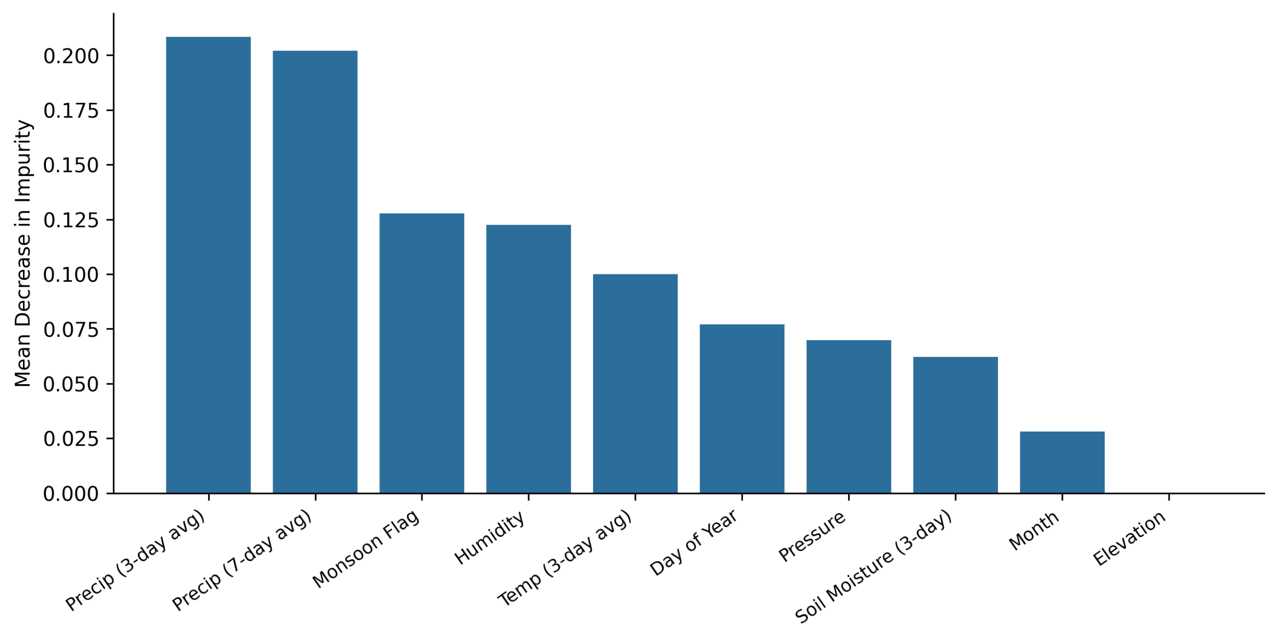
Feature-importance analysis identified the 3-day and 7-day precipitation averages, the monsoon indicator and humidity as the leading predictors. Soil moisture and atmospheric pressure had lower importance in the fitted model, as shown in Figure 1.

Visual Patterns in the Data

The 2022 Flood Season

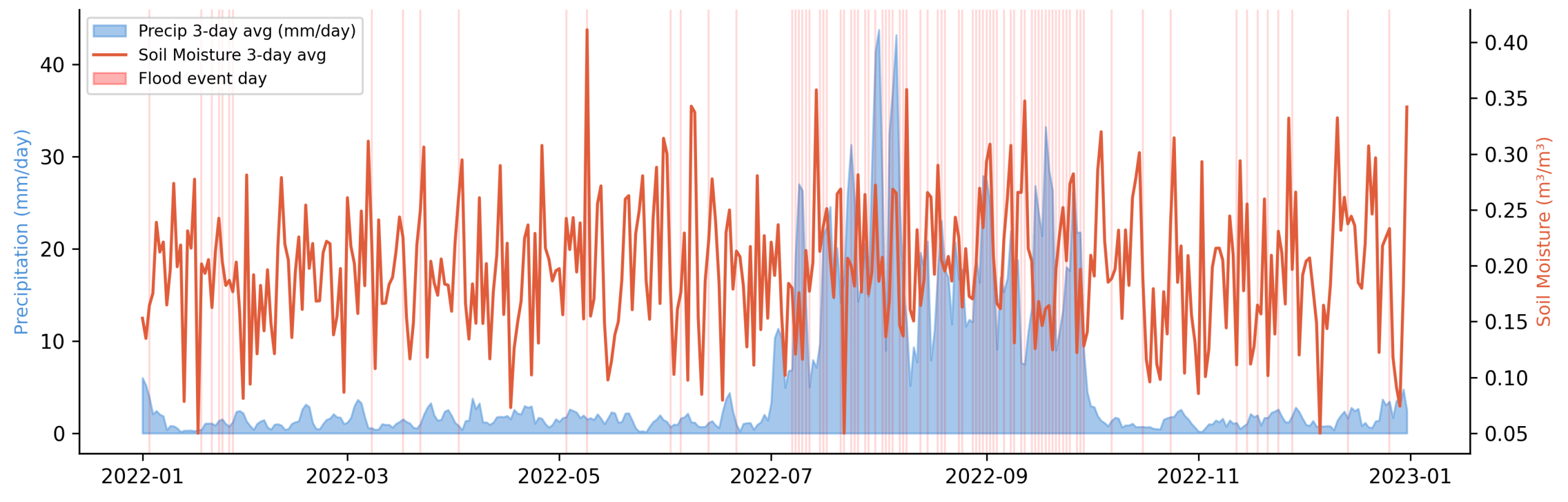
In the 2022 monsoon time series we observe the anticipated order of rainfall intensifying, soil moisture reacting and then the flood-event labels taking place most often when both signals are elevated. “It’s not a perfectly neat pattern and that’s helpful.” It demonstrates the necessity of lagged and rolling variables in the model, not just a single same-day rainfall value.

Precipitation and Soil Moisture

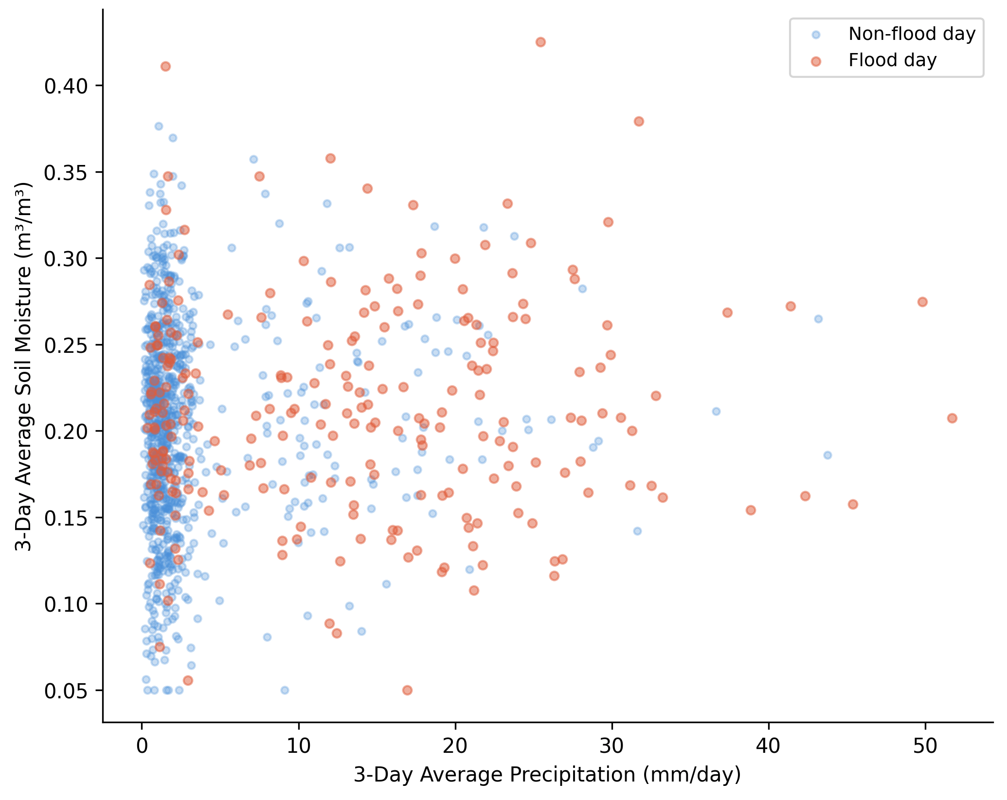
The scatter plot shows substantial overlap between the two classes. Flood-event days occur more frequently at higher precipitation values, but precipitation and soil moisture do not provide perfect separation. This is hydrologically plausible because flooding also depends on timing, drainage, antecedent conditions and label uncertainty. It also explains why the threshold model was useful as a baseline but insufficient as a final classifier.

Precipitation Density

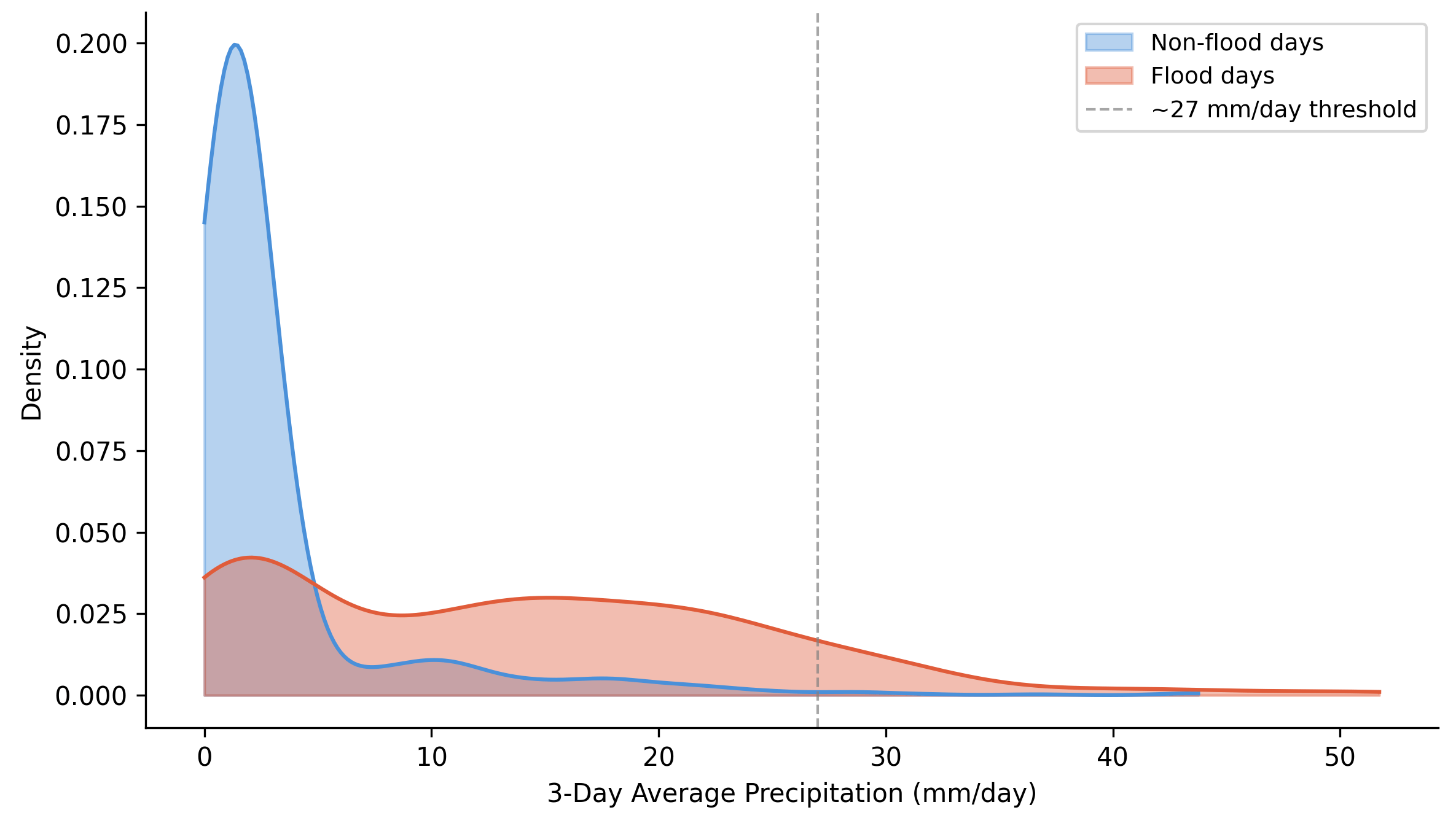
The density plot quietly says the same thing. Flood days move to higher 3-day precipitation, especially around the 25-30 mm/day range, but the two curves still overlap. The rain helps, it doesn’t win the case on its own.

Monthly Flood Frequency

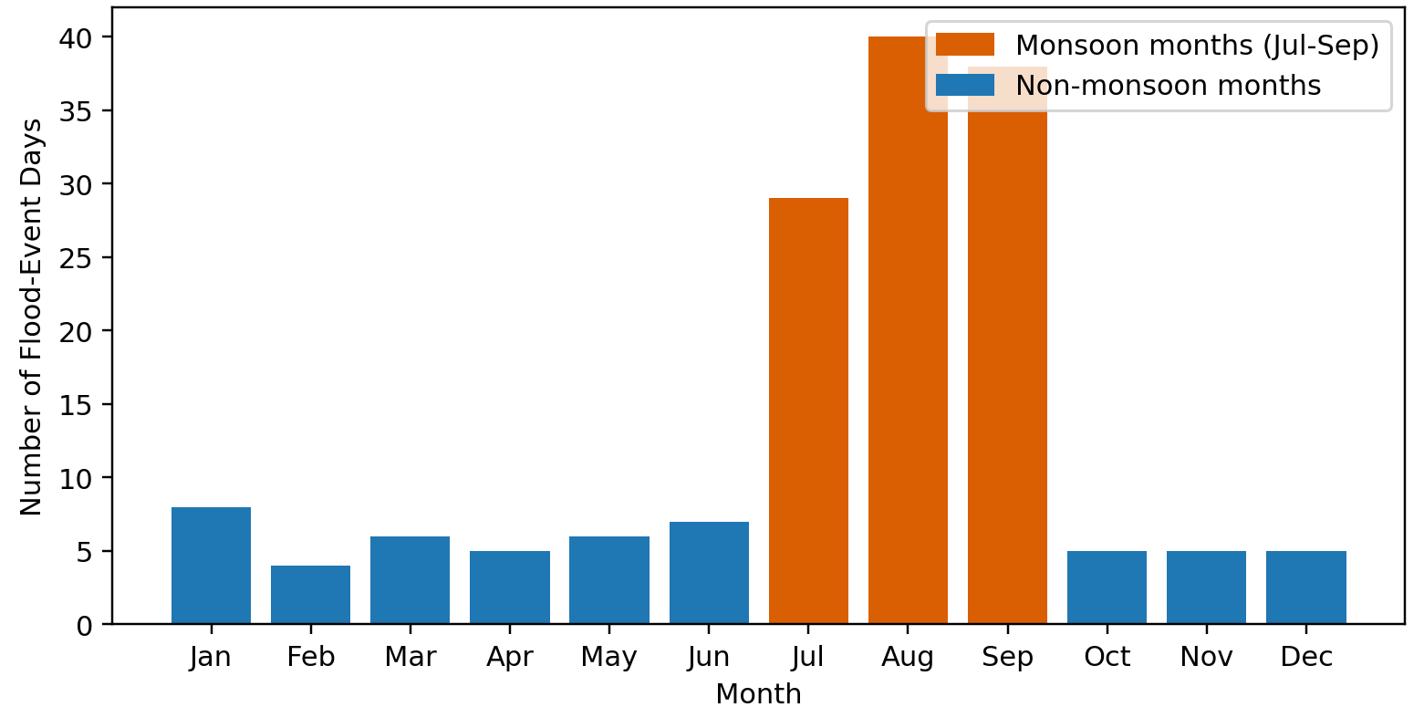
The plot for the month is almost too obvious: most of the flood days we labeled fall in July, August, and September. This is consistent with the southwest monsoon and not surprising but it sets up a modeling pitfall. A classifier might seem smart because it learns the calendar. That may be partly legitimate for Dadu, but much less so for another district, or for a strange year.

Correlation Structure

The 3-day and 7-day precipitation averages and the monsoon indicator show the strongest positive correlations with the flood-event label. Humidity shows a moderate positive relationship, while soil moisture has only a weak direct correlation in this dataset. Atmospheric pressure shows a modest negative relationship.

Discussion

The following is an explanation of what the Performance Results mean: It’s not the 77.3% accuracy but the recall problem that’s most important. The model identified only 50% of flood-event days in the random split and fewer than 50% in the temporal split. This performance may be informative for an exploratory classification study, but it is insufficient for operational early warning. Nevertheless, the experiment identified flood-related signals in rainfall, soil wetness and seasonality. The limitation is that these signals were not converted into sufficiently reliable warnings.

Why False Negatives Matter More than False Alarms

There are different consequences associated with the two types of flood-warning error. If a false alarm occurs too frequently it can lead to lack of confidence in the public and/or cause unnecessary movement and wasted time. A missed flood is a different story: People may be totally unaware of an impending flood to roads, homes, livestock, or stored food. In such a context recall is not just one of the numbers in a table, but it is linked to the function of the model. There are some modifications which can help the model to achieve a higher level of recall. The easiest thing would be to turn that to less than 0.5, and allow more false alarms. A cost sensitive loss or boosted-tree model may be useful as well; XGBoost demonstrated a slight improvement in the flood recall in the baseline comparison. If the key signal is the slow accumulation of rainfall and soil moisture over several days, then a sequence aware model might be required. I think that the threshold change is worth trying first; it doesn’t require any new data, no cost, and the result of XGBoost gives a sense that it should be possible to do better with respect to recall without redoing the work.

Generalizability Beyond Dadu

The outcomes ought to remain connected to Dadu. The nature of the flood geography of Pakistan is so varied that a model which is applicable to one district cannot be considered as a national model. The glacier-fed rivers and flash regime of KPK is hardly recognizable to the flat alluvial terrain of Dadu. Even in Sindh a district even further upstream would act differently. Back to the Balochistan and Punjab flood mechanisms again and there is no short-cut in this regard to test it in those areas before making the overall claims. A more robust subsequent study would have trained and tested within districts. Some districts should be excluded from training and the model should be presented with districts that it has not encountered before. That design would indicate if the predictors are learning to predict transferable flood processes or the “local ways” of one record. Atmospheric pressure showed a modest negative association with the flood-event label and lower feature importance than the leading precipitation and seasonal variables. It may partly reflect broad monsoon circulation, but the short three-year record makes it difficult to determine whether pressure is a stable physical predictor or a seasonal proxy. A longer record, including atypical monsoon years, would be needed before interpreting it as a consistent predictor.

Dataset Limitations

The problem studied has a small-size dataset. It lasts for 730 days, and 158 flood event days. The record includes extreme flood conditions, particularly during 2022, which may cause the model to represent severe events better than more moderate flood years. But, there’s a question about labels themselves that I’m less able to resolve. The uncertainty is not only in the inundation prediction by the model, but also during heavy monsoon cloudy days, MODIS based inundation estimates are not certain, and some true flood days may not have been labeled in the process. Not that that makes the data set obsolete, but this is not the same type of uncertainty that is associated with missing predictor values, and it should be identified. The extension of the record would help, but isn’t as easy. A 2010-2024 record would contain the record of the 2010 super-floods and more of the variations in monsoon behavior. The challenge here is that the data on SMAP starts in 2015, meaning that prior years would need to be supplied with different sources of soil moisture, like ERA5-Land and/or ASCAT. This would have to be proven as a separate replacement.

Satellite-Data Uncertainty

The open-data approach is appealing as it can be applied in areas with a lack of local instruments. The same might be a disadvantage, too. Monsoon cloud cover limits MODIS observations; Integrated Multi-satellitE Retrievals for GPM (IMERG) may miss or smooth some extreme precipitation; and SMAP has limitations over very wet or complex surfaces. It does not imply that the results are to be used as a precise value but should be used as a cautious approximation. When writing a research paper, it’s sufficient to report those limitations. They would have to be dealt with directly in a warning system, both via uncertainty measures and through comparison with local observations, and via methods of communicating confidence to decision makers.

Operational Readiness

The model is not yet able to be used for issuing a warning to the public for flooding events. Recall is still low, validation is still too limited and the flow is not yet linked to real-time delivery of data or to government decision making. Issuing SMS alerts at this stage would create an appearance of operational readiness that the available evidence does not support. A responsible deployment pathway would first improve recall under temporal validation, test the model across several districts, establish a real-time data pipeline and consult NDMA, provincial authorities and local officials about whether the warnings would meaningfully support decisions on the ground. Public deployment should only be considered after these steps. Then, public use would be a topic of discussion.

Conclusion

The most salient take away from this pilot is that although open data can take a flood model quite a bit, it may not be enough to reach operational use. Based on GPM IMERG, SMAP, ERA5, elevation and rolling features, a daily flood-event classifier was created for Dadu district from 2022-2024. Although the time series was small (730 days, with 158 flood event days), some identifiable relationships were found between the rainfall, soil wetness, pressure, seasonality and flood labels. The lack of translation to those links meant that there was not sufficient recall. Random Forest was able to achieve 77.3% accuracy on a random split but only obtained 50% of the flood days. The more realistic temporal test resulted in a decrease to 44% of recall. This alters the meaning in the work. This is not an alarm system, it’s a careful first model. The contribution is not so dramatic, but rather practical. The paper provides a repeatable district-level process, a comparison to baselines, illustrates the variables the model used and makes the recall problem apparent. This is important for a hazard such as flooding. It is better to have an accurate weak model than an impressive one that is over-described. Future work should begin with the “missed events”, and not with a larger claim. The first thing that should improve is the recall; likely through threshold tuning or gradient boosting; if the lag structure of the figures is real, then a temporal model deserves a serious test as well. The record should be expanded to include additional years and districts as well. Otherwise it would continue to be hard to determine if the model has learned flood processes or just the way this short Dadu record works. If the steps are successful, then open-data modeling can help in preparedness planning within rural Pakistan. It remains unclear how far a satellite-only approach can progress before local observations become essential. At present, the evidence supports a cautious conclusion: useful flood-related signals are present, but the model is not operationally ready.

Data Availability Statement

The public datasets were analysed. NASA Earthdata offers GPM IMERG precipitation data; the National Snow and Ice Data Center offers the SMAP Level-4 soil moisture data; the ECMWF Copernicus Climate Change Service offers ERA5 reanalysis data; and the United States Geological Survey (USGS) EarthExplorer offers SRTM elevation data. The cleaned daily dataset and Python scripts are not included with the manuscript but are available from the corresponding author upon reasonable request. 

References

1. World Bank. Pakistan: flood damages and economic losses over USD 30 billion and reconstruction needs over USD 16 billion. World Bank Press Release, 2022, https://www.worldbank.org/en/news/press-release/2022/10/28/pakistan-flood-damages-and-economic-losses-over-usd-30-billion. [↩]
2. UNOCHA. Pakistan: 2024 floods extent statistics, 21 August 2024. United Nations Office for the Coordination of Humanitarian Affairs, 2024, https://www.unocha.org/publications/report/pakistan/pakistan-2024-floods-extent-statistics-21-august-2024. [↩]
3. M. S. Tehrany, B. Pradhan, M. N. Jebur. Flood susceptibility analysis and its verification using a novel ensemble support vector machine and frequency ratio method. Stochastic Environmental Research and Risk Assessment. Vol. 29, pg. 1149-1165, 2015, https://doi.org/10.1007/s00477-015-1021-9. [↩]
4. K. Khosravi, E. Nohani, E. Maroufinia, H. R. Pourghasemi. A GIS-based flood susceptibility assessment using statistical and ensemble modeling approaches. Stochastic Environmental Research and Risk Assessment. Vol. 30, pg. 2085-2100, 2016, https://doi.org/10.1007/s00477-016-1271-6. [↩]
5. M. Khan, A. U. Khan, B. Ullah, S. Khan. Developing a machine learning-based flood risk prediction model for the Indus Basin in Pakistan. Water Practice and Technology. Vol. 19, pp. 2213–2225, 2024. https://doi.org/10.2166/wpt.2024.151. [↩]
6. M. Waleed, M. Sajjad. High-resolution flood susceptibility mapping and exposure assessment in Pakistan: An integrated artificial intelligence, machine learning and geospatial framework. International Journal of Disaster Risk Reduction. Vol. 121, Article 105442, 2025. https://doi.org/10.1016/j.ijdrr.2025.105442. [↩]
7. M. Waleed, M. Sajjad. Advancing flood susceptibility prediction: A comparative assessment and scalability analysis of machine learning algorithms via artificial intelligence in high-risk regions of Pakistan. Journal of Flood Risk Management, 2025. https://doi.org/10.1111/jfr3.13047. [↩]
8. H. He, E. A. Garcia. Learning from imbalanced data. IEEE Transactions on Knowledge and Data Engineering. Vol. 21, No. 9, pp. 1263–1284, 2009. https://doi.org/10.1109/TKDE.2008.239. [↩]
9. M. Sit, B. Z. Demiray, Z. Xiang, G. J. Ewing, Y. Sermet, I. Demir. A comprehensive review of deep learning applications in hydrology and water resources. Water Science and Technology. Vol. 82, pg. 2635-2670, 2020, https://doi.org/10.2166/wst.2020.369. [↩]
10. G. J. Huffman, E. F. Stocker, D. T. Bolvin, E. J. Nelkin, J. Tan. GPM IMERG Final Precipitation L3 1 day 0.1 degree x 0.1 degree V06. Goddard Earth Sciences Data and Information Services Center, 2020, https://doi.org/10.5067/GPM/IMERGDF/DAY/06. [↩]
11. D. Entekhabi, E. G. Njoku, P. E. O’Neill, K. H. Kellogg, W. T. Crow, W. N. Edelstein, J. K. Entin, S. D. Goodman, T. J. Jackson, J. Johnson, J. Kimball, J. R. Piepmeier, R. D. Koster, N. Martin, K. C. McDonald,M. Moghaddam, S. Moran, R. Reichle, J. C. Shi, J. J. Van Zyl. The Soil Moisture Active Passive (SMAP) mission. Proceedings of the IEEE. Vol.98, pg. 704-716, 2010, https://doi.org/10.1109/JPROC.2010.2043918 [↩]
12. A. Younas, A. Khan, H. M. Abubakar, Z. Tahseen, A. Arshad, M. Taj, U. Nazir. 2022 Flood Impact in Pakistan: Remote Sensing Assessment of Agricultural and Urban Damage. arXiv:2410.07126, 2024. https://arxiv.org/abs/2410.07126. [↩]
13. S. Nevo, E. Morin, A. Gerber Anner, A. Metzger, C. Kim, C. Librescu, G. Nearing, Y. Matias. Flood forecasting with machine learning models in an operational framework. Hydrology and Earth System Sciences. Vol. 26, pg. 4013-4032, 2022, https://doi.org/10.5194/hess-26-4013-2022. [↩]