DiaBreath: Multivariate Analysis of a Non-Selective Low-Cost Metal Oxide (MOX) Sensor Array for Breath-Based Diabetes Screening

Abstract

The number of diabetes patients is increasing worldwide, but many cases stay undiagnosed in low-resource regions. The A1C blood test is invasive and costly, therefore it is often not available in these regions. In this research, DiaBreath is proposed as a low-cost noninvasive screening system based on exhaled breath analysis. Volatile organic compounds (VOCs) in breath are measured with an array of MQ-series gas sensors. They are inexpensive but non-selective, so a single sensor cannot distinguish one VOC from another. To solve this, multivariate analysis was applied to the sensor array responses, including principal component analysis (PCA), Random Forest classification, and partial least squares (PLS) regression. In the PCA result, six VOCs formed separate clusters, and the Random Forest classifier showed an accuracy of 0.83. The PLS model estimated the acetone concentration with an R² of 0.98 and an RMSE of 8.77 ppb, and it followed the GC-MS reference with an R² of 0.9900 from 50 ppb to 5 ppm. For diabetes screening, an XGBoost model was trained on a synthetic breath VOC dataset, and it showed a test ROC-AUC of 0.9861. The trained model was embedded into a portable Arduino-based device that connects to a mobile application through Bluetooth. Since the model was trained on synthetic data, the result is closer to a feasibility check than a clinical test. These results showed that a low-cost MQ sensor array with multivariate analysis can be used for noninvasive diabetes screening.

Keywords: Diabetes diagnosis, Volatile organic compounds, Gas sensor array, Multivariate analysis, Machine learning, Noninvasive screening

Introduction

Early detection of diabetes is crucial to prevent permanent life-threatening damage. Current methods to diagnose diabetes such as the A1C blood test are invasive and often financially and environmentally limited¹. This creates difficulties in rural and developing communities, often leading to serious health concerns that are irreversible. Undiagnosed diabetes mellitus (UDM) is a serious concern in modern healthcare, with estimates of over 175 million UDM cases existing, an estimated 83.8% of which are from the low- and middle-income classes². According to Saydah et al., there is a direct correlation between economic status and diabetic mortality³. Having a family income below the poverty line was associated with a twofold higher diabetic mortality rate than that of the upper class³. In summary, there needs to be a low-cost and noninvasive method to screen for diabetes, to help reduce UDM around the world.

Breath analysis has become one of the promising non-invasive methods for several diseases⁴. For diabetes, the most studied breath biomarker is acetone⁴. When the body does not have enough insulin, it starts to burn fat instead, and this produces ketone bodies. Acetoacetate from this process breaks down into acetone on its own, and the acetone comes out in the breath⁵. Studies that used gas chromatography-mass spectrometry (GC-MS), proton-transfer-reaction mass spectrometry (PTR-MS), or selected-ion flow-tube mass spectrometry (SIFT-MS) have reported that breath acetone is higher in diabetic patients, around 2 ppm in type 2 diabetic patients while healthy people are around 0.5 ppm^6,7,8. But these instruments cost from tens of thousands to over a million dollars each, so they are not really suitable for screening many people or for point-of-care use⁹.

To make breath screening cheaper and more accessible, two directions have been tried so far^10,11. The first one is to make sensing materials that are highly selective to acetone, like Si-doped WO₃ nanoparticles¹⁰. The second one is to use an array of low-cost, non-selective metal oxide (MOX) gas sensors together with machine learning, so that the selectivity is recovered from the overall response pattern instead of the material itself¹¹ Recent low-cost e-nose studies in this second direction reported accuracies from about 87% to 100%, on groups of about 44 to 1,000 people^12,13,14,15. These include an MQ-array system by Gudiño-Ochoa et al.¹² that runs the model with TinyML, a method for deploying lightweight machine learning models on small low-power devices12, an in-car e-nose by Weng et al.¹³, a SAW-based device by Bahos et al.¹⁴, and a Figaro TGS-array system tested on a larger group by Taspinar¹⁵.

These studies show that low-cost MOX arrays can tell diabetic and non-diabetic breath apart. However, in most of them the sensor array is just used as a black-box input for the classifier. Whether the array itself can actually separate individual VOCs or estimate their concentrations through multivariate analysis is usually not checked. In other words, it is still not clear how much VOC-specific information a cheap non-selective array can recover on its own, compared to selective materials or expensive instruments.

This study looks at this gap in two steps. First, the response of a non-selective low-cost MOX sensor array is analyzed using a public multi-VOC dataset^16,17. PCA (principal component analysis), Random Forest classification, and PLS (partial least squares) regression are applied to check whether the array can separate six different VOCs and estimate acetone concentration without any selective material. To see how reliable these concentration estimates are, the PLS predictions are also compared against GC-MS measurements, which is used here as a reference method. How the sensor array responds across different concentration levels is also examined, since MOX sensors are known to be nonlinear. Second, the same approach is extended to breath-based diabetes screening with a public synthetic breath VOC dataset⁶, and the trained model is put on an Arduino-based portable device that connects to a mobile application through Bluetooth. The device is presented as a feasibility-stage prototype. Combining it with patient-reported risk factors and testing it on real diabetic breath are left as future work.

Methods

Datasets

This study used two datasets, and both are publicly available. No human subjects were recruited.

The first one is the Gas Sensor Array Low-Concentration dataset from the UCI Machine Learning Repository^16,17. We used it for the multivariate analysis described below. It has the responses of a 10-channel MOX sensor array to six VOCs. The six are ethanol, acetone, toluene, ethyl acetate, isopropanol, and n-hexane. Each gas was measured at 50, 100, and 200 ppb, and five samples were taken for each gas at each concentration, so there are 90 samples in total. One thing to note is that these concentrations are all at the ppb level. This is lower than the acetone level that diabetic breath usually shows¹⁸, which is around the ppm range. So we used this dataset to check whether the array can tell the six gases apart, not to copy real breath conditions. Also, the 10 sensors are not only MQ sensors. Some of them are Figaro TGS sensors.

The second one is a synthetic breath VOC dataset from Gudiño-Ochoa et al.¹². This was used to train the breath-based diabetes screening model described later. They first collected real breath data from a small number of people, and then used a generative model called CTGAN (Conditional Tabular Generative Adversarial Network) to make 14,000 synthetic samples out of it. Their device uses an MQ sensor array and raw value of each sensor, so we kept the same sensor types and the same output format to make the input match. But matching the sensor types does not really mean the response distribution becomes the same, and this point is discussed later as a limitation in the discussion. Since this dataset is synthetic and not from real patients, the screening result is closer to a feasibility check than a clinical test.

The synthetic breath VOC dataset was split into train and test sets with an 8:2 ratio. Stratified sampling was used so that the class ratio stays the same, and the random seed was fixed to 42. 5-fold stratified cross-validation was applied during training (see the Breath VOC Screening Model section). We also made a correlation matrix for the breath VOC dataset before training. This was just to check how each sensor variable is related to the diabetes label.

This study only used public and anonymized datasets, and no data was collected from human subjects, so IRB approval was not needed. For the hardware tests described later, no human breath was used either. The device was checked only with reference gas samples.

Multivariate Analysis of the MOX Sensor Array

The MOX sensors used for this analysis are non-selective, so it is hard to identify a specific VOC or measure its concentration with a single sensor¹⁹. This is because each sensor responds to multiple gases at the same time, and a single sensor output is not enough to tell apart different VOCs in human breath, which contains many volatile compounds at once. To solve this problem, an array of multiple sensors is used. Each sensor has a slightly different sensitivity pattern, and these patterns can be combined using multivariate analysis to extract more information about the VOCs²⁰. For this purpose, the UCI Gas Sensor Array Low-Concentration dataset described above was used to perform PCA, Random Forest classification, and PLS regression.

Since MOX sensors are not selective, the output of one sensor reflects the combined response from multiple VOCs, not a single chemical. This can be expressed as:

   

Here, is the output of the -th sensor, is the true concentration of VOC , is the sensitivity of sensor to VOC , and is an error term that includes environmental noise such as temperature and humidity. This linear form is only an approximation, since MOX sensors are actually nonlinear and humidity-dependent, but it is used here to explain the basic idea behind the array. If we assume there are sensors in total, the equation can be written in matrix form as:

   

is the sensor sensitivity matrix, where each row shows the sensitivity profile of one sensor. When the sensors have different sensitivity patterns, the rows of point in different directions, and the rank of the matrix becomes higher. A higher rank means the sensor array gives more independent information, which makes it easier to tell different VOCs apart using multivariate methods. In this sense, the non-selectivity of each sensor is not only a drawback, because as long as the sensors are non-selective in different ways, the array as a whole carries more information.

To check whether the sensor responses can be separated by VOC type, PCA was applied to the sensor response matrix . PCA finds the main directions of variance by performing eigenvalue decomposition on the covariance matrix:

   

Where M is the total number of samples, Q=[q_1,q_2,…] contains the principal component directions, and Λ=diag(λ_1,λ_2,…) contains the eigenvalues, which show how much variance each component explains. The principal components (PCs) were then used to see how clearly the sensor responses for different VOCs are separated in high-dimensional space.

If different VOCs or concentrations show different response patterns, they will form separate clusters in the PCA space.

For estimating concentration, PLS regression was used. PLS finds latent directions that maximize the covariance between the sensor response matrix and the target concentration vector :

   

where is a weight vector that projects the sensor responses into a latent space. The latent variable

   

is built so that it has a strong linear relationship with VOC concentration. The final prediction model is:

   

where is the predicted VOC concentration and is a regression coefficient vector trained to fit the linear relationship between the latent variables and the target concentrations.

To check whether the predicted concentrations are accurate or not, the PLS predictions were compared with GC-MS results, which was used as the reference method. Certified acetone standard gas was diluted with high-purity nitrogen into seven concentrations, which were 50, 100, 200, and 500 ppb, and 1, 2, and 5 ppm, regarding the UCI dataset range and actual acetone concentration found in diabetic breath¹⁸. For each concentration of gas, the standard acetone gas was filled into a 1 L Tedlar bag (Thermo Scientific CP8656100). Then, one aliquot was taken from the bag for GC-MS analysis. Right after that, the DiaBreath device was exposed to the gas from the same bag. This way, both measurements come from the same sample. The R_s/R₀ values from the MOX-based device were put into the PLS model to predict the concentration. This predicted value was then compared with the GC-MS result.

The device measurement followed a fixed protocol for each sample. First, the sensors were given a warm-up time of 10 min. After that, the device was kept in air for 5 min to stabilize, and the baseline resistance R₀ was taken as the average of the last 60 s in air. Then the device was exposed to the standard gas for 3 min, and the R_s/R₀ value was taken as the average of the last 60 s of this exposure. After each measurement, the device was purged with air for 10 min before the next sample. Each concentration was measured three times (n = 3).

The GC-MS analysis was held by Thermo Fisher Scientific TRACE 1310 GC coupled with ISQ QD300 single quadrupole MS and TriPlus RSH SMART autosampler. TraceGOLD TG-5MS column was used, which is a low-polarity column made of 5% diphenyl and 95% dimethyl polysiloxane. For each sample, 1.0 mL of gas was injected in splitless mode, and the inlet was kept at 220°C. The carrier gas was helium (99.999%) at a constant flow of 1.0 mL/min. The oven started at 40°C and was held for 5 min. Then it was ramped at heating rate of 20°C/min up to 200°C and held there for 2 min. For the MS, Electron Ionization (EI) was used at 70 eV. The ion source was kept at 230°C, and the transfer line at 200°C. A full scan from m/z 35 to 400 was used to confirm acetone. For quantification, SIM mode was used. In this mode, m/z 43 was the quantifier ion and m/z 58 was the qualifier ion²¹. The acetone concentration was calculated from an external calibration curve, based on the peak area of m/z 43²¹.

Since the seven concentrations cover a wide range from 50 ppb to 5 ppm, the sensor responses can also be checked for nonlinearity over this range. The R_s/R₀ values were plotted against concentration to see whether the response stays linear or becomes saturated at higher concentrations, and the residuals between the PLS predictions and the GC-MS values were examined to see if the prediction error depends on concentration.

Breath VOC Screening Model

Before building the device, the screening model has to be trained with the breath VOC data. Each model takes the breath VOC data as input, and outputs a probability of whether the input is diabetic or not. As mentioned above, the data was split into train and test sets with an 8:2 ratio, using stratified sampling and a random seed of 42.

Four models were tested on the breath VOC data: XGBoost, LightGBM, Random Forest, and logistic regression. XGBoost and LightGBM are both gradient boosting methods, and the main difference is just how they grow the trees, with LightGBM being lighter and faster^22,23. Random Forest is a bagging method that uses many decision trees and takes a majority vote²⁴. Logistic regression was put in as a simple baseline, since it is easy to interpret and works fine when the relationship is close to linear.

Then, a 5-fold stratified CV (cross-validation) was also applied so that the results would not depend too much on a single random split.

Hyperparameters of each model were tuned using a grid search algorithm. For XGBoost, the search range was max_depth ∈{3,5,7}, learning_rate ∈{0.01,0.1,0.3}, and n_estimators ∈{100,200,500}. For LightGBM, num_leaves ∈{31,63,127}, learning_rate ∈{0.01,0.1}, and n_estimators ∈{100,200,500} were searched. For Random Forest, n_estimators ∈{100,200,500}, max_depth ∈{None,10,20}, and min_samples_split ∈{2,5,10} were searched. The combination with the highest mean ROC-AUC score from CV was selected as the final hyperparameter set for each model.

All four models were trained on the breath VOC data and compared by their ROC-AUC values. The model with the highest test ROC-AUC was selected as the final model for the breath VOC data. The detailed comparison is presented in the Results.

Hardware Construction

The gas sensors used in DiaBreath consist of five MQ-series sensors (MQ-2, MQ-3, MQ-7, MQ-135, MQ-138) and one SGP-30 MOX sensor from Sensirion (Figure 1a). Each sensor was selected to cover a different range of VOCs that are relevant to diabetic breath²⁵. MQ-2 responds to LPG, hydrogen, methane, and smoke; MQ-3 responds to alcohol and benzene; MQ-7 responds to carbon monoxide; MQ-135 responds to ammonia, NOx, alcohol, benzene, and CO2; and MQ-138 responds to acetone, formaldehyde, alcohol, and toluene. The SGP-30 was added to measure total VOCs (TVOC) and ethanol, which provides additional information that the MQ sensors cannot resolve on their own. The combination of these six sensors provides overlapping but partially distinct sensitivity patterns, which is the basis for the multivariate analysis described above.

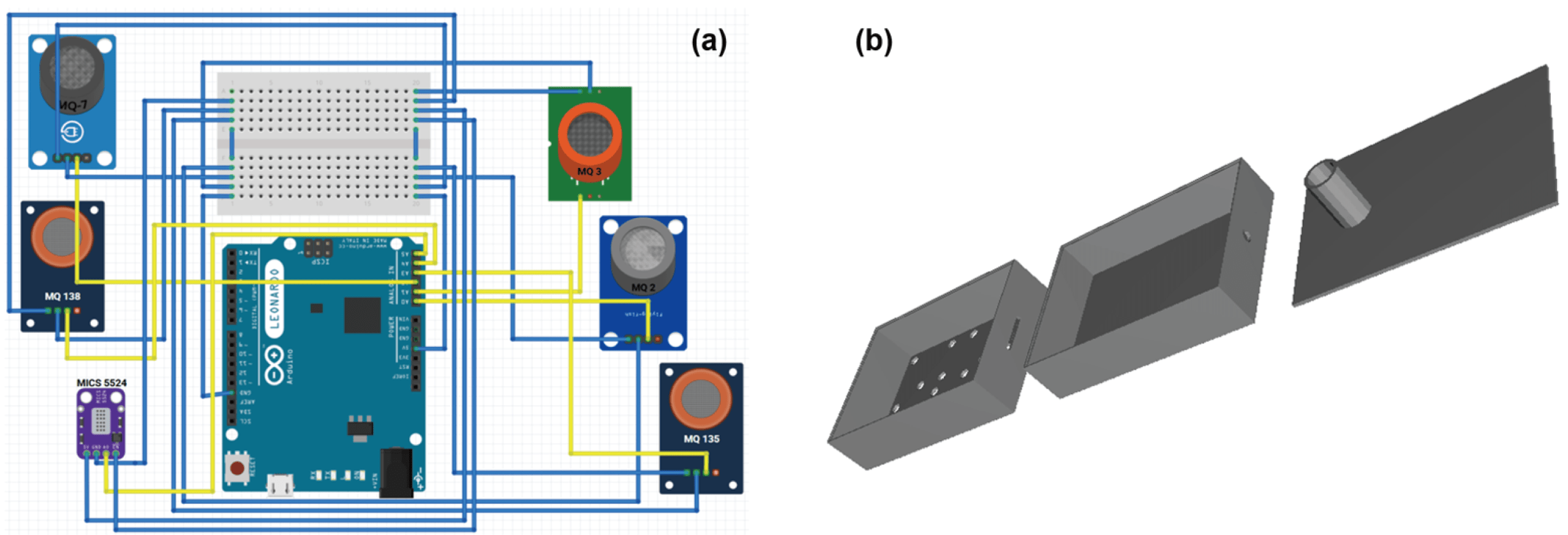
Among these sensors, four of them (MQ-2, MQ-3, MQ-135, MQ-138) match the sensor types used in the synthetic breath VOC dataset, so the screening model can take their R_s/R₀ values as input. MQ-7 and the SGP-30 were added as extra sensors for more VOC coverage, but they are not part of the training data. This mismatch between the hardware sensors and the training data is a limitation, and it is discussed further in the Discussion.

The sensors are connected to a breadboard, which is connected to the Arduino Leonardo’s 5V and GND pins, and the analog pins are connected directly to the Arduino. The whole apparatus is placed inside a hand-holdable shell that was modeled in Fusion 360 and 3D printed with PLA (Figure 1b). After the screening model was trained, it was embedded into the device. During a measurement, the Arduino reads the output value of each sensor on its analog pin and sends these values to a smart device. The measurement protocol, including the warm-up and sampling steps, is described above in the Multivariate Analysis section.

A smart device application was created so that the device can be used without a computer. The data is sent wirelessly through an HM-10 Bluetooth module to the application, which then runs the trained model on the received sensor values. This is an improvement over the earlier version, which sent the data to a computer through a cable and a serial port, since the new version is wireless and easier to use.

Results

Correlation Analysis of VOC Sensor Responses

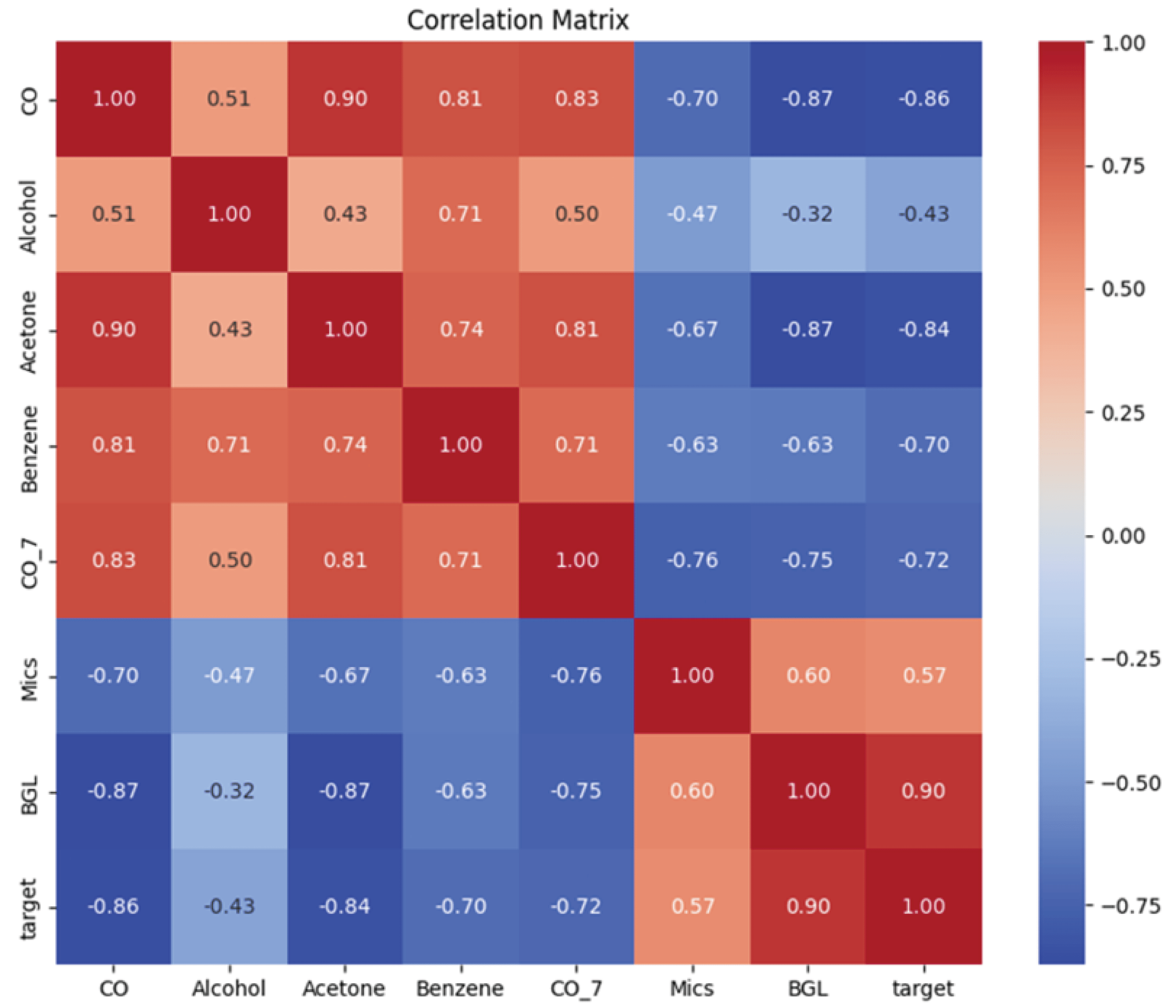
The correlation matrix of the breath VOC dataset (Figure 2) shows strong negative correlations between diabetes and CO (−0.86), and between diabetes and acetone (−0.84). This matches the known trend from earlier studies, where diabetic breath tends to contain more ketones and CO because of the metabolic changes in diabetes²⁶. However, since this dataset is synthetic and was generated from earlier experimental data, this result mainly shows that the synthetic data keeps the same trend as the original data, rather than confirming the biology on its own. Most of the sensor variables show negative correlations with diabetes. This is because each sensor returns the R_s/R₀ value, which decreases as more of the target VOC is detected, so a higher VOC concentration gives a lower sensor output. The strong negative correlations of CO and acetone suggest that the MOX sensor array picks up the VOC differences related to diabetes.

Multivariate Analysis of VOC Sensor Responses

The response patterns of the MOX sensor array were collected from six different VOC samples and projected into a low-dimensional space using PCA (Figure 3). Each VOC formed a clearly separated cluster in the PC1-PC2 space. Although the MOX sensors are non-selective, the six VOCs did not overlap with each other, which means the sensor array still produces VOC-specific patterns when the responses are combined.

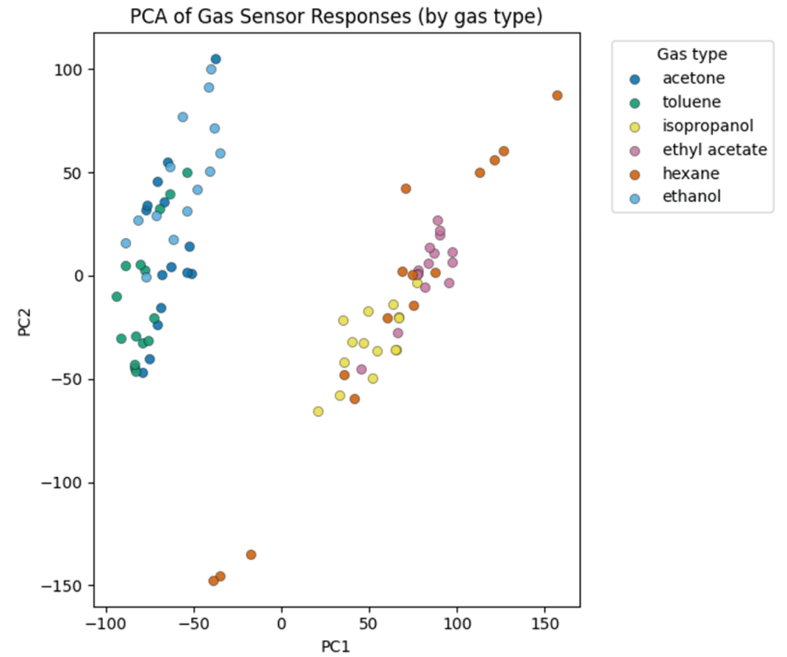
The PC1 axis mainly reflects the overall response size of the sensor array and how each VOC reacts differently with the sensor surface. This is because MOX sensors work through oxidation-reduction reactions and surface adsorption, and the strength of these reactions changes with the type of VOC. The PC2 axis reflects more detailed differences, such as how much each individual sensor contributes to the response or how electron transfer differs between VOCs. Both axes show clear separation between VOCs, which means the sensor responses contain enough statistical information to tell different VOCs apart.

Oxygenated VOCs such as ethanol, isopropanol, and acetone formed separate clusters even though they have similar chemical structures. Nonpolar VOCs such as hexane and toluene also appeared as their own clusters. This suggests that the sensor array responses reflect physical and chemical properties of the gases, including polarity, molecular weight, and how strongly each VOC interacts with the metal oxide surface. These results show that array-based multivariate analysis can tell apart VOCs that single-sensor signals cannot.

To check whether the sensor array can classify different VOC types, a Random Forest model was trained on the multisensor responses (Table 1). The overall classification accuracy was 0.83, which shows that the model learned the differences between VOC response patterns even though the MOX sensors are non-selective. Hexane and toluene showed perfect classification with precision, recall, and F1-scores of 1.00, which means these two VOCs have very distinct response patterns. On the other hand, ethanol, ethyl acetate, and isopropanol showed lower F1-scores between 0.67 and 0.80. This is because ethyl acetate and isopropanol have similar sensitivity profiles across multiple sensors, so their multivariate patterns partially overlap. This is consistent with the incomplete separation seen in the PCA plot.

Gas type	Precision	Recall	F1-Score
Acetone	0.75	1.00	0.86
Ethanol	1.00	0.67	0.80
Ethyl acetate	0.67	0.67	0.67
Hexane	1.00	1.00	1.00
Isopropanol	0.67	0.67	0.67
Toluene	1.00	1.00	1.00

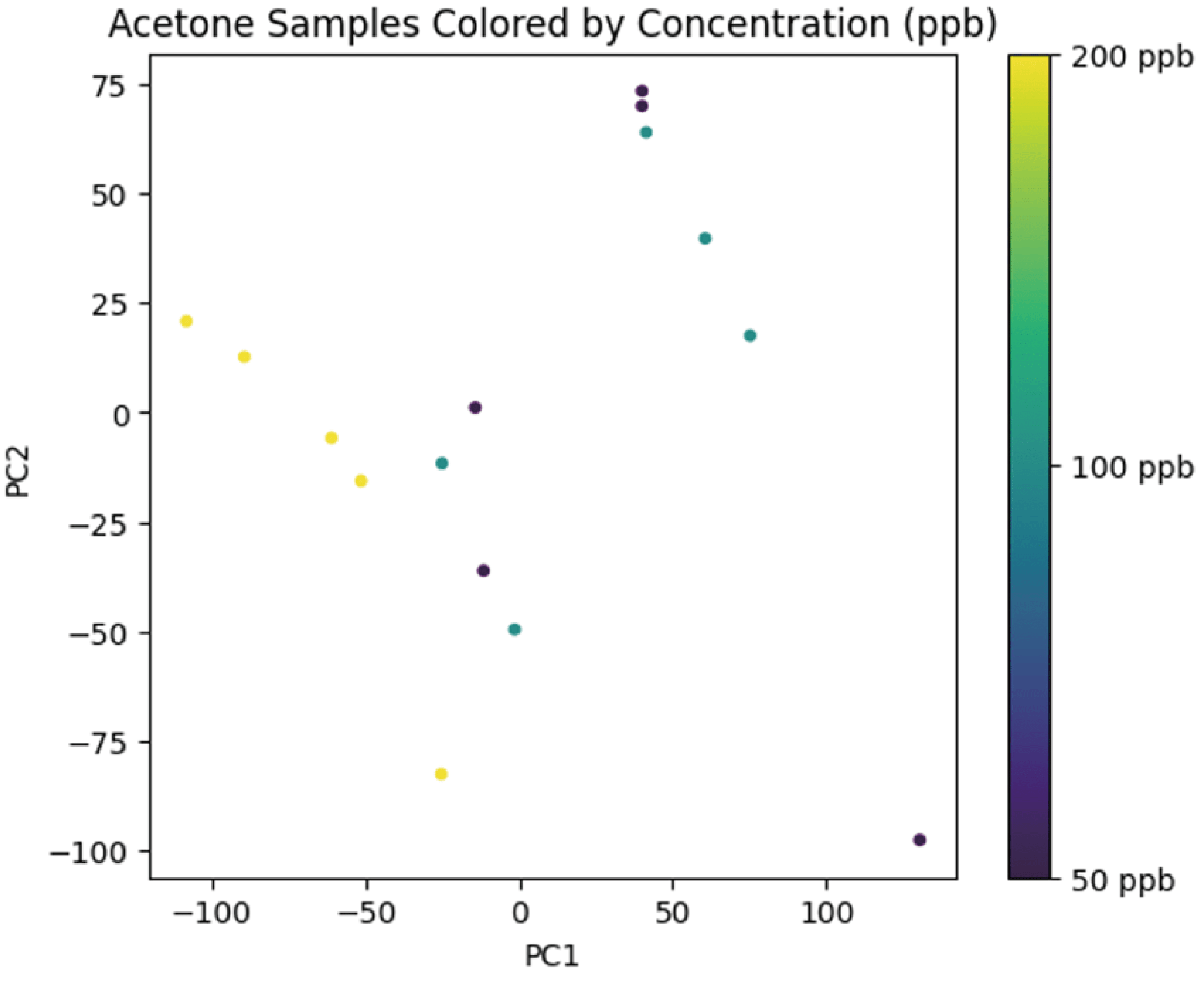
The concentration-dependent behavior of sensor responses was analyzed using acetone samples at different concentrations between 50 and 200 ppb (Figure 4). The center of the data distribution gradually shifted in the PCA space as concentration increased. High-concentration samples (200 ppb) were located in lower PC1 regions, while low-concentration samples (50 ppb) spread out toward higher PC1 and PC2 regions. This shows that the response patterns change in a structured way with concentration. At the same time, samples at the same concentration did not collapse into a single point but spread out a little in the PCA space. This spread comes from the nonlinear response of MOX sensors, sensor-to-sensor variation during repeated measurements, and small changes in environmental conditions.

To estimate the concentration of a single VOC from multisensor responses, PLS regression was applied to the acetone samples. The trained PLS model achieved an R₂ value of 0.98 on the UCI dataset, which means about 98% of the variance in true acetone concentrations was explained by the model. The RMSE was 8.77 ppb across the 50-200 ppb range.

Sample-level prediction results are shown in Table 2. For samples at 50 ppb and 100 ppb, the predicted concentrations ranged from 41.13 to 96.83 ppb, which were close to the true values. For high-concentration samples (200 ppb), predicted values of 193.69 ppb and 210.89 ppb also matched the actual concentrations well. Some low-concentration samples showed slightly larger errors, which can be explained by the nonlinear sensor response and lower signal-to-noise ratio at low concentrations.

Sample	True concentration (ppb)	Predicted concentration (ppb)
1	200.00	193.69
2	50.00	41.13
3	100.00	96.83
4	50.00	61.73
5	200.00	210.89

Validation of MOX Array Concentration Estimation using GC-MS

The PLS model that we constructed in the previous section was trained and tested based on the UCI dataset, so it only shows that the multivariate analysis works on public data. To check whether the same approach also works on the actual DiaBreath device or not, the device measurements were compared with GC-MS as a reference method. The concentration range was also made wider than the UCI dataset, so that the higher end reaches the acetone level found in diabetic breath.

Acetone standard gas was prepared at seven concentrations from 50 ppb to 5 ppm, and each concentration was measured three times. For every sample, the GC-MS measured value was within 99 to 101% of the nominal concentration, so the reference method itself was accurate. The DiaBreath device was then exposed to the same gas, and the R_s/R₀ values were put into the PLS model to predict the concentration. Table 3 shows the GC-MS values and the PLS predictions side by side.

Nominal	GC-MS measured (ppb)	PLS predicted (ppb)	Relative error
50 ppb	50.5 ± 1.8	51.0 ± 9.5	0.9%
100 ppb	99.8 ± 1.8	98.0 ± 7.9	1.8%
200 ppb	201.3 ± 3.2	200.0 ± 10.5	0.6%
500 ppb	500.8 ± 7.2	492.0 ± 22.5	1.8%
1 ppm	998.0 ± 16.5	981.7 ± 43.7	1.6%
2 ppm	1991.0 ± 36.5	1956.7 ± 86.1	1.7%
5 ppm	4994.3 ± 109.4	4000.0 ± 200.0	19.9%

The acetone values estimated from the PLS model were compared with the GC-MS reference values by using a parity plot (Figure 5). The points were not perfectly on the diagonal line, but the overall agreement was high. The result of the regression gave R² of 0.9900, and the RMSE was 380 ppb. This means that the sensor array response still contained enough concentration information to follow the GC-MS result. One important part is the 2 ppm region. Breath acetone of diabetic patients is usually discussed near this level, so the prediction error in this region is more meaningful than the error at the edge of the calibration range. Around 2 ppm, the relative error was 1.7%. Therefore, we can say that the PLS model gave a reliable value near the concentration range needed for diabetes screening.

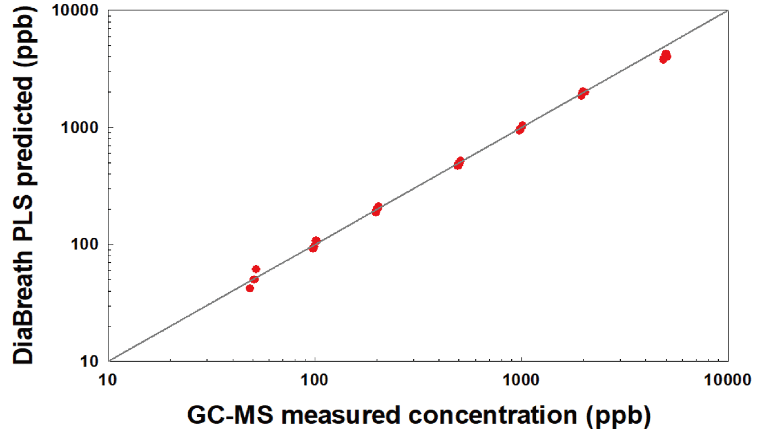
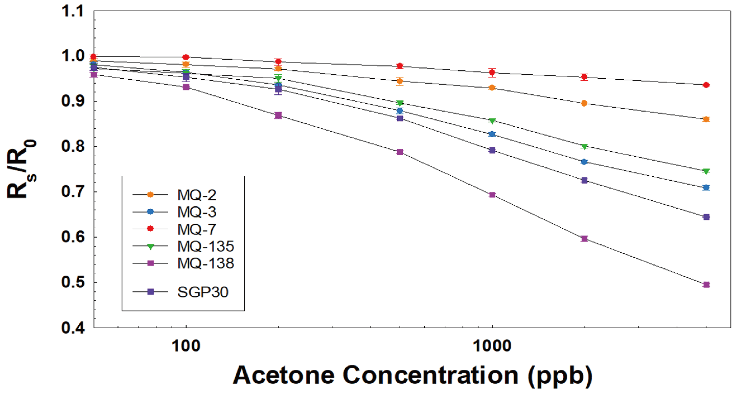
The errors were not the same across the different concentrations. At 50 ppb, the average error was small, but the spread between the three replicates was relatively large (± 9.5 ppb). This is because 50 ppb is close to the detection limit of the sensors, and at this level the sensor signal becomes weak and the readings are not very stable²⁷. At 5 ppm, on the other hand, the error increased to about 19.9%, and the PLS model under-predicted the actual concentration. This under-prediction is related to the nonlinear behavior of the MOX sensors, which can be seen in Figure 6.

Figure 6 shows the R_s/R₀ response of each sensor plotted against the acetone concentration. As the concentration increases, the R_s/R₀ value decreases, but the slope of the curve gradually becomes flatter at higher concentrations. This flattening indicates that the sensors start to saturate as the gas concentration becomes high²⁸. Since the PLS model assumes a linear relationship between the sensor response and the concentration, it cannot fully reflect this saturation effect, and as a result it under-predicts the concentration in the high range.

These results indicate that the MOX sensor array shows different reliability depending on the concentration range. In the range from about 100 ppb to 2 ppm, the array and the PLS model provide concentration estimates that agree well with the GC-MS values. Outside this range, the estimates become less reliable, showing a larger spread at very low concentrations and under-prediction at very high concentrations. However, the acetone level of diabetic breath is usually discussed around 2 ppm, which falls within the range where the array performs reliably, so this limitation has a relatively small effect on the use of the array for diabetes screening.

Breath VOC Screening Model Performance

The four models were trained on the 14,000-sample synthetic breath VOC dataset, and they gave similar results, with test ROC-AUC values all around 0.98 (Table 4). Among them, XGBoost gave the highest test ROC-AUC of 0.9861, so it was chosen as the final model for the breath VOC data.

Model	Accuracy	Precision	Recall	Specificity	F1-score	Train ROC-AUC	Test ROC-AUC
XGBoost	0.9514	0.9585	0.9269	0.9698	0.9424	0.9896	0.9861
Random Forest	0.9542	0.9587	0.9333	0.9698	0.9459	0.9981	0.9862
LightGBM	0.9494	0.9560	0.9245	0.968	0.9400	0.9999	0.9854
Logistic Regression	0.938	0.9397	0.9141	0.956	0.9267	0.9800	0.9802

ROC-AUC was used as the main evaluation metric instead of accuracy. This is because the breath VOC dataset is not perfectly balanced, with about 43% diabetic samples, and a model can get a high accuracy just by leaning toward the majority class. ROC-AUC looks at how well the model separates positive and negative cases regardless of the class ratio, so it is a more reliable metric here. The ROC curve of the final XGBoost model is shown in Figure 7.

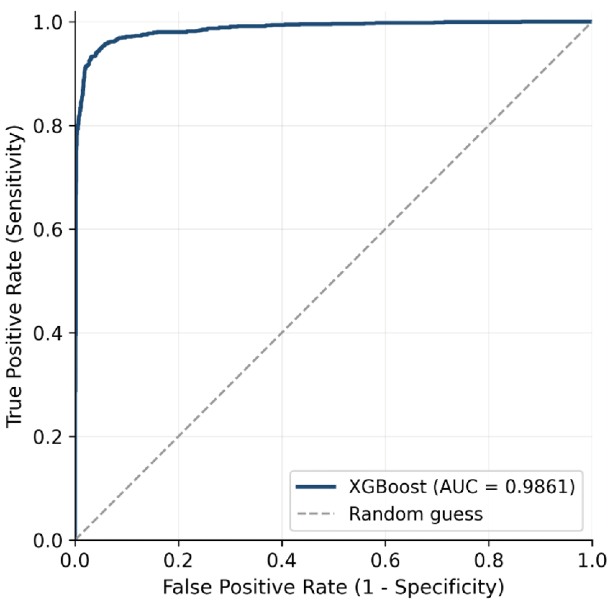
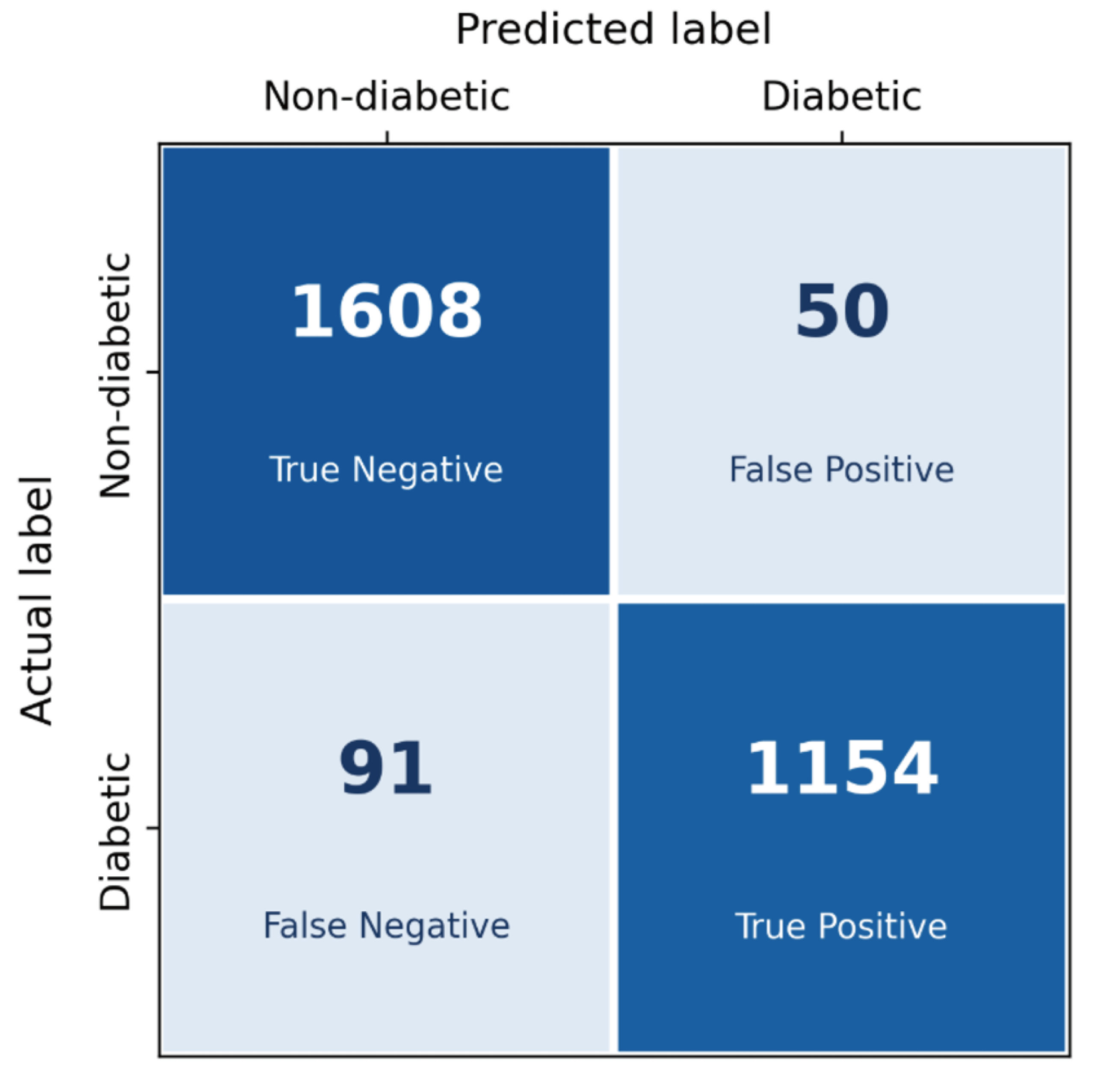
The final XGBoost model reached an accuracy of 0.9514 and a test ROC-AUC of 0.9861. Its train ROC-AUC was 0.9896, which is close to the test value, so the model did not overfit much even on the synthetic data. The recall (sensitivity) was 0.9269 and the specificity was 0.9698, which means the model caught most of the diabetic cases while keeping the false positives low. The confusion matrix of the test set is shown in Figure 8. Out of 1,245 diabetic samples, 1,154 were correctly classified, and out of 1,658 non-diabetic samples, 1,608 were correctly classified.

Hardware and Software Integration

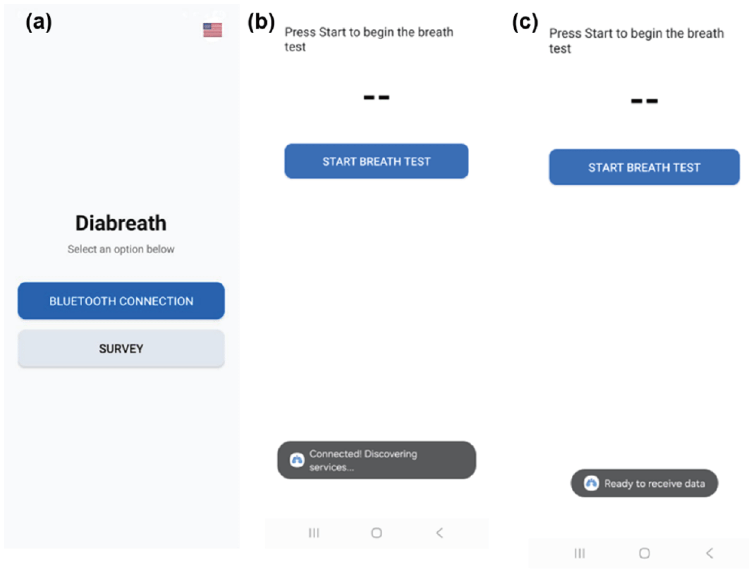
To improve the user-friendliness of the hardware, a smart-device application was created. The application allows user to use DiaBreath without a computer or wired connection, which makes the system more practical for everyday use. When the user opens the application, it first prompts the user to connect to DiaBreath via Bluetooth. Once the connection is established, the user breathes into the hardware, and the sensor array starts collecting R_s/R₀ values from each of the six gas sensors (five MQ-series and one SGP-30). These values are continuously transmitted from the Arduino to the application through the HM-10 Bluetooth module, allowing the data to be received in real time without any cable or serial port (Figure 9).

After the breath data is collected, the application runs the trained XGBoost model on the sensor values and returns a predicted probability of diabetes. The whole process, from the breath measurement to the prediction, runs on the smart device, so no additional hardware is needed besides the device and a smart device. This wireless version improves on the previous version of DiaBreath, where the data was sent to a computer through a cable and serial port.

DiaBreath is intended to be used as a low-cost screening tool, not as a replacement for clinical diagnosis. A positive screening result would still need to be confirmed by a standard clinical test. Combining the breath screening with patient-reported risk factors, such as age and BMI, could give a more complete risk estimate, and this is left as future work.

Discussion

The multivariate analysis results showed that a non-selective MOX sensor array can identify different VOCs and estimate their concentration when the responses of the sensors are combined. Each sensor in the array responds to several gases at the same time, so a single sensor cannot tell one VOC from another. However, when the responses are taken together, they form a multivariate pattern that depends on the type of VOC. From the PCA result, the six VOCs formed separate clusters in the PC1-PC2 space, and the Random Forest classifier showed an accuracy of 0.83. For acetone, the PLS model estimated the concentration with an R² of 0.98 on the UCI dataset within the 50-200 ppb range. Furthermore, to find out whether this also works on the actual device, the DiaBreath measurements were compared with GC-MS. Within the range of 50 ppb to 5 ppm, the predicted values agreed with the GC-MS values with an R² of 0.9900, and near 2 ppm, i.e., the acetone level of diabetic breath, the relative error was only 1.7%. From this, it can be seen that the array carries enough VOC-specific information to estimate the concentration, and that the analytical work moves from the sensor material to the statistical model. However, the agreement was not perfect over the whole range. At 5 ppm, the model showed a lower value than the actual concentration, because the sensors start to saturate at high concentrations and the linear PLS model cannot fully follow this²⁸. Thus, the concentration estimates should be considered reliable within a limited range rather than exact chemical measurements.

For the diabetes screening, the XGBoost model trained on the breath VOC data showed a test ROC-AUC of 0.9861, with a sensitivity of 0.9269 and a specificity of 0.9698. This means the model separated diabetic and non-diabetic samples well on the synthetic data. Previous low-cost e-nose studies showed similar levels of performance. Gudiño-Ochoa et al. reported about 95% accuracy using an MQ-sensor array¹², and a Figaro TGS-array study by Taspinar reported accuracy close to 100% on a larger group¹⁵. Nevertheless, our result was obtained on a synthetic dataset, not on real breath, so it cannot be compared directly with these studies. What this study adds is not a higher accuracy, but a check of whether the sensor array itself can separate and quantify VOCs through multivariate analysis, which most of these studies did not examine.

One of the motivations of this study was to keep the cost low, so the device was built only with inexpensive parts. Table 5 shows the approximate price of each component based on online retail prices. The total comes to under about 60 US dollars, which is much lower than the analytical instruments used for breath analysis. GC-MS, PTR-MS, and SIFT-MS cost from tens of thousands to over a million dollars, so they are hard to use for screening many people⁹. The low cost of DiaBreath comes from the MQ sensors and the Arduino board, i.e., parts that are mass-produced for general use.

Component	Quantity	Approx. price from Amazon (USD)
MQ-series sensors (MQ-2, 3, 7, 135, 138)	5	10
SGP-30 sensor	1	12
Arduino Leonardo	1	22
HM-10 Bluetooth module	1	6
3D-printed PLA shell, breadboard, wires	1 set	8
Total		58

Besides these, several limitations remain. First, the breath VOC dataset was synthetic. It was generated by CTGAN from a smaller set of real breath data, so it is not the same as real breath from real patients. Real breath contains various VOC species, together with humidity and CO₂, so the model performance on real patients may be lower than the value reported in this research. Second, the sensors in DiaBreath are not exactly the same as the ones in the training dataset. And even when the sensor type is the same, the response can change because of calibration, aging, and temperature. This domain shift means the device cannot be assumed to give the same R_s/R₀ distribution as the training data. Third, the device was tested with standard acetone gas under dry nitrogen, without humidity control, so the effect of breath humidity was not included. And the GC-MS validation also showed that the concentration estimates become less reliable at very high concentrations because of the sensor saturation. Fourth, acetone in breath is not unique to diabetes. It also rises during fasting and other metabolic states, so a high acetone reading alone cannot confirm diabetes²⁹.

Furthermore, future work should focus on collecting real breath from diabetic and non-diabetic patients, together with their clinical results such as HbA1c or fasting plasma glucose, so that the model can be trained and tested on real data instead of synthetic data. Patient-reported risk factors such as age and BMI could also be combined with the breath result to give a more complete risk estimate, which was left out of this study. Moreover, to reduce the effect of humidity and temperature, a humidity sensor and a calibration step can be added to the device. With these improvements, it is expected that DiaBreath can be helpful as a low-cost screening tool that supports the standard blood test, especially in the regions where the usual diagnostic methods are hard to reach.

Conclusion

This study showed that a low-cost, non-selective MQ sensor array can identify different VOCs and estimate their concentration when it is combined with multivariate analysis. In the PCA result, the six VOCs were separated into clusters in the PC1-PC2 space, and the Random Forest classifier showed an overall accuracy of 0.83. The PLS regression also showed an R² of 0.98 and an RMSE of 8.77 ppb for acetone in the 50-200 ppb range. And on the actual device, the PLS prediction followed the GC-MS reference with an R² of 0.9900 from 50 ppb to 5 ppm. From these results, it can be seen that the difficult part of the analysis moves from the sensor selectivity to the statistical model, so that inexpensive sensors can be used for VOC quantification within a limited range.

Based on this, the breath VOC model was trained for diabetes screening, and the XGBoost model showed a test ROC-AUC of 0.9861 on the synthetic data. The trained model was embedded into a portable Arduino-based device with six gas sensors and an HM-10 Bluetooth module, which sends the data to a mobile application and runs the breath test without a computer. The component cost of the device was under about 60 US dollars, i.e., much lower than the analytical instruments used for breath analysis.

Several limitations still remain. The breath VOC data used for training was synthetic, not collected from real patients. So the performance on real patients may be lower than the value reported in this research. Furthermore, the sensor array of the device is not exactly the same as the one in the training data. This can cause a domain shift in the R_s/R₀ distribution. The effect of humidity and temperature was also not controlled in this study. Future work should focus on collecting real breath from diabetic and non-diabetic patients together with their clinical results, so that the model can be trained and tested on real data. Age and BMI are patient-reported risk factors, and these could be combined with the breath result for a more complete risk estimate. This was also left as future work. A humidity sensor and a calibration step can be added to the device to reduce the noise from the environment. If these problems are solved, DiaBreath can be helpful as a low-cost screening tool for the A1C blood test, especially in the regions where undiagnosed diabetes mellitus is common.

Acknowledgement

I would like to thank Junhyeok Park for their guidance throughout this research. The author also acknowledges Gudiño-Ochoa et al. for making their synthetic VOC dataset publicly available. This research did not receive any specific grant from funding agencies in the public, commercial, or not-for-profit sectors.

References

1. K. N. C. Duong, C. J. Tan, S. Rattanasiri, A. Thakkinstian, T. Anothaisintawee, N. Chaiyakunapruk. Comparison of diagnostic accuracy for diabetes diagnosis: a systematic review and network meta-analysis. Frontiers in Medicine 10, 1016381 (2023). [↩]
2. K. Ogurtsova, L. Guariguata, N. C. Barengo, P. L. Ruiz, J. W. Sacre, S. Karuranga, H. Sun, E. J. Boyko, D. J. Magliano. IDF diabetes Atlas: Global estimates of undiagnosed diabetes in adults for 2021. Diabetes Research and Clinical Practice 183, 109118 (2022). [↩]
3. S. Saydah, K. Lochner. Socioeconomic status and risk of diabetes-related mortality in the U.S. Public Health Reports 125, 377-388 (2010). [↩] [↩]
4. P. C. Moura, M. Raposo, V. Vassilenko. Breath volatile organic compounds (VOCs) as biomarkers for the diagnosis of pathological conditions: a review. Biomedical Journal 46, 100623 (2023). [↩] [↩]
5. L. Laffel. Ketone bodies: a review of physiology, pathophysiology and application of monitoring to diabetes. Diabetes/Metabolism Research and Reviews 15, 412-426 (1999). [↩]
6. V. Saasa, M. Beukes, Y. Lemmer, B. Mwakikunga. Blood ketone bodies and breath acetone analysis and their correlations in type 2 diabetes mellitus. Diagnostics 9, 224 (2019). [↩] [↩]
7. K. Schwarz, A. Pizzini, B. Arendacká, K. Zerlauth, W. Filipiak, A. Schmid, A. Dzien, S. Neuner, M. Lechleitner, S. Scholl-Bürgi, W. Miekisch, J. Schubert, K. Unterkofler, V. Witkovský, G. Gastl, A. Amann. Breath acetone—aspects of normal physiology related to age and gender as determined in a PTR-MS study. Journal of Breath Research 3, 027003 (2009). [↩]
8. M. Storer, J. Dummer, H. Lunt, J. Scotter, F. McCartin, J. Cook, M. Swanney, D. Kendall, F. Logan, M. Epton. Measurement of breath acetone concentrations by selected ion flow tube mass spectrometry in type 2 diabetes. Journal of Breath Research 5, 046011 (2011). [↩]
9. V. Saasa, T. Malwela, M. Beukes, M. Mokgotho, C.-P. Liu, B. Mwakikunga. Sensing technologies for detection of acetone in human breath for diabetes diagnosis and monitoring. Diagnostics 8, 12 (2018). [↩] [↩]
10. M. Righettoni, A. Tricoli, S. E. Pratsinis. Si:WO3 sensors for highly selective detection of acetone for easy diagnosis of diabetes by breath analysis. Analytical Chemistry 82, 3581-3587 (2010). [↩] [↩]
11. K. Dixit, S. Fardindoost, A. Ravishankara, N. Tasnim, M. Hoorfar. Exhaled breath analysis for diabetes diagnosis and monitoring: relevance, challenges and possibilities. Biosensors 11, 476 (2021). [↩] [↩]
12. A. Gudiño-Ochoa, J. A. García-Rodríguez, J. I. Cuevas-Chávez, R. Ochoa-Ornelas, A. Navarrete-Guzmán, C. Vidrios-Serrano, D. A. Sánchez-Arias. Enhanced diabetes detection and blood glucose prediction using TinyML-integrated E-nose and breath analysis: a novel approach combining synthetic and real-world data. Bioengineering 11, 1065 (2024). [↩] [↩] [↩] [↩]
13. X. Weng, G. Li, Z. Liu, R. Liu, Z. Liu, S. Wang, S. Zhao, X. Ma, Z. Chang. A preliminary screening system for diabetes based on in-car electronic nose. Endocrine Connections 12, e220437 (2023). [↩] [↩]
14. F. A. Bahos, A. Sainz-Vidal, C. Sánchez-Pérez, J. M. Saniger, I. Gràcia, M. M. Saniger-Alba, D. Matatagui. ZIF nanocrystal-based surface acoustic wave (SAW) electronic nose to detect diabetes in human breath. Biosensors 9, 4 (2018). [↩] [↩]
15. Y. S. Taspinar. Machine learning-driven e-nose-based diabetes detection: sensor selection and feature reduction study. Sensors 25, 6607 (2025). [↩] [↩] [↩]
16. F. Tian, L. Zhao, S. Deng. Gas sensor array low-concentration [dataset]. UCI Machine Learning Repository (2023). [↩] [↩]
17. L. Zhao, F. Tian, J. Qian, H. Li, Z. Wu. Feature ensemble learning for sensor array data classification under low-concentration gas. IEEE Transactions on Instrumentation and Measurement 72, 2509112 (2023). [↩] [↩]
18. Z. Wang, C. Wang. Is breath acetone a biomarker of diabetes? A historical review on breath acetone measurements. Journal of Breath Research 7, 037109 (2013). [↩] [↩]
19. C. Wang, L. Yin, L. Zhang, D. Xiang, R. Gao. Metal oxide gas sensors: sensitivity and influencing factors. Sensors 10, 2088-2106 (2010). [↩]
20. Y. Li, X. Wei, Y. Zhou, J. Wang, R. You. Research progress of electronic nose technology in exhaled breath disease analysis. Microsystems & Nanoengineering 9, 129 (2023). [↩]
21. I. Ueta, Y. Saito, M. Hosoe, M. Okamoto, H. Ohkita, S. Shirai, H. Tamura, K. Jinno. Breath acetone analysis with miniaturized sample preparation device: in-needle preconcentration and subsequent determination by gas chromatography-mass spectroscopy. Journal of Chromatography B 877, 2551-2556 (2009). [↩] [↩]
22. T. Chen, C. Guestrin. XGBoost: a scalable tree boosting system. Proceedings of the 22nd ACM SIGKDD International Conference on Knowledge Discovery and Data Mining 785-794 (2016). [↩]
23. G. Ke, Q. Meng, T. Finley, T. Wang, W. Chen, W. Ma, Q. Ye, T.-Y. Liu. LightGBM: a highly efficient gradient boosting decision tree. Advances in Neural Information Processing Systems 30, 3146-3154 (2017). [↩]
24. L. Breiman. Random forests. Machine Learning 45, 5-32 (2001). [↩]
25. T. I. Nasution, R. Asrosa, I. Nainggolan. Application of MQ-138 semiconductor sensor for breath acetone detection. Journal of Physics: Conference Series 1116, 032023 (2018). [↩]
26. P. Paredi, W. Biernacki, G. Invernizzi, S. A. Kharitonov, P. J. Barnes. Exhaled carbon monoxide levels elevated in diabetes and correlated with glucose concentration in blood: a new test for monitoring the disease? Chest 116, 1007-1011 (1999). [↩]
27. W. Shin, S. Hong, Y. Jeong, G. Jung, J. Park, D. Kim, K. Choi, H. Shin, R.-H. Koo, J.-J. Kim, J.-H. Lee. Low-frequency noise in gas sensors: a review. Sensors and Actuators B: Chemical 383, 133551 (2023). [↩]
28. N. Yamazoe, K. Shimanoe. Theory of power laws for semiconductor gas sensors. Sensors and Actuators B: Chemical 128, 566-573 (2008). [↩] [↩]
29. F. Bovey, J. Cros, B. Tuzson, K. Seyssel, P. Schneiter, L. Emmenegger, L. Tappy. Breath acetone as a marker of energy balance: an exploratory study in healthy humans. Nutrition & Diabetes 8, 50 (2018). [↩]